Mean-field description for the architecture of low-energy excitations in glasses
Abstract
In amorphous materials, groups of particles can rearrange locally into a new stable configuration. Such elementary excitations are key as they determine the response to external stresses, as well as to thermal and quantum fluctuations. Yet, understanding what controls their geometry remains a challenge. Here we build a scaling description of the geometry and energy of low-energy excitations in terms of the distance to an instability, as predicted for instance at the dynamical transition in mean field approaches of supercooled liquids. We successfully test our predictions in ultrastable computer glasses, with a gapped and ungapped (regular) spectrum. Overall, our approach explains why excitations become less extended, with a higher energy and displacement scale upon cooling.
I Introduction
If a liquid is cooled rapidly enough to avoid crystallization, its dynamics rapidly slows down until the glass transition where equilibration cannot be achieved: a glass is formed, and the material acts as a solid Ediger et al. 1996. What controls the dynamics in such supercooled liquids is a long-standing question of condensed matter Cavagna 2009; Arceri et al. 2020. Yet, new observations further constrain the descriptions of this phenomenon. The ‘swap’ Monte-Carlo algorithms Briano and Glandt 1984 (in which nearby poly-disperse particles can exchange positions, in addition to their usual translation move) can speed up the dynamics by 15 orders of magnitude or more, and can change the glass transition temperature by up to a factor two Ninarello et al. 2017. Because swap algorithms achieve thermal equilibrium, theories of the glass transition in which thermodynamics governs kinetics Lubchenko and Wolynes 2001; Adam and Gibbs 1965 appear ill suited to explain such a dramatic difference Wyart and Cates 2017 (see Berthier et al. 2019 for an alternative view). Several theoretical works (including real-space Brito et al. 2018, replica Ikeda et al. 2017 and mode-coupling Szamel 2018 approaches) predict that the dynamical transition temperature below which thermal activation becomes the dominant mechanism of relaxation Cavagna 2009 decreases in the presence of swap, plausibly explaining the speed up of this algorithm. However, understanding the dynamics in the vicinity of in finite dimension remains a challenge. By contrast, in the infinite dimensional limit Parisi et al. 2020, mean-field treatments are exact: one finds that for a gap appears in the vibrational spectrum such that there are no vibrational modes with a frequency , whereby grows upon cooling Franz et al. 2015, and that the relaxation time diverges at Maimbourg et al. 2016. For finite , the vibrational spectrum instead presents a pseudo-gap (i.e. the spectrum vanishes as a power-law for small ) consisting of quasi-localized modes (QLMs) Schober et al. 1993. Moreover, thermally activated events or ‘hopping processes’ still occur for , leading to a finite relaxation time. What controls their architecture and energy scale is unclear.
In a parallel development, there has been recently a considerable effort to analyze both QLMs as well as elementary excitations (minimal rearrangements leading to a new metastable state, which form the building blocks of hopping processes) as a function of glass stability Baity-Jesi et al. 2015; Lerner et al. 2016; Mizuno et al. 2017; Lerner and Bouchbinder 2018; Shimada et al. 2018; Scalliet et al. 2019; Wang et al. 2019; Khomenko et al. 2020; Rainone et al. 2020. Numerically, liquids are equilibrated at a parent temperature before being rapidly quenched to , thus obtaining an inherent structure where the Hessian of the energy can be analyzed, and where excitations can be triggered using a short thermal cycle. Strikingly, it is found that the density of excitations is reduced by several decades as decreases Khomenko et al. 2020, and that the characteristic number of particles involved rapidly decreases upon cooling. The former observation is consistent with recent experiments on vapor-deposited glasses Liu et al. 2014; Pérez-Castañeda et al. 2014. Both facts are unexplained.
In this article, (i) we use mean-field and real-space arguments to express the typical scales, namely the length , displacement , number of particles and energy of low-energy excitations, assuming the presence of an underlying gap of magnitude in the vibrational spectrum. We find our predictions to be accurately satisfied in gapped glasses Kapteijns et al. 2019; Ji et al. 2020. (ii) Our analysis implies scaling relations between local properties , that we find to be also satisfied also in regular ultrastable (gapless) glasses. These predictions give a new handle to study the relaxation of glasses. Together with mean field result predicting a growing gap upon cooling, they also explain why low-energy excitations become smaller with a higher energy as the glass stability increases.
The outline of the paper is as follows. In Section II, we provide a scaling description for typical features of local excitations. We then test its predictions first on gapped glasses in Section III, and second on regular ultrastable glasses in Section IV. We conclude in Section V.
II Scaling description for local excitations
We construct scaling relations for local excitations’ typical volume, length, and particle displacement as a function of an underlying . Since the dynamic transition in a mean-field description of liquids corresponds to the point where the Hessian of the energy becomes stable Lubchenko and Wolynes 2007; Franz et al. 2015, we consider a material with a stability control parameter DeGiuli et al. 2014. An instability driven by temperature occurs when approaches , and we thus consider . Infinite dimensional Lubchenko and Wolynes 2007; Franz et al. 2015 calculations as well as effective medium theory DeGiuli et al. 2014 then predict a vanishing minimal eigenvalue of the Hessian that generically depend linearly on , corresponding to a gap frequency above which the spectrum of the Hessian of the energy is a semicircle. In finite dimensions, hopping processes between stable configurations will, however, occur.
To estimate the hopping processes’ spatial extension, we consider two replicas of the system in the glass phase , and denote by their overlap. characterizes the similarity between two configurations at location , and is unity if they are identical 11 1 The overlap between two configurations and can be defined for instance from the square of their Euclidean distance where . A local overlap is then easily obtained by restricting this sum to particles close to position , see also Franz et al. 2012; Guiselin et al. 2020. . In (infinite-dimensional) mean field, the free energy of this coupled system undergoes a saddle-node bifurcation as Franz and Parisi 1998 at which point the overlap is finite; we denote its value . To describe the spatial fluctuations of , we use the following Ginzburg-Landau free energy Biroli et al. 2018; Franz et al. 2011 22 2 In Franz et al. 2011, it is shown that an additional term should enter Eq. 1. This relevant term is equivalent to spatial fluctuations of , and is also present in descriptions of the Random Field Ising Model. As discussed below, the success of our approach suggests that this term is small in our glasses, and will affect physical properties only on length scales beyond those we can reach. , that schematically reads:
| (1) |
At a finite , this free energy has a local minimum at an homogeneous overlap such that , which characterizes the ‘distance’ to the instability. By performing an expansion around , we obtain for overlaps close to the local minimum (only keeping terms that depend on ):
| (2) |
The overlap displays thermal fluctuations, whose length scale and correlation volume can be deduced from the correlation function . For the quadratic free energy of Eq. 1, when with the correlation length, this classical computation (see Appendix A)) gives:
| (3) |
A similar length scale was predicted to affect the dynamics in mode-coupling theory Franz and Parisi 2000; Biroli et al. 2006 and was observed to characterize the linear response near an instability Lerner et al. 2014. Eq. 3 also leads to a characteristic volume in which fluctuations are correlated. The typical volume of an excitation can be related to the correlation length by the spatial integration (where ), which is independent of dimension. Such a quadratic relation between volume and length is already known to hold near jamming Yan et al. 2016; Shimada et al. 2018. We thus have . In , it implies dimensionally that , where is the characteristic particle size. In what follows we make the natural assumption that low-energy elementary excitations do occur on the characteristic volume and length scale of spontaneous fluctuations, such that their number of particles and their length .
To obtain the characteristic displacement and energy scale of such local excitations, we perform an expansion of a symmetric double well (for an asymmetric double well, both the energy barrier and difference generically scale as the result we obtain Ji et al. 2020). Here is the norm of the displacement field of the excitation, that satisfies where is the typical particle displacement. By analyzing the extrema of , one readily obtains that the energy barrier between the two minima is 33 3 In Ji et al. 2020, was assumed to be a constant, leading to the incorrect relation . and the distance between the local minima follows , implying that .
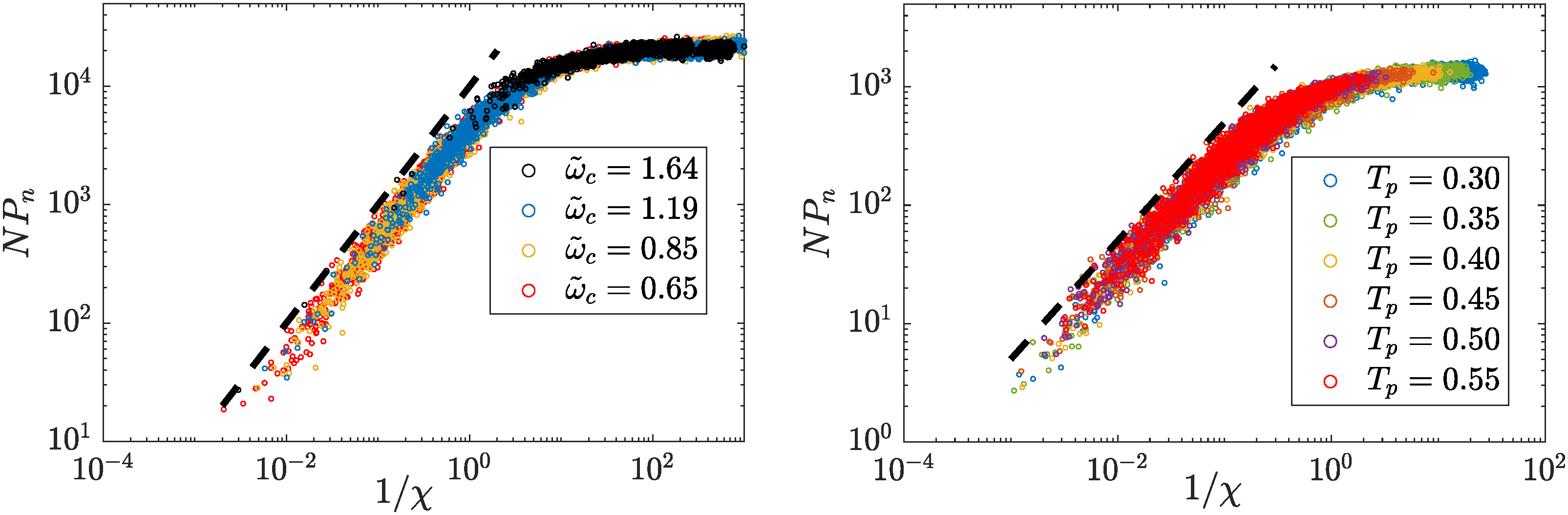
Ultimately, the term stems from the quartic non-linearity in the inter-particle interaction potential (which we assume to be short ranged). We denote its characteristic magnitude , a microscopic quantity, which is thus finite even as . Writing that the total quartic term is a sum of the microscopic ones, leads to , implying that . This scaling relation is confirmed empirically for QLMs in Appendix C. We thus obtain and . In summary, we get the following scaling description (disregarding constant prefactors):
| (4) |
Thus, we predict that close to an instability (e.g. ), hopping processes are extended with small characteristic displacement and energy scales. Away from an instability, on the contrary, they become localized with large displacements and energy.
III Gapped glasses
We first test Eq. 4 in three-dimensional gapped glasses, obtained with ‘breathing’ particles Brito et al. 2018; Kapteijns et al. 2019. We use the protocol and parameters of Ji et al. 2020 reviewed in Appendix B. In a nutshell, we perform molecular dynamics (MD) simulations in which the radius of all particles is an additional degree of freedom, whose stiffness controls the particle polydispersity. A long run at finite temperature is followed by an instantaneous quench using the “FIRE” algorithm to zero temperature. We then freeze the particle radii and measure the vibrational spectrum, which presents a gap of magnitude that strongly depends on .
Next, we study elementary excitations using thermally activated rearrangements. They are obtained by heating our samples with standard (non-breathing) MD to a temperature for a duration , followed by an instantaneous quench using again the “FIRE” algorithm to zero temperature. In practice, and are chosen so as to trigger one rearrangement per sample in average. In practice we observe up to 4 rearrangements per sample in practice, which we then separate in individual ones using an algorithm developed in Ji et al. 2020. A displacement field , which is a vector of dimension , is associated to each excitation. We focus on elementary excitations that go to higher energy states. In doing so, we eliminate events where one double well is very asymmetric and lies close to a saddle-node bifurcation (and would then present a tiny activation barrier not captured by our scaling assuming a symmetric well). These events can also be suppressed if the quench is not instantaneous, as we use below for regular glasses.
For each , we obtain of the order of excitations. We consider the median of the following observables: (i) The number of particles involved in a rearrangement , where is the participation ratio of . (ii) The particle characteristic displacement where . (iii) The length , defined from the second moment of the position of the particles involved in the rearrangement. Namely, where , and is the relative position of particle with respect to the center of the rearrangement. (iv) The energy difference before and after the rearrangement . We compare this last quantity to another estimate of the characteristic energy, obtained in Ji et al. 2020. In particular, after thermal cycling, the density of quasi-localized modes no longer presents a gap. Rather it presents a pseudo-gap for small . From it, we extract a characteristic energy scale by fitting by an Arrhenius behavior.
Our results are presented in Fig. 1 (left column) (see Appendix D for the whole distributions): the vanishing scale of particle displacement is tested in panel (a), and in (b). It is found to be slightly smaller but comparable to the previously reported quantity (open markers) Ji et al. 2020. is tested in panel (c), and in (d). Overall, we find a good agreement between our scaling predictions and measurements.
IV Regular ultrastable glasses
In regular glasses, the density of QLMs does not display a gap Baity-Jesi et al. 2015; Lerner et al. 2016; Mizuno et al. 2017 even before reheating. Indeed, at any finite temperature a gap must necessarily fill up in finite dimensions, because some excitations transition to their high energy state. If the latter is barely stable, a low-frequency quasi-localized mode appears (see illustration in Appendix E). This effect does not affect the scalings of excitations (which are unchanged), but it leads to the emergence of a pseudo-gap Ji et al. 2020 that makes the characteristic frequency hard to extract.
Moreover, in finite dimension due to the spatial heterogeneity of the material, the distance to an elastic instability must vary spatially. This effect is a relevant perturbation: exponents entering Eq. 3 should depart from their mean-field value Biroli et al. 2018; Franz et al. 2011. Yet, if these structural fluctuations are small, they will affect exponents only at large length scales inaccessible in glasses 44 4 The marginality condition is not observed even when quenching from high temperatures, leading to a finite length scale DeGiuli et al. 2014. , and mean-field exponents will be observed. As shown above, it appears to be the case in our very homogeneous gapped glass. Yet, it may not be so in ‘normally‘ prepared ultra-stable glasses.
To study this question, we focus on the local scaling relationships that follow from Eq. 4, which can readily be tested. Configurations equilibrated by swap at different parent temperature are taken from Rainone et al. 2020 who used the specific liquid model of Lerner 2019, that we then instantaneously quench from to , followed by a small cooling rate to zero temperature. This preparation protocol is used so as to minimize the number of modes that are close to an instability. Thus it limits the number of excitations that go to a lower energy state upon temperature cycling, and allows us to more easily sample statistics on the excitations increasing energy.
For each , we again obtain of the order of excitations of these inherent structures through temperature cycles at a low and a short time , from which , , and are then extracted. As shown in Fig. 1, right column, we again find a very good agreement with our predictions: the geometrical description of localized excitations that follows from Eq. 4 appears to hold also in regular glasses. We checked that the scaling predictions also hold well at other two higher reheating temperatures (see Appendix F). Thus a simple mean-field approach already captures the geometry and energy of excitations quite satisfyingly 55 5 When the displacements becomes of order of the particle size, we found for the gapped glass that a small fraction of excitations are strings Ji et al. 2020. As we will report elsewhere, it is also true for regular glasses. Although strings are presumably not accurately described by mean-field argument, their fraction is small: removing them from the statistics does not change our observations. .
Our second claim is that the increased stability upon cooling predicted by mean-field methods (corresponding to a growing characteristic frequency as decreases), together with our scaling relations Eq. 4, imply that in regular glasses local excitations must then become less extended and involve fewer particles –precisely as has been observed in the literature Lerner et al. 2016; Mizuno et al. 2017; Lerner and Bouchbinder 2018; Scalliet et al. 2019; Wang et al. 2019; Khomenko et al. 2020; Rainone et al. 2020, and confirmed in Fig. 1(g,h). We further predict that the characteristic energy of excitations and the displacement should (rapidly) increase upon cooling (i.e. decreasing ) as confirmed in Fig. 1(e,f).
Note that a (crude) estimate of some effective can be obtained by comparing the displacement magnitude of the lowest-energy excitations in our samples, to those of gapped samples, i.e. comparing Figs. 1(a) and (e), which corresponds to a rapidly growing characteristic frequency upon cooling (see Appendix G for details).
V Conclusion
We have developed a scaling description for the architecture of local excitations in glasses, expressed in terms of the distance to an elastic instability where their characteristic length diverges. In gapped glasses obtained with breathing particles, this distance is embodied in the magnitude of the gap . This description appears to provide guidance in regular glasses as well, where a characteristic frequency is more challenging to identify from the vibrational spectrum Ji et al. 2020.
Using the mean-field result that the gap grows upon cooling together with our arguments explains why excitations become less extended upon cooling, and leads to two other confirmed predictions. First, excitations have larger displacements in stable glasses. Second, we predict a rapidly growing low energy scale for local excitations, corresponding to two decades in the temperature range probed as apparent in Fig. 1(f). The density of two-level systems should be diminished by this growing energy, as observed numerically Khomenko et al. 2020; Khomenko et al. 2021, since it implies a larger tunneling barrier that will eventually become hard to overcome by quantum fluctuations on experimental time scales Ji et al. 2020.
Note that our mean-field arguments appear to yield appropriate exponents in three-dimensional simulations, at least in the limited range accessible in glasses Berthier and Biroli 2011. This situation is reminiscent of the jamming literature DeGiuli et al. 2014; Parisi et al. 2020, and suggests that structural disorder in glasses induces limited heterogeneities in their elastic properties. It would be interesting to design a Ginzburg criterion, in the spirit of Franz et al. 2012, to estimate beyond which length scale finite dimensional effects could be detectable.
Another interesting question concerns the differences between the geometry of QLMs and excitations Khomenko et al. 2021. In particular, the length scale below which continuum elasticity breaks down when a force dipole is exerted Lerner et al. 2014, reported to characterize the core of QLMs Shimada et al. 2018; Rainone et al. 2020, also decreases under cooling Rainone et al. 2020. In Appendix H, we observe that indeed decouples from the excitations length scale in our most stable glasses (gapped or regular).
Looking forward, the scaling description of low-energy elementary excitations in glasses may give a new handle to describe hopping processes in glasses, going beyond simple ‘elastic’ models proposed in the past Dyre 2006. A positive item is their predicted rapidly growing energy scale under cooling, reminiscent of the fragility of liquids. Yet, a description of all elementary excitations (not only the low-energy ones studied here) is ultimately needed to make progress on that long-standing question.
Acknowledgements.
We thank M. Müller and M. Popović for discussions at the earlier stages of this work, and G. Biroli, J.P. Bouchaud, S. Franz and D. Reichman for discussions. We thank the authors of Rainone et al. 2020 for providing us with equilibrated swap configurations and discussions. T.G. acknowledges support from the Swiss National Science Foundation (SNSF) by the SNSF Ambizione Grant PZ00P2_185843, E.A. by the SNSF Ambizione Grant PZ00P2_173962. We thank the Simons Foundation Grant (#454953 Matthieu Wyart) and the SNSF under Grant No. 200021-165509 for support.Appendix A Derivation of correlation function
For pedagogical completeness, here we rederive the correlation function of the overlap , which is a standard result from the Ginzburg-Landau theory developed in critical phenomena. Note that we denote the distance explicitly, while in the main text we use translational invariance to render the notation shorter.
Let us define . The two-point correlation function is defined as an average over all possible overlap configurations, with a weight given by the free-energy . It thus reads:
| (5) |
Note that is a functional integral over all possible overlap configurations, and the last line is obtained by integrating by parts.
Because this path integral has been put in a quadratic form, this simply amounts to computing a Gaussian integral where the operator is the functional inverse of the correlator . This literally means that and must satisfy the relation
| (6) |
This differential equation can be easily solved in Fourier space, for instance. In direct space, when , we reach the Eq. (3) in the main text:
with .
Appendix B Parameters
| Gapped glasses | ||||||||||
| separation | ||||||||||
| 1.64 | yes | |||||||||
| yes | ||||||||||
| yes | ||||||||||
| yes | ||||||||||
| Regular glasses | ||||||||||
| separation | ||||||||||
| no | ||||||||||
| no | ||||||||||
| no | ||||||||||
| no | ||||||||||
| no | ||||||||||
| no | ||||||||||
We list all parameters beyond those listed in Ji et al. 2020; Lerner 2019; Rainone et al. 2020. For gapped glasses we use ensembles comprising samples at particles in three dimensions for four different gap frequencies (, see below for the definition of ), prepared by Ji et al. 2020. For regular glasses we use ensembles comprising configurations at particles in three dimensions for six different parent temperatures , prepared by Rainone et al. 2020. The relevant parameters are listed in Table 1, where, in addition to the parameters described in the text:
- •
, the typical inter-particle distance, is defined as the peak in the particle-particle correlation function.
- •
is the total number of excitations triggered using temperature cycling; is the number of excitations going to higher energy minima (‘positive’ excitations).
- •
is the Debye frequency, with the particle number density and the volume; and are the transverse and longitudinal velocity, related to the shear modulus and bulk modulus ; is the particle mass (taken equal for all particles).
- •
is the summation of pair interaction energy divided by .
Note that , , , and are obtained as average values of sample-to-sample fluctuating quantities.
The units in Table 1 are as follows. Length () is in units of , the initial diameter of small particles in gapped glasses, and the diameter of smallest particles in regular glasses (particles sizes are inverse power law distributed, and is the smallest diameter i.e. the lower bound of the diameter distribution). Energy () is in units of , the prefactor of the inter-particle interaction potential. Temperature ( and ) is in units of , where we set Boltzmann’s constant to . Time (, , ) is in units of , where is the particle mass (equal for all particles). Bulk modulus and shear modulus are in units of .
Note, furthermore, that: (i) In preparing regular glasses, a protocol is adopted where we instantaneously quench to , and then slowly quench rate at a rate so that the fraction of ‘positive’ excitation is not low (see Table 1). We checked that if the glasses are instead prepared by instantaneous quench (like we do for the ‘breathing’ particles), not more than of excitations are ‘positive’ excitations at the highest we consider, which is inefficient to obtain good statistics. (ii) Since less than 10% of samples rearrange in regular glasses, we assume that each rearrangement is an elementary excitation, and we do not apply our separation algorithm Ji et al. 2020. (iii) For the ‘breathing particles’ the pressure is fixed to a constant value. This is why is different at different , and we adopt the notation , with the volume of the individual samples. In regular glasses, instead, the volume is fixed to a constant value.
Appendix C Quartic term for quasi-localized modes
Here we show that the participation ratio of quasi-localized modes is proportional to the inverse of the coefficient of quartic term along quasi-localized modes, both in gapped glasses and in regular glasses. In particular, where is the eigenmode component on the th particle. where the is the fourth order (spatial) derivative of the total interaction potential energy, it is a rank four tensor of size . For details see Gartner and Lerner 2016; Ji et al. 2020. The scatter plots in Fig. 2, show that at low the scaling is consistent with . We use 25 samples at gapped glasses and 100 samples at in regular glasses to calculate and , and these samples are also used in Appendix H.
Appendix D Distributions for hopping processes
Fig. 3 shows the distributions of the bare quantities , of the energy difference , of the length , and of thermally-activated rearrangements, i.e. ‘hopping processes’. The medians are shown using a vertical line, defining , , , and . Data are taken with the conditioning on excitations going to higher energy state: both in gapped glasses (first row) and regular glasses (second) row. Distributions are peaked around a maximum, except for the energy distribution whose distribution is maximum in zero (corresponding to symmetric double wells).
Appendix E Filling up the gap
Fig. 4 shows that, in finite dimension, the gap in the vibrational spectrum is filled up by thermally activating excitations. In particular, we expect that upon reheating with a small temperature, the vibrational spectrum is filled up with modes with excitations from a ‘reservoir’ of excitations at frequencies Ji et al. 2020. This process corresponds to excitations moving from a lower energy minima with a characteristic frequency to a higher one with characteristic frequency . Ultimately, this effect leads to a pseudo-gap at . Yet, the excitations responsible for populating the gap have a characteristic frequency in their lower-energy state, and their architecture and energy must follow our predictions for a gap of magnitude .
Appendix F Different reheating temperatures (regular glasses)
Fig. 5 investigates the scaling predictions at three temperature in regular glasses. The results found are overall robust toward the change of . We can still discern some systematic effects: excitations have a larger energy, present larger displacements and involve more particles as increases.
Appendix G Crude estimate of in regular glass
In this section, we estimate in regular glasses. We suppose in gapped glasses and regular glasses varies with in the same way. Since we know both and in gapped glasses, we fit the data by to extract and . We employ them to get an estimate of at the lowest energy excitations (lowest at each ). The results, in Fig. 6, increases with decreasing , as we expect.
Appendix H Measurement of
To extract the typical global length , we perturb the glasses with a local dipole force and look at the correlation function which is defined in as Lerner et al. 2014; Rainone et al. 2020. is defined as the length where rescaling collapses the data, see Fig. 7. Note that for this global measurement we use a bigger system ( samples at ; whereby we checked that these collapse the rescaled at as well, except for a small difference at our smallest gap) at each in gapped glasses, and samples at at each in regular glasses to extract .
In Fig. 8, we show that decouples from the excitation length scale in stable (i.e. gapped and regular) glasses, at large .
References
- Ediger et al. [1996] M. Ediger, C. Angell, and S. Nagel, The journal of physical chemistry 100, 13200 (1996).
- Cavagna [2009] A. Cavagna, Phys. Rep. 476, 51 (2009).
- Arceri et al. [2020] F. Arceri, F. Landes, L. Berthier, and G. Biroli, arXiv preprint: 2006.09725 (2020), 10.48550/arXiv.2006.09725.
- Briano and Glandt [1984] J. Briano and E. Glandt, J. Chem. Phys. 80, 3336 (1984).
- Ninarello et al. [2017] A. Ninarello, L. Berthier, and D. Coslovich, Phys. Rev. X 7, 021039 (2017).
- Lubchenko and Wolynes [2001] V. Lubchenko and P. Wolynes, Phys. Rev. Lett. 87, 195901 (2001).
- Adam and Gibbs [1965] G. Adam and J. Gibbs, J. Chem. Phys. 43, 139 (1965).
- Wyart and Cates [2017] M. Wyart and M. Cates, Phys. Rev. Lett. 119, 195501 (2017).
- Berthier et al. [2019] L. Berthier, G. Biroli, J.-P. Bouchaud, and G. Tarjus, J. Chem. Phys. 150, 094501 (2019).
- Brito et al. [2018] C. Brito, E. Lerner, and M. Wyart, Phys. Rev. X 8, 031050 (2018).
- Ikeda et al. [2017] H. Ikeda, F. Zamponi, and A. Ikeda, J. Chem. Phys. 147, 234506 (2017).
- Szamel [2018] G. Szamel, Phys. Rev. E 98, 050601(R) (2018).
- Parisi et al. [2020] G. Parisi, P. Urbani, and F. Zamponi, Cambridge University Press, Theory of Simple Glasses: Exact Solutions in Infinite Dimensions (2020).
- Franz et al. [2015] S. Franz, G. Parisi, P. Urbani, and F. Zamponi, Proc. Natl. Acad. Sci. 112, 14539 (2015).
- Maimbourg et al. [2016] T. Maimbourg, J. Kurchan, and F. Zamponi, Phys. Rev. Lett. 116, 015902 (2016).
- Schober et al. [1993] H. Schober, C. Oligschleger, and B. Laird, J. Non. Cryst. Solids 156-158, 965 (1993).
- Baity-Jesi et al. [2015] M. Baity-Jesi, V. Martín-Mayor, G. Parisi, and S. Perez-Gaviro, Phys. Rev. Lett. 115, 267205 (2015).
- Lerner et al. [2016] E. Lerner, G. Düring, and E. Bouchbinder, Phys. Rev. Lett. 117, 035501 (2016).
- Mizuno et al. [2017] H. Mizuno, H. Shiba, and A. Ikeda, Proc. Natl. Acad. Sci. 114, E9767 (2017).
- Lerner and Bouchbinder [2018] E. Lerner and E. Bouchbinder, J. Chem. Phys. 148, 214502 (2018).
- Shimada et al. [2018] M. Shimada, H. Mizuno, M. Wyart, and A. Ikeda, Phys. Rev. E 98, 060901(R) (2018).
- Scalliet et al. [2019] C. Scalliet, L. Berthier, and F. Zamponi, Nat. Commun. 10, 5102 (2019).
- Wang et al. [2019] L. Wang, A. Ninarello, P. Guan, L. Berthier, G. Szamel, and E. Flenner, Nat. Commun. 10, 26 (2019).
- Khomenko et al. [2020] D. Khomenko, C. Scalliet, L. Berthier, D. Reichman, and F. Zamponi, Phys. Rev. Lett. 124, 225901 (2020).
- Rainone et al. [2020] C. Rainone, E. Bouchbinder, and E. Lerner, Proc. Natl. Acad. Sci. 117, 5228 (2020).
- Liu et al. [2014] X. Liu, D. Queen, T. Metcalf, J. Karel, and F. Hellman, Phys. Rev. Lett. 113, 025503 (2014).
- Pérez-Castañeda et al. [2014] T. Pérez-Castañeda, C. Rodríguez-Tinoco, J. Rodríguez-Viejo, and M. Ramos, Proc. Natl. Acad. Sci. 111, 11275 (2014).
- Kapteijns et al. [2019] G. Kapteijns, W. Ji, C. Brito, M. Wyart, and E. Lerner, Phys. Rev. E 99, 012106 (2019).
- Ji et al. [2020] W. Ji, T. de Geus, M. Popović, E. Agoritsas, and M. Wyart, Phys. Rev. E 102, 062110 (2020).
- Lubchenko and Wolynes [2007] V. Lubchenko and P. Wolynes, Ann. Phys. Chem. 58, 235 (2007).
- DeGiuli et al. [2014] E. DeGiuli, A. Laversanne-Finot, G. Düring, E. Lerner, and M. Wyart, Soft Matter 10, 5628 (2014).
- Franz et al. [2012] S. Franz, H. Jacquin, G. Parisi, P. Urbani, and F. Zamponi, Proc. Natl. Acad. Sci. 109, 18725 (2012).
- Guiselin et al. [2020] B. Guiselin, G. Tarjus, and L. Berthier, J. Chem. Phys. 153, 224502 (2020).
- Franz and Parisi [1998] S. Franz and G. Parisi, Phys. A 261, 317 (1998).
- Biroli et al. [2018] G. Biroli, C. Cammarota, G. Tarjus, and M. Tarzia, Phys. Rev. B 98, 174206 (2018).
- Franz et al. [2011] S. Franz, G. Parisi, F. Ricci-Tersenghi, and T. Rizzo, Eur. Phys. J. E 34, 102 (2011).
- Franz and Parisi [2000] S. Franz and G. Parisi, J. Phys. Condens. Matter 12, 6335 (2000).
- Biroli et al. [2006] G. Biroli, J.-P. Bouchaud, K. Miyazaki, and D. Reichman, Phys. Rev. Lett. 97, 195701 (2006).
- Lerner et al. [2014] E. Lerner, E. DeGiuli, G. Düring, and M. Wyart, Soft Matter 10, 5085 (2014).
- Yan et al. [2016] L. Yan, E. DeGiuli, and M. Wyart, Europhys. Lett. 114, 26003 (2016).
- Lerner [2019] E. Lerner, J. Non-Cryst. Solids 522, 119570 (2019).
- Khomenko et al. [2021] D. Khomenko, D. Reichman, and F. Zamponi, Phys. Rev. Materials 5, 055602 (2021).
- Berthier and Biroli [2011] L. Berthier and G. Biroli, Rev. Mod. Phys. 83, 587 (2011).
- Dyre [2006] J. Dyre, Rev. Mod. Phys. 78, 953 (2006).
- Gartner and Lerner [2016] L. Gartner and E. Lerner, SciPost Phys. 1, 016 (2016).