Unifying Gradient Estimators for Meta-Reinforcement Learning via Off-Policy Evaluation
Abstract
Model-agnostic meta-reinforcement learning requires estimating the Hessian matrix of value functions. This is challenging from an implementation perspective, as repeatedly differentiating policy gradient estimates may lead to biased Hessian estimates. In this work, we provide a unifying framework for estimating higher-order derivatives of value functions, based on off-policy evaluation. Our framework interprets a number of prior approaches as special cases and elucidates the bias and variance trade-off of Hessian estimates. This framework also opens the door to a new family of estimates, which can be easily implemented with auto-differentiation libraries, and lead to performance gains in practice. We open source the code to reproduce our results11 1 https://github.com/robintyh1/neurips2021-meta-gradient-offpolicy-evaluation.
1 Introduction
Recent years have witnessed the success of reinforcement learning (RL) in challenging domains such as game playing [1], board games [2], and robotics control [3]. However, despite such breakthroughs, state-of-the-art RL algorithms are still plagued by sample inefficiency, as training agents requires orders of magnitude more samples than humans would experience to reach similar levels of performance [1, 2]. One hypothesis on the source of such inefficiencies is that standard RL algorithms are not good at leveraging prior knowledge, which implies that whenever presented with a new task, the algorithms must learn from scratch. On the contrary, humans are much better at transferring prior skills to new scenarios, an innate ability arguably obtained through evolution over thousand of years.
Meta-reinforcement learning (meta-RL) formalizes the learning and transfer of prior knowledge in RL [4]. The high-level idea is to have an RL agent that interacts with a distribution of environments at meta-training time. The objective is that at meta-testing time, when the agent interacts with previously unseen environments, it can learn much faster than meta-training time. Here, faster learning is measured by the number of new samples needed to achieve a good level of performance. If an agent can achieve good performance at meta-testing time, it embodies the ability to transfer knowledge from prior experiences at meta-training time. meta-RL algorithms can be constructed in many ways, such as those based on recurrent memory [5, 6], gradient-based adaptations [4], learning loss functions [7, 8, 9], probabilistic inference of context variables [10, 11, 12], online adaptation of hyper-parameters within a single lifetime [13, 14] and so on. Some of these formulations have mathematical connections; see e.g. [15] for an in-depth discussion.
We focus on gradient-based adaptations [4], where the agent carries out policy gradient updates [16] at both meta-training and meta-testing time. Conceptually, since meta-RL seeks to optimize the way in which the agent adapts itself in face of new environments, it needs to differentiate through the policy gradient update itself. This effectively reduces the meta-RL problem into estimations of Hessian matrices of value functions.
Challenges for computing Hessian matrix of value functions.
To calculate Hessian matrices (or unbiased estimates thereof) for supervised learning objectives, it suffices to differentiate through gradient estimates, which can be easily implemented with auto-differentiation packages [17, 18, 19]. However, it is not the case for value functions in RL. Intuitively, this is because value functions are defined via expectations with respect to distributions that themselves depend on the policy parameters of interest, whereas in supervised learning the expectations are defined with respect to a fixed data distribution. As a result, implementations that do not take this into account may lead to estimates [4] whose bias is not properly characterized and might have a negative impact on downstream applications [20].
Motivated by this observation, a number of prior works suggest implementation alternatives that lead to unbiased Hessian estimates [21], with potential variance reduction [22, 23, 20]; or biased estimates with small variance [24]. However, different algorithms in this space are motivated and derived in seemingly unrelated ways: for example, [21, 22, 23] derive code-level implementations within the general context of stochastic computation graphs [25]. On the other hand, [24] derives the estimates by explicitly analyzing certain terms with potentially high variance, which naturally produces bias in the final estimate. Due to apparently distinct ways of deriving estimates, it is not immediately clear how all such methods are related, and whether there could be other alternatives.
| Off-policy evaluation estimates | Step-wise IS [26] | Doubly-robust [27] | TayPO- [28, 29] | TayPO- [29] |
| Prior work | DiCE [21] | Loaded DiCE [22, 23] | LVC [24] | Second-order (this work) |
Central contribution.
We present a unified framework for estimating higher-order derivatives of value functions, based on the concept of off-policy evaluation. The main insights are summarized in Table 1, where most aforementioned prior work can be interpreted as special cases of our framework. Our framework has a few advantages: (1) it conceptually unifies a few seemingly unrelated prior methods; (2) it elucidates the bias and variance trade-off of the estimates; (3) it naturally produces new methods based on Taylor expansions of value functions [29].
After a brief background introduction on meta-RL in Section 2, we will discuss the above aspects in detail in Section 3. From an implementation perspective, we will show in Section 4.1 that both the general framework and the new method can be conveniently implemented in auto-differentiation libraries [30, 19], making it amenable in a practical setup. Finally in Section 5, we validate important claims based on this framework with experimental insights.
2 Background
We begin with the notation and background on RL and meta-RL.
2.1 Task-based reinforcement learning
Consider a Markov decision process (MDP) with state space and action space . At time , the agent takes action in state , receives a reward and transitions to a next state . Without loss of generality, we assume a single starting state . Here, we assume the reward to be a deterministic function of state-action pair and the task variable . The task variable is resampled for every episode. For example, is the sensory space of a running robot, is the control, is the episodic target direction in which to run and is the speed in direction . A policy specifies a distribution over actions at each state. For convenience, we define the value function and Q-function . Without loss of generality, we assume the policy to be smoothly parameterized as with parameter . We further assume that the MDPs terminate within a finite horizon of under any policy.
2.2 Gradient-based meta-reinforcement learning
The motivation of meta-RL is to identify a policy such that given a task , after updating the parameter from to with a parameter update computed under rewards , the resulting policy performs well. Formally, define as a parameter update to , for example, one policy gradient ascent step. Model-agnostic meta-learning (MAML) [4] formulates meta-RL as optimizing the value function at the updated policy where is the updated policy. The optimization is with respect to the initial policy parameter . The aim is to find such that it entails fast learning (or adaptation) to the environment, through the inner loop update operator , that leads to high-performing updated policy . Consider the following problem,
| (1) |
We can decompose the meta-gradient into two terms based on the chain rule,
| (2) |
where is a matrix, and is the vanilla policy gradient evaluated at the updated parameter [31]. A straightforward way to optimizing Eqn (1) is to carry out the outer loop update with learning rate .
Policy gradient update.
Following MAML [4], we focus on policy gradient update where for a fixed step size . The matrix is the Hessian of the value function with respect to policy parameters; henceforth, we define .
Estimating meta-gradients.
Practical algorithms construct stochastic estimates of the meta-gradients using a finite number of samples. In Eqn (2), we decompose the meta-gradients into the multiplication of a Hessian matrix with a policy gradient vector. Given a fixed task variable , a common practice of prior work is to construct the gradient estimate as the product of the Hessian estimate and the policy gradient estimate ; see, e.g., [4, 32, 33, 24, 21, 22, 23, 20]. See Algorithm 1 for the full pseudocode for estimating meta-gradients by sampling multiple tasks. Since there is a large literature on constructing accurate estimates to policy gradient (e.g., actor-critic algorithms use baselines for variance reduction [34]), the main challenge consists in estimating the Hessian matrix accurately.
Bias of common plug-in estimators.
Common practices in meta-RL algorithms rely on the premise that if both Hessian and policy gradient estimates are unbiased, then the meta-gradient estimate is unbiased too.
Unfortunately, this is not true. This is because the two estimates are in general correlated when the sample size is finite, leading to the bias of the overall estimate. We provide further discussions in Appendix A. For the rest of the paper, we follow practices of prior work and focus on the properties of Hessian estimates, leaving a more proper treatment of this bias to future work.
3 Deriving Hessian estimates with off-policy evaluation
Since the meta-gradient estimates are computed by averaging over task variables , in the following, we focus on Hessian estimates at a single state and task variable with a fixed . In this section, we also drop the dependency of the value function on , such that, e.g., and .
3.1 Off-policy evaluation: maintaining higher-order dependencies on parameters
We assume access to data generated under a behavior policy . Off-policy evaluation [26] consists in building estimators using the behavior data such that for a range of target policies . Note that the estimate is a random variable depending on , it is also a function of . The approximation implies that is indicative of how the value function depends on , and hence maintains the higher-order dependencies on . Throughout, we assume for all .
Example: step-wise importance sampling (IS) estimate.
As a concrete example, consider the unbiased step-wise IS estimate where . Since the value function is in general a highly non-linear function of (see discussions in [35]) we see that retains such dependencies via the sum of product of IS ratios.
3.2 Warming up: deriving unbiased estimates with variance reduction
We start with a general result based on the intuition above: given an estimate to , we can directly use the th-order derivative as an estimate to . We introduce two assumptions: (A.1) is th-order differentiable w.r.t. almost surely. (A.2) for some constant for the order of interest. These assumptions are fairly mild; see further details in Appendix C. The following result applies to general unbiased off-policy evaluation estimates.
Proposition 3.1.
Assume (A.1) and (A.2) are satisfied. Further assume we have an estimator which is unbiased () for all where is some open set that contains . Under some additional mild conditions, the th-order derivative of the estimate are unbiased estimates to the th-order derivative of the value function for .
Doubly-robust estimates.
As a special case, we describe the doubly-robust (DR) off-policy evaluation estimator [36, 27, 37]. Assume we have access to a state-action dependent critic , and we use the notation . The DR estimate is defined recursively as follows,
| (3) |
The DR estimate is unbiased for all and subsumes the step-wise IS estimate as a special case when . If the critic is properly chosen, e.g., , it can lead to significant variance reduction compared to . By directly differentiating the estimate , we derive estimators for higher-order derivatives of the value function; the result for the gradient in Proposition 3.2 was shown in [38].
Proposition 3.2.
Define and let be the sampled temporal difference error at time . Note that and . The estimates of higher-order derivatives can be deduced recursively, and in particular for ,
| (4) | ||||
| (5) |
Bias and variance of Hessian estimates.
Proposition 3.1 implies that and are both unbiased. To analyze the variance, we start with : note that when on-policy [16], recovers a form of gradient estimates similar to actor-critic policy gradient with action-dependent baselines [39, 40, 41]; when is only state dependent, recovers the common policy gradient estimate with state-dependent baselines [34]. As such, the estimates are computed with potential variance reduction due to the critic. Previously, [38] started with the DR estimate and derived a more general result for the on-policy first-order case. For the Hessian estimate, we expect a similar effect of variance reduction as shown in experiments.
Recovering prior work on estimates to higher-order derivatives.
When applied to meta-RL, DiCE [21] and its follow-up variants [22, 42] can be seen as special cases of with different choices of the critic when evaluated on-policy . See Table 1 for the correspondence between prior work and their equivalent formulations under the framework of off-policy evaluation. We will discuss detailed pseudocode in Section 4.1. See also Appendix F for more details.
3.3 Trading-off bias and variance with Taylor expansions
Starting from unbiased off-policy evaluation estimates , we can directly construct unbiased estimates to higher-order derivatives by differentiating the original estimate to obtain . However, unbiased estimates can have large variance. Though it is possible to reduce variance through the critic, as we will show experimentally, this is not enough to counter the high variance due to products of IS ratios. This leads us to consider trading off bias with variance [43].
Since we postulate that the products of IS ratios lead to high variance, we might seek to control the number of IS ratios in the estimate. We briefly introduce Taylor expansion policy optimization (TayPO) [29], a natural framework to control for the number of IS ratios in the value estimate.
Taylor expansions of value functions.
Consider the value function as a function of . Using the idea of Taylor expansions, we can express as a sum of polynomials of . We start by defining the th-order increment as , which does not contain any IS ratio (zeroth order); and for ,
| (6) |
Intuitively, the th-order increment only contains product of IS ratios. Equation (6) also yields a natural sample-based estimate , which we will discuss later. The th-order Taylor expansion is defined as the partial sum of increments . Since consists of products of up to IS ratios, it is effectively the th-order Taylor expansion of the value function. The properties are summarized as follows.
Proposition 3.3.
(Adapted from Theorem 2 of [29].) Define . Let be a constant and . Then the following holds for all ,
| (7) |
If , then .
Sample-based estimates to Taylor expansions of value functions.
As shown in Equation (6), is an unbiased estimate to . We can naturally define the sample-based estimate to the th-order Taylor expansion, called the TayPO- estimate,
| (8) |
The expression of contains terms if the trajectory is of length . Please refer to Appendix E for further details on computing the estimates in linear time with sub-sampling. Note that is a sample-based estimate whose bias against the value function is controlled by the residual term which decays exponentially when and are close. Similar to how we derived the unbiased estimate , we can differentiate through the TayPO- value estimate to produce estimates to higher-order derivatives .
Bias and variance of Hessian estimates.
TayPO- trades-off bias and variance with choices of . To understand the variance, note that TayPO- limits the number multiplicative IS ratios to be . Though it is difficult to compute the variance, we argue that the variance generally increases with as the number of IS ratios increase [26, 27, 44]. We characterize the bias of TayPO- as follows.
Proposition 3.4.
Assume (A.1) and (A.2) hold. Also assume . For any tensor , define . The th-order TayPO objective produces the following bias in estimating high-order derivatives,
| (9) |
Hence the upper bound for the bias decreases as increases. Importantly, when on-policy , the th-order TayPO objective preserves up to th-order derivatives for any ,
| (10) |
Though IS ratios evaluate to when on-policy, they maintain the parameter dependencies in differentiations. As such, higher-order expansions contains products of IS ratios of higher orders, and maintains the high-order dependencies on parameters more accurately. There is a clear trade-off between bias and variance mediated by . When increases, the higher-order derivatives are maintained more accurately in expectation, leading to less bias. However, the variance increases too.
Recovering prior work as special cases.
Recently, [24] proposed a low variance curvature (LVC) Hessian estimate. This estimate is equivalent to the TayPO- estimate with . As also noted by [24], their objective function bears similarities to first-order policy search algorithms [28, 45, 46], which have in fact been interpreted as first-order special cases of with [29]. Importantly, based on Proposition 3.4, the LVC estimate only maintains the first-order dependency perfectly but introduces bias when approximating the Hessian, even when on-policy.
Limitations.
Though the above framework interprets a large number of prior methods as special cases, it has some limitations. For example, the derivation of Hessian estimates based on the DR estimate (Proposition 3.2) involves estimates of the value function . In practice, when near on-policy , one might replace the DR estimate by other value function estimate, such as plain cumulative sum of returns or TD(), [22, 23] in Eqn (4). As such, the practical implementation might not strictly adhere to the conceptual framework. In addition, TMAML [20] is not incorporated as part of this framework: we show in Appendix B that the control variate introduced by TMAML in fact biases the overall estimate.
4 From Hessian estimates to meta-gradient estimates
A practical desiteratum for meta-gradient estimates is that it can be implemented in a scalable way using auto-differentiation frameworks [30, 19]. Below, we discuss how this can be achieved.
4.1 Auto-differentiating off-policy evaluation estimates for Hessian estimates
In practice, we seek Hessian estimates that could be implemented with the help of an established framework, such as auto-differentiation libraries [30, 19]. Now we discuss how to conveniently implement ideas discussed in the previous section.
Auto-differentiating the estimates.
We can abstract the off-policy evaluation as a function that takes in some data and parameter , and outputs an estimate for . In particular, includes the trajectories and is input via the policy . As an example, Algorithm 2 shows that for the doubly-robust estimator, the dependency of the estimator on is built through the recursive computation by . In fact, if we implement Algorithm 2 with an auto-differentiation framework (for example, Tensorflow or PyTorch [17, 18, 19]), the higher-order dependency of on is maintained through the computation graph. We can compute the Hessian estimate by directly differentiating through the function output . In Appendix F we show how the estimates could be conveniently implemented, as in many deep RL agents (see, e.g., [44, 5, 47, 48]). We also show concrete ways to compute estimates with TayPO- based on [29].
4.2 Practical implementations of meta-gradient estimates
In Equation (2), we write the meta-gradient estimate as a product between an Hessian estimate and a policy gradient. In practice, the meta-gradient estimate is computed via Hessian-vector products to avoid explicitly computing the Hessian estimate of size . As such, the meta-gradient estimate could be computed by auto-differentiating through a scalar objective. See Appendix F for details.
Bias and variance of meta-gradient estimates.
Intuitively, the bias and variance of the Hessian estimates translate into bias and variance of the downstream meta-gradient estimates. Prior work has showed that low variance of meta-gradient estimates lead to faster convergence [49, 50]. However, it is not clear how the bias (such as bias introduced by the Hessian estimates, or the bias due to correlated estimates) theoretically impacts the convergence. We will study empirically the effect of bias and variance in experiments, and leave further theoretical study to future work.
5 Experiments
We now carry out several empirical studies to complement the framework developed above. In Section 5.1, we use a tabular example to investigate the bias and variance trade-offs of various estimates, to assess the validity of our theoretical insights. We choose a tabular example because it is straightforward to compute exact higher-order derivatives of value functions and make comparison. In Section 5.2.1 and Section 5.2.2, we apply the new second-order estimate in high-dimensional meta-RL experiments, to assess the potential performance gains in a more practical setup. Though we can compute TayPO- order estimates for general , we focus on in experiments. Below, we also address TayPO- and TayPO- estimates as the first and second-order estimates respectively.
5.1 Investigating the bias and variance trade-off of different estimates
We study the bias and variance trade-off of various estimates using a tabular exmaple. We consider random MDPs with . The transition matrix of the MDPs are sampled from a Dirichlet distribution. See Appendix G for further details. The policy is parameterized as . The behavior policy is uniform and is initialized so that where for some deterministic policy and parameter . The hyper-parameter measures the off-policyness. In this example, there is no task variable. As performance metrics, we measure the component-wise correlation between the true derivatives (computed via an oracle) where is a fixed starting state, and its estimates , as commonly used in prior work [21, 22, 23]. The estimates are averaged across samples. We study the effect of different choices of the off-policy estimate , as a function of off-policyness and sample size . We report results with over seeds.


Effect of off-policyness.
In Figure 1(a) and (b), we let and show the performance as a function of . When increases (more off-policy), the accuracy measures of most estimates decrease. This is because off-policyness generally increases both bias and variance (large IS ratios ). At this level of sample size, the performance of the second-order estimate degrades more slowly than other estimates, making it the dominating estimate across all values of . We also include truncated DR estimate using as a baseline inspired by V-trace [44, 47]. The truncation is motivated by controlling the variance of the overall estimate. However, the estimate is heavily biased and does not perform well unless . See Appendix F for more.
Consider the case when and the setup is on-policy. When estimating the policy gradient, almost all estimates converge to the optimal level of accuracy, except for the step-wise IS estimate, where the variance still renders the performance sub-optimal. However, when estimating the Hessian matrix, the first-order estimate converges to a lower accuracy than both second-order estimate and DR estimate. This validates our theoretical analysis, as both the second-order estimate and DR estimate are unbiased when on-policy.
Effect of sample size.
Figure 1(c) shows the accuracy measures as a function of sample size when fixing . Note that since sample sizes directly influence the variance, the results show the variance properties of different estimates. When is small, the first-order estimate dominates due to smaller variance; however, when increases, the first-order estimate is surpassed by the second-order estimate, due to higher bias. For more results and ablation on high-dimensional environments, see Appendix G.
5.2 High-dimensional meta-RL problems
Next, we study the practical gains entailed by the second-order estimate in high-dimensional meta-RL problems. We first introduce a few important algorithmic baselines, and how the second-order estimate is incorporated into a meta-RL algorithm.
Baseline algorithms.
All baseline algorithms use plain stochastic gradient ascent as the inner loop optimizer: where is a sampled goal and is a sample-based estimate of policy gradients averaged over trajectories. Different algorithms differ in how the inner loop loss is implemented, such that auto-differentiation produces different Hessian estimates: these include TRPO-DiCE [21, 22, 23], TRPO-MAML [4], TRPO-FMAML [4], TRPO-EMAML [32, 33]. Please refer to Appendix G for further details. Note despite the name, TRPO-DiCE baseline uses DR estimate to estimate Hessians. We implement the second-order estimate using the proximal meta policy search (PROMP) [24] as the base algorithm. By default, PROMP uses the first-order estimate. Our new algorithm is named PROMP-TayPO-.
5.2.1 Continuous control in 2D environments
Environment.
We consider a simple -D navigation task introduced in [24]. The state is the coordinate of a ball placed inside a room, the action is the direction in which to push the ball. The goal is an one-hot encoding of which corner of the room contains positive rewards. With adaptation steps, the agent should ideally navigate to the desired corner indicated by .
Training performance.
In Figure 1(d), we show the performance curves of various baseline algorithms. Though MAML and EMAML learns quickly during the initial phase of training, they ultimately become unstable. TRPO-DiCE generally underperforms other methods potentially due to bias. On the other hand, FMAML and PROMP both reduce variance at the cost of bias, but they both achieve a slightly lower level of performance compared to PROMP-TayPO-. Overall, PROMP-TAyPO- achieves much more stable training curves compared to others, potentially owing to the better bias and variance trade-off in the Hessian estimates.
5.2.2 Large scale locomotion experiments
Environments.
We consider the set of meta-RL tasks based on simulated locomotion in MuJoCo [51]. Across these tasks, the states consist of robotic sensory inputs, the actions are torque controls applied to the robots. The task is defined per environment: for example, in random goal environment, is a random -d goal location that the robot should aim to reach.
Experiment setup.
We adapt the open source code base by [24] and adopt exactly the same experimental setup as [24]. At each iteration, the agent samples task variables. For each task, the agent carries out adaptation computed based on trajectories sampled from the environment, each of length . See Appendix G for further details on the architecture and other hyper-parameters. We report averaged results with over seeds.


Results.
The training performance of different algorithmic baselines are shown in Figure 2. Comparing TRPO-DiCE, TRPO-MAML and PROMP: we see that the results are compatible with those reported in [24], where PROMP outperforms TRPO-MAML, while TRPO-DiCE generally performs the worst potentially due to high variance in the gradient estimates. As a side observation, TRPO-FMAML generally underperforms TRPO-MAML, which implies the necessity of carrying out approximations to the Hessian matrix beyond the identity matrix. PROMP-TayPO- slightly outperforms PROMP in a few occasions, where the new algorithm achieves slightly faster learning speed and sometimes higher final performance. However, overall, we see that the empirical gains are marginal. This implies that under the default setup of these meta-RL experiments, the variance might be a major factor in gradient estimates, and the first-order estimate is near optimal compared to other estimates. See Appendix G for additional experiments.
6 Conclusion
We have unified a number of important prior work on meta-gradient estimations for model-agnostic meta-RL. Our analysis entails the derivations of prior methods based on the unifying framework of differentiating through off-policy evaluation estimates. This framework provides a principled way to reason about the bias and variance in the higher-order derivative estimates of value functions, and opens the door to a new family of estimates based on novel off-policy evaluation estimates. As an important example, we have theoretically and empirically studied the properties of the family of TayPO-based estimates. It is worth noting that this framework further suggests any future advances in off-policy evaluation could be conveniently imported into potential improvements in meta-gradient estimates. As future work, we hope to see the applications of such principled estimates in broader meta-RL applications.
Acknowledgement.
The authors thank David Abel for reviewing an early draft of this work and providing very useful feedback. Yunhao and Tadashi are thankful for the Scientific Computation and Data Analysis section at the Okinawa Institute of Science and Technology (OIST), which maintains a cluster we used for many of our experiments.
References
- [1] Volodymyr Mnih, Koray Kavukcuoglu, David Silver, Alex Graves, Ioannis Antonoglou, Daan Wierstra, and Martin Riedmiller. Playing atari with deep reinforcement learning. arXiv preprint arXiv:1312.5602, 2013.
- [2] David Silver, Aja Huang, Chris J Maddison, Arthur Guez, Laurent Sifre, George Van Den Driessche, Julian Schrittwieser, Ioannis Antonoglou, Veda Panneershelvam, Marc Lanctot, et al. Mastering the game of go with deep neural networks and tree search. nature, 529(7587):484–489, 2016.
- [3] Sergey Levine, Chelsea Finn, Trevor Darrell, and Pieter Abbeel. End-to-end training of deep visuomotor policies. The Journal of Machine Learning Research, 17(1):1334–1373, 2016.
- [4] Chelsea Finn, Pieter Abbeel, and Sergey Levine. Model-agnostic meta-learning for fast adaptation of deep networks. In International Conference on Machine Learning, pages 1126–1135. PMLR, 2017.
- [5] Ziyu Wang, Tom Schaul, Matteo Hessel, Hado Van Hasselt, Marc Lanctot, and Nando De Freitas. Dueling network architectures for deep reinforcement learning. arXiv preprint arXiv:1511.06581, 2015.
- [6] Yan Duan, John Schulman, Xi Chen, Peter L Bartlett, Ilya Sutskever, and Pieter Abbeel. Rl2: Fast reinforcement learning via slow reinforcement learning. arXiv preprint arXiv:1611.02779, 2016.
- [7] Rein Houthooft, Richard Y Chen, Phillip Isola, Bradly C Stadie, Filip Wolski, Jonathan Ho, and Pieter Abbeel. Evolved policy gradients. arXiv preprint arXiv:1802.04821, 2018.
- [8] Junhyuk Oh, Matteo Hessel, Wojciech M Czarnecki, Zhongwen Xu, Hado van Hasselt, Satinder Singh, and David Silver. Discovering reinforcement learning algorithms. arXiv preprint arXiv:2007.08794, 2020.
- [9] Zhongwen Xu, Hado van Hasselt, Matteo Hessel, Junhyuk Oh, Satinder Singh, and David Silver. Meta-gradient reinforcement learning with an objective discovered online. arXiv preprint arXiv:2007.08433, 2020.
- [10] Kate Rakelly, Aurick Zhou, Chelsea Finn, Sergey Levine, and Deirdre Quillen. Efficient off-policy meta-reinforcement learning via probabilistic context variables. In International conference on machine learning, pages 5331–5340. PMLR, 2019.
- [11] Luisa Zintgraf, Kyriacos Shiarlis, Maximilian Igl, Sebastian Schulze, Yarin Gal, Katja Hofmann, and Shimon Whiteson. Varibad: A very good method for bayes-adaptive deep rl via meta-learning. arXiv preprint arXiv:1910.08348, 2019.
- [12] Rasool Fakoor, Pratik Chaudhari, Stefano Soatto, and Alexander J Smola. Meta-q-learning. arXiv preprint arXiv:1910.00125, 2019.
- [13] Zhongwen Xu, Hado P van Hasselt, and David Silver. Meta-gradient reinforcement learning. In Advances in neural information processing systems, pages 2396–2407, 2018.
- [14] Tom Zahavy, Zhongwen Xu, Vivek Veeriah, Matteo Hessel, Junhyuk Oh, Hado van Hasselt, David Silver, and Satinder Singh. A self-tuning actor-critic algorithm. arXiv preprint arXiv:2002.12928, 2020.
- [15] Pedro A Ortega, Jane X Wang, Mark Rowland, Tim Genewein, Zeb Kurth-Nelson, Razvan Pascanu, Nicolas Heess, Joel Veness, Alex Pritzel, Pablo Sprechmann, et al. Meta-learning of sequential strategies. arXiv preprint arXiv:1905.03030, 2019.
- [16] Richard S Sutton, David A McAllester, Satinder P Singh, and Yishay Mansour. Policy gradient methods for reinforcement learning with function approximation. In Advances in neural information processing systems, pages 1057–1063, 2000.
- [17] Kavosh Asadi and Michael L Littman. An alternative softmax operator for reinforcement learning. In International Conference on Machine Learning, pages 243–252, 2017.
- [18] James Bradbury, Roy Frostig, Peter Hawkins, Matthew James Johnson, Chris Leary, Dougal Maclaurin, George Necula, Adam Paszke, Jake VanderPlas, Skye Wanderman-Milne, and Qiao Zhang. JAX: composable transformations of Python+NumPy programs, 2018.
- [19] Adam Paszke, Sam Gross, Soumith Chintala, Gregory Chanan, Edward Yang, Zachary DeVito, Zeming Lin, Alban Desmaison, Luca Antiga, and Adam Lerer. Automatic differentiation in pytorch. 2017.
- [20] Hao Liu, Richard Socher, and Caiming Xiong. Taming maml: Efficient unbiased meta-reinforcement learning. In International Conference on Machine Learning, pages 4061–4071. PMLR, 2019.
- [21] Jakob Foerster, Gregory Farquhar, Maruan Al-Shedivat, Tim Rocktäschel, Eric Xing, and Shimon Whiteson. Dice: The infinitely differentiable monte carlo estimator. In International Conference on Machine Learning, pages 1529–1538. PMLR, 2018.
- [22] Gregory Farquhar, Shimon Whiteson, and Jakob Foerster. Loaded dice: Trading off bias and variance in any-order score function gradient estimators for reinforcement learning. 2019.
- [23] Jingkai Mao, Jakob Foerster, Tim Rocktäschel, Maruan Al-Shedivat, Gregory Farquhar, and Shimon Whiteson. A baseline for any order gradient estimation in stochastic computation graphs. In International Conference on Machine Learning, pages 4343–4351. PMLR, 2019.
- [24] Jonas Rothfuss, Dennis Lee, Ignasi Clavera, Tamim Asfour, and Pieter Abbeel. Promp: Proximal meta-policy search. arXiv preprint arXiv:1810.06784, 2018.
- [25] John Schulman, Nicolas Heess, Theophane Weber, and Pieter Abbeel. Gradient estimation using stochastic computation graphs. In Advances in Neural Information Processing Systems, pages 3528–3536, 2015.
- [26] Doina Precup, Richard S Sutton, and Sanjoy Dasgupta. Off-policy temporal-difference learning with function approximation. In ICML, pages 417–424, 2001.
- [27] Nan Jiang and Lihong Li. Doubly robust off-policy value evaluation for reinforcement learning. In International Conference on Machine Learning, pages 652–661. PMLR, 2016.
- [28] Sham Kakade and John Langford. Approximately optimal approximate reinforcement learning. In ICML, volume 2, pages 267–274, 2002.
- [29] Yunhao Tang, Michal Valko, and Rémi Munos. Taylor expansion policy optimization. arXiv preprint arXiv:2003.06259, 2020.
- [30] Martín Abadi, Paul Barham, Jianmin Chen, Zhifeng Chen, Andy Davis, Jeffrey Dean, Matthieu Devin, Sanjay Ghemawat, Geoffrey Irving, Michael Isard, et al. Tensorflow: A system for large-scale machine learning. In 12th USENIX symposium on operating systems design and implementation (OSDI 16), pages 265–283, 2016.
- [31] Richard S Sutton and Andrew G Barto. Reinforcement learning: An introduction, volume 1. MIT press Cambridge, 1998.
- [32] Maruan Al-Shedivat, Trapit Bansal, Yuri Burda, Ilya Sutskever, Igor Mordatch, and Pieter Abbeel. Continuous adaptation via meta-learning in nonstationary and competitive environments. arXiv preprint arXiv:1710.03641, 2017.
- [33] Bradly C Stadie, Ge Yang, Rein Houthooft, Xi Chen, Yan Duan, Yuhuai Wu, Pieter Abbeel, and Ilya Sutskever. Some considerations on learning to explore via meta-reinforcement learning. arXiv preprint arXiv:1803.01118, 2018.
- [34] Vijay R Konda and John N Tsitsiklis. Actor-critic algorithms. In Advances in neural information processing systems, pages 1008–1014. Citeseer, 2000.
- [35] Alekh Agarwal, Sham M Kakade, Jason D Lee, and Gaurav Mahajan. Optimality and approximation with policy gradient methods in markov decision processes. In Conference on Learning Theory, pages 64–66. PMLR, 2020.
- [36] Miroslav Dudík, Dumitru Erhan, John Langford, Lihong Li, et al. Doubly robust policy evaluation and optimization. Statistical Science, 29(4):485–511, 2014.
- [37] Philip Thomas and Emma Brunskill. Data-efficient off-policy policy evaluation for reinforcement learning. In International Conference on Machine Learning, pages 2139–2148. PMLR, 2016.
- [38] Jiawei Huang and Nan Jiang. From importance sampling to doubly robust policy gradient. In International Conference on Machine Learning, pages 4434–4443. PMLR, 2020.
- [39] Hao Liu, Yihao Feng, Yi Mao, Dengyong Zhou, Jian Peng, and Qiang Liu. Action-depedent control variates for policy optimization via stein’s identity. arXiv preprint arXiv:1710.11198, 2017.
- [40] Cathy Wu, Aravind Rajeswaran, Yan Duan, Vikash Kumar, Alexandre M Bayen, Sham Kakade, Igor Mordatch, and Pieter Abbeel. Variance reduction for policy gradient with action-dependent factorized baselines. arXiv preprint arXiv:1803.07246, 2018.
- [41] George Tucker, Surya Bhupatiraju, Shixiang Gu, Richard Turner, Zoubin Ghahramani, and Sergey Levine. The mirage of action-dependent baselines in reinforcement learning. In International conference on machine learning, pages 5015–5024. PMLR, 2018.
- [42] Horia Mania, Aurelia Guy, and Benjamin Recht. Simple random search provides a competitive approach to reinforcement learning. arXiv preprint arXiv:1803.07055, 2018.
- [43] Mark Rowland, Will Dabney, and Rémi Munos. Adaptive trade-offs in off-policy learning. arXiv preprint arXiv:1910.07478, 2019.
- [44] Rémi Munos, Tom Stepleton, Anna Harutyunyan, and Marc Bellemare. Safe and efficient off-policy reinforcement learning. In Advances in Neural Information Processing Systems, pages 1054–1062, 2016.
- [45] John Schulman, Sergey Levine, Pieter Abbeel, Michael Jordan, and Philipp Moritz. Trust region policy optimization. In International Conference on Machine Learning, pages 1889–1897, 2015.
- [46] John Schulman, Filip Wolski, Prafulla Dhariwal, Alec Radford, and Oleg Klimov. Proximal policy optimization algorithms. arXiv preprint arXiv:1707.06347, 2017.
- [47] Lasse Espeholt, Hubert Soyer, Remi Munos, Karen Simonyan, Volodymir Mnih, Tom Ward, Yotam Doron, Vlad Firoiu, Tim Harley, Iain Dunning, et al. Impala: Scalable distributed deep-rl with importance weighted actor-learner architectures. arXiv preprint arXiv:1802.01561, 2018.
- [48] Steven Kapturowski, Georg Ostrovski, John Quan, Remi Munos, and Will Dabney. Recurrent experience replay in distributed reinforcement learning. 2018.
- [49] Alireza Fallah, Aryan Mokhtari, and Asuman Ozdaglar. On the convergence theory of gradient-based model-agnostic meta-learning algorithms. In International Conference on Artificial Intelligence and Statistics, pages 1082–1092. PMLR, 2020.
- [50] Kaiyi Ji, Junjie Yang, and Yingbin Liang. Multi-step model-agnostic meta-learning: Convergence and improved algorithms. arXiv preprint arXiv:2002.07836, 2020.
- [51] Emanuel Todorov, Tom Erez, and Yuval Tassa. Mujoco: A physics engine for model-based control. In Intelligent Robots and Systems (IROS), 2012 IEEE/RSJ International Conference on, pages 5026–5033. IEEE, 2012.
- [52] Diederik P Kingma and Max Welling. Auto-encoding variational bayes. arXiv preprint arXiv:1312.6114, 2013.
Appendix A Bias with practical estimations of meta-gradients
Recall the MAML objective defined in Eqn (1). The adapted parameter is computed with the expected policy gradient update . This makes it difficult to construct fully unbiased estimates to the MAML gradient. We use a following example to show the intuitions.
Consider a scalar objective with input . If it is possible to construct unbiased estimate to , i.e., with such that . It is difficult to construct unbiased estimates to because unless is linear.
Conceptually, we can think of the argument here as the updated parameter resulting from expected updates . It is convenient to construct unbiased estimate of this parameter because it is convenient to build unbiased estimate to the policy gradient . However, in our case, to compute the meta RL gradients, we need to evaluate the policy gradient at : , which is usually an highly non-linear function of . Using the notation of the above scalar objective example, we can construct a vector valued function: . Though it is straightforward to construct unbiased estimates to with sampled trajectories, it is not easy to estimate in an unbiased way, as a direct plug in would be biased.
Appendix B Proof on the bias of TMAML
Below, we adopt the trajectory-based notation of TMAML [20]. Let , where the operation removes the dependency of on parameter . In other words, . It is worth noting that the stop gradient notations are equivalent to the derivation that defines with a fixed behavior policy , and later sets , as done in the main paper. TMAML [20] proposed the following baseline objective in the undiscounted finite horizon case with horizon ,
where is a baseline function that depends on state . The major claim from TMAML [20] is that , which implies that adding to the original DICE objective [21] might lead to variance reduction because it serves as a control variate term. However, below we show
The proof proceeds in deriving the explicit expression for . We derive the same expression as that in the Appendix C of the original paper [20], i.e.,
| (11) |
Following the proof of [20], it is then straightforward to show that
| (12) |
However, note the difference between Eqn (11) and Eqn (12) lies in the summation instead of . Accounting for this difference, we have
which in general does not evaluate to zero. In fact, the bias of is clear if we take the special case . In this case, it is more straightforward to derive
As a result, we showed that TMAML [20] might achieve variance reduction by introducing baselines to the Hessian estimates of DiCE [21], but at the cost of bias.
Appendix C Further discussions on the assumptions
In this section, we examine if the assumptions (A.1) and (A.2) are realistic.
Both assumptions depend on particular functional form of the estimates . In general, we might assume that the estimates do not explicitly depend on . Instead, they depend on via . This involves a two-stage parameterization: and . The two assumptions (A.1) and (A.2) can be realized by imposing constraints on these two parameterizations, as well as the off-policyness of relative to , as discussed below.
Off-policyness.
Parameterization .
We seek parameterizations where are bounded. This can be achieved by bounding and . If we consider a tabular representation with softmax parameterization . Under this parameterization, we can show are bounded for all and all .
Parameterization .
We want this parameterization to be sufficiently smooth. In the examples we consider, TayPO- clearly satisfies this assumption because it is a polynomial in . For DR, this assumption is satisfied when the MDP terminates within a finite horizon of , such that the estimator contains polynomials of with order at most .
Appendix D Proof of results in the main paper
See 3.1
Proof.
The two assumptions along with the unbiasedness of the estimates, allow us to exchange th-order derivatives and the expectation, and hence leading to the unbiasedness of the derivate estimates. The proof is similar to the exchange techniques used in [38] to show the unbiasedness of the first-order derivatives of DR estimates.
We proceed the argument with induction. Assume we have
for some . To define the -th order derivative, we differentiate further through the -th order derivative. Consider some particular component of the -th order derivative, obtained by taking the derivative with respect to variable . We now denote this component of the -th order derivative as evaluated at . Let denote the -th order derivative (a tensor) evaluated at . Also define as the one-hot vector such as its -th component is one. By definition,
we also denote the unbiased estimate to as . The new estimate is
Now we seek to establish that . Note that this is equivalent to showing
Note that with the RHS, we can use the definition along with unbiasedness of the -th order derivatives
Combining the new RHS into a single expectation, (A.1) entails the application of the mean value theorem,
for some . Due to (A.2), we can use dominated convergence theorem to exchange the limit and the expectation,
This proves the case for -th order derivative. The base case holds for and we have the assumptions hold for all . This concludes the proof of the theorem.
∎
See 3.2
Proof.
Starting from the definition of the DR estimate in Eqn (3), which we recall here
Note that both sides of the equations are functions of . Since the DR estimate holds for all (assuming has larger support than ), and both sides are differentiable functions of . We can differentiate both sides of the equation with respect to , to yield its th-order derivatives. This produces the gradient estimates and the Hessian estimates accordingly, both in recursive forms.
The first term.
This term produces a single term .
The second term.
Note a few useful facts: , . This produces
The third term.
Finally, the third term produces
Combining all three terms produces the recursive form of the DR Hessian estimates.
∎
See 3.4
Proof.
We can express the residual of the derivatives as
Above, the first equality comes from the unbiasedness of the estimates as well as the exchangability between derivatives and expectations, following similar arguments as those in Proposition 3.1. The second equality comes from the Taylor expansion equality in Proposition 3.3. By the assumption that the MDP terminates within an horizon of , we deduce that the summation contains at most terms and it is valid to exchange derivatives and the summation. Eqn (9) is hence proved by applying the triangle inequality.
When on-policy, we plug in . Since , this implies that after differentiating for a total of times, each term contains at least terms of for some . Since , this means for all indices within the summation. Hence we have zeros on the RHS and this shows Eqn (10). ∎
Appendix E Further details on sampled-based TayPO- estimates
Please refer to the TayPO [29] paper for further theoretical discussions. By definition, the th-order increment is
Assume the trajectory is of finite length (or we can use the effective horizon . The naive Monte-Carlo estimate consists of terms. Since we usually care about , computing such a term exactly might still be tractable, as is shown later in Appendix F. We show in Algorithm 4 how to compute the estimates with complexity .
However, in some applications, we might seek to construct the estimates with better time complexity. The high-level idea is to achieve this through sub-sampling. Define , where is the probability measure induced by and the MDP. We can rewrite the above into the following
where the sequence of states are sampled as and . Note that the above procedure could be achieved by first generating a full trajectory under , and then sub-sampling random times along the trajectory. As such, the estimate takes linear time to compute, at the cost of potentially larger variance.
Appendix F High-level code for implementations of Hessian estimates and meta-gradients
Below, we introduce a few important details on how to convert off-policy evaluation estimates into Hessian estimates, with the help of auto-diff.
F.1 Implementing Hessian estimates with off-policy evaluation subroutines
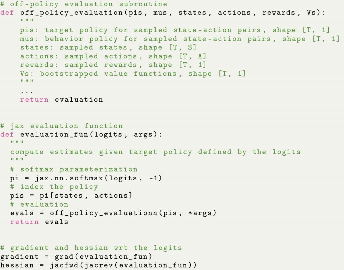
In Figure 3, we show a high-level JAX implementation of estimating Hessians using off-policy evaluiation subroutines. The pseudocode assumes access to some well-established off-policy evaluation functions, as are commonly implemented in off-policy RL algorithms such as ACER [5], Retrace [44], IMPALA [47], R2D2 [48] and so on. The function needs to be written in auto-differentiation libraries, such that after the computations, value function estimates’ parameter dependencies are naturally maintained. Then this pipeline could be directly implemented as part of a meta-RL algorithm.
F.2 Examples of off-policy evaluation estimates
The following off-policy evaluation estimates can be abstracted as functions that take as input: a partial trajectory of length , the target policy and a behavior policy . Optionally, the function could also take as input some critic function . We detail how to compute certain estimates below.
DR estimates.
In Algorithm 2, we provided the pseudocode for computing DR estimates. The step-wise IS estimates could be computed as a special case by setting .
TayPO- estimates.
See Algorithm 3 for details.
TayPO- estimates.
See Algorithm 4 for details.
Truncated DR estimates.
See Algorithm 5 for more details. Truncated DR is similar to DR except that the IS ratio is replaced by truncated IS ratios for some . For the experiments we set , inspired by V-trace [44, 47]. The main motivation for the truncation is to control for the variance induced by IS ratios. However, this also introduces bias into the estimates, unless the samples are near on-policy.
F.3 Implementing meta-RL estimates
To implement meta-RL estimates in a auto-differentiation framework, the aim is to construct a single scalar objective, the auto-differentiation of which produces an estimate to the meta-gradient.
Let be an inner loop objective one can use to construct the inner loop adaptation steps. In this case, can take as input: the parameter and some data . Here, for example, the data might consist of sampled trajectories and other hyper-parameters such as discount factors. In our paper, this objective can be replaced by any off-policy evaluation estimates. The updated parameter is computed as: .
The meta objective is defined as the value function, or equivalently some outer loop objective that also takes as input the parameter and some data . The overall objective can be defined as:
Auto-differentiaing through the above objective can produce estimates to meta-gradients. This objective is also easy to implement in auto-differentiation frameworks.
Appendix G Experiment
Below, we introduce further details in the experiments.
G.1 Tabular MDP
MDPs.
These MDPs have states and actions. The transition probabilities are generated from independent Dirichlet distributions with parameter . Here, we set . The discount factor is for all problems.
Setups.
The policy is parameterized as . The behavior policy is uniform and is set such that where for some deterministic policy and parameter .
Experiments.
In each experiment, we generate a random MDP and initialize the policy. The agent colelcts trajectories of length (such that ) from a fixed initial state . We then compute gradient and Hessian estimates of the initial state by directly diffrentiating through various -trajectory off-policy evaluation estimates: for . We also calculate the ground truth gradient and Hessian using transition probabilities of the MDPs.
Accuracy measure.
Given an estimate and a ground truth value , we measure the accuracy between the two tensors as:
Note that this measure is bounded between . This advantage of this measure is that it neglects the absolute scales of the tensors, i.e., if for some scalar , then . This metric is used in a number of prior work [21, 22, 23] and is potentially a more suitable measure of accuracy given that in large scale experiments, downstream applications typically use adaptive optimizers.
Further results: effect of sample size.
In Figure 1(a), we fix the level of off-policyness and show the estimates as a function sample size . As increases, the accuracy measures of most estimates increase. Intuitively, this is because the variance decreases while the bias is not impacted by the sample size. Comparing the step-wise IS estimate with the DR estimate, we see that the DR estimate generally performs better due to variance reduction. This is consistent with findings in prior work [22, 23]). Further, it is worth noting the first-order estimate performs quite well when the is small, outperforming the DR estimate. This implies the importance of controlling the number of step-wise IS ratios for further variance reduction. However, as increases, the performance of the first-order estimate does not improve as much compared to other alternatives, and is finally surpassed by the DR estimate mainly due to bigger bias.
Consider the second-order estimate. When is small, the second-order estimate slightly underperforms the first-order estimate. This is expected because at small sample sizes, the variance dominates. However, as increases, its performance quickly tops across all different estimates, including the DR estimate. Overall, we expect the second-order estimate to achieve a better bias-variance trade-off, especially in the medium data regime. This should be more significant in large-scale setups where estimation horizons are longer and variance dominates further.

G.2 Large scale experiments
In large scale experiments, including the continuous 2-D navigation environments and simulated locomotion environments, we adopt the following setups.
Code base.
We adopt the code base released by [24]. We make minimal changes to the code base, such that the second-order estimate is comparable to other algorithms under the established experimental setups. For missing hyper-parameters, please refer to the code base for further details. Importantly, note that in the original code base as well as the paper [24], the authors suggest the default learning rate of , which we find tends to destabilize learning. Instead, we use , which works more stably.
Computational resources.
All high-dimensional experiments are run on a computer cluster with multiple CPUs. Each separate experiment is run with CPUs as actors for data collection and parallel computations of parameter updates. The run time for each experiment is on average hours per experiment. For small experiments, we run them on a single laptop machine with CPUs.
Agent details.
The agent adopts a MLP architecture with hidden units. The agent takes in a state and outputs a Gaussian policy where are parameterized by the neural networks. The agent collects samples goals at each iteration to construct meta-gradient estimates; the inner loop adaptation is computed with step size . Inner loop adaptations are computed with trajectories each of length . All outer loop optimizers use the learning rate .
Algorithmic details.
The PROMP and PROMO-TayPO- enforces a soft trust region constraint through clipping
where by default . The PPO optimizers take gradient steps during each iteration. All outer loop gradient based optimizers use Adam optimizers [52].
Summary of baselines.
The baselines include the following: TRPO-MAML uses TRPO as the outer loop optimizer [45] and the biased MAML implementation [4]; TRPO-FMAML, which is short for first-order MAML, approximates the Hessian matrix by an identity matrix [4]; TRPO-EMAML augments the MAML loss function by an exploration bonus term, which effectively corrects for the bias introduced by vanilla MAML [32, 33]; TRPO-DiCE, which uses the DR estimate to implement the inner loop update, such that the Hessian estimates are unbiased [21, 22, 23].
Closely related to our new algorithm is the proximal meta policy search (PROMP) [24], which uses PPO as the outer loop optimizer [46] and the first-order estimate (LVC estimate) as the inner loop loss function [28, 29]. Our new algorithm is called PROMP-TayPO-, which is a combination of PROMP and TayPO-. The only difference between PROMP and PROMP-TayPO- is that the inner loop loss function is now implemented with the second-order estimate to alleviate the bias introduced by the first-order term.
Practical implementations of second-order estimates.
We denote as value function estimate based on the first-order approximation; and let be the value function estimate. In practice, the second-order estimate we implement is a mixture between the two estimates with
This overall estimate is a convex combination of the two estimates. By moving to , we interpolate between the first-order and the second-order estimate. Throughout the large-scale experiments we find to work the best. We also show in the next section the sensitivity of performance to on 2- control environments.
G.3 Ablation study
Sensitivity to the second-order coefficient on 2- control environments.
In Figure 5(a), we show the sensitivity of the performance to the mixing coefficient . Note that when , the estimate is exactly the first-order estimate; when , the estimate recovers the full second-order estimate. We see that on the 2- control environment, as we increase from to , the performance stably improves. When , it seems that the performance reaches a plateau, indicating that potentially achieves the best bias and variance trade-off between the two extremes.
Sensitivity to off-policyness on 2- control environments.
In Figure 5(b), we study the sensitivity of algorithms to off-policyness in high-d setups. In PROMP, the policies are optimized with behavior policy , whose distance against the target policy is constrained by a trust region. The trust region is enforced softly via a clipping coefficient (see Appendix G or [24] for details). When increases, the effective level of off-policyness increases. We see that as increases, both first and second-order estimates degrade in performance. However, the second-order estimates perform more robustly, as similarly suggested in the toy example.

