Fea2Fea: Exploring Structural Feature Correlations via Graph Neural Networks
Abstract
Structural features are important features in a geometrical graph. Although there are some correlation analysis of features based on covariance, there is no relevant research on structural feature correlation analysis with graph neural networks. In this paper, we introuduce graph feature to feature (Fea2Fea) prediction pipelines in a low dimensional space to explore some preliminary results on structural feature correlation, which is based on graph neural network. The results show that there exists high correlation between some of the structural features. An irredundant feature combination with initial node features, which is filtered by graph neural network has improved its classification accuracy in some graph-based tasks. We compare differences between concatenation methods on connecting embeddings between features and show that the simplest is the best. We generalize on the synthetic geometric graphs and certify the results on prediction difficulty between structural features.
Keywords:
Graph neural networks Feature engineering1 Introduction
Designing graph neural networks (GNN) with various message passing architectures has been a trend recently. Many powerful graph convolution methods such as GraphSAGE [8], GCN [12], GIN [33] and GAT [31] have been proposed, with a wide range of applications including social networks [23, 32, 40], molecules [10, 11, 14, 34], natural language processing [22, 24, 29] and physics simulations [25, 27]. Meanwhile, some issues about how to add extra node features reasonably are rising with the development of GNN, which are mainly discussed in this paper.
Some works emphasized the importance of adding structural feature information: pagerank [13, 21], node degree [36], clustering coefficient [8] or adding different graph features [38], including one hot vector, constant scalar, clustering coefficient and pagerank to perform node or graph classifications. Shortest path length is also covered when considering the importance of distant nodes [7, 35]. However, previous works ignored the importance of structural features’ correlations of each node. In addition, they do not take the advantage of graph feature’s correlation information to add features to the original node feature but arbitrarily add these node features, which might include repetitive or highly related information, leading to data redundancy.
Supervised tasks for selecting features via correlation based algorithm have been proposed [3, 15]. One work shows whether there exists a strong correlation between node features and node labels [6] and another work uses node correlation information to perform convolution pooling on graph classification tasks [9]. However, most correlation metrics are not based on deep or graph neural network models but based on simple analytical solutions or analysis based on covariance matrices, which might ignore the role of graph neural network on generating correlation between features with enriched message passing information from neighbours. A graph neural network based model to achieve node structural feature correlations has been not investigated.
Present work In this paper, we propose a framework for processing graph feature to feature prediction(feature mainly refers to a graph’s structural feature in this paper), called Fea2Fea, which includes two important components: single feature to single feature prediction(Fea2Fea-single) and multiple features to single single feature prediction (Fea2Fea-multiple): 1) Fea2Fea-single returns the correlation matrix implemented by graph neural networks 2) Fea2Fea-multiple takes the use of the correlation matrix achieved in Fea2Fea-single to summarize some possible combinations of features with graph neural network based filter. Finally it is transferred to real world applications, such as combination of initial features with embedded filtered structural features to perform node or graph classification on some benchmark graph datasets, which is proved to be worked on some graph classfication task based datasets such as Proteins and Nci1. Details of the framework and model architectures are described in part 3.
Based on the experiments implemented according to the framework, our works have reached several important findings: 1) Graph neural networks are superior to deep neural networks without graph embedding layers in mutual prediction of graph features 2) The expressive power of the graph neural netowrk in achieving the correlation of graph features, such as the ease with which other structural features to predict node degree and general difficulty to predict pagerank 3) A feature combination of predicting another single feature via graph neural networks with different concatenation methods provides enriched embedding options but overall the simplest concatenation is the best 4) For some benchmark data sets, the initial node identity feature combined with additional structural embedded information leads to higher classification accuracy. The main advantages of our works are that they 1) illustrate feature correlations with low dimensionality, where the number of input dimensions is controlled to a maximum of 5 in Fea2Fea-multiple pipeline 2) filter additional redundant node features via graph neural network based models instead of covariance explained models 3) require a less rigorous constructed models to perform comparisons which means that we introduce the importance of adding non-correlated features other than defeating the state of the arts graph embedding methods.
2 Related Works
GNN expressiveness Some works that have emphasized the importance of adding structural features to input features are mentioned in the Introduction part, as well as the work [16] that uses graph structure combined with node features to perform predictions. There are also some works mentioning the importance of adding specific features to make graph neural network more expressive. GIN [33] has shown that identity features are not powerful as it does not pass WL tests possibly which is to check symmetric graphs in the datasets. A recent work called identity-awared GNN [37] emphasizes the self versus neighbour features, which proves that adding neighbourhood information as feature augmentation will distinguish symmetric graphs and pass WL tests more easily which is more expressive than GIN. Another work [26] also discusses the expressiveness of GNN.
Feature correlation Many useful analytical methods for measuring feature correlation have been proposed. Besides the covariance based methods that are mentioned in part 1, there are some other useful methods, such as a cross-entopy model with the conception of symmetrical uncertainty metrics [39] and computing a tree-decomposition based correlation graph to select unredundant features [20]. However, the lack of research on graph neural network based model on achieving feature correlation/selection is the potential motive of this paper. We’d like to present some feature correlation results with GNN based filters.
Other graph embedding methods Recent years, researches have been conducted on learning graph embeddings. Many useful graph convolution methods have been proposed besides GIN, GAT, GCN and GraphSAGE which are the four main graph embedding methods that are implemented in our paper. For example, the graph convolution with ARMA filters [2], graph neural network with attention [30], with gated recurrent units [18] and with chebyshev spectral graph convolutional operator [4].
3 Methods
3.1 preliminary graph feature extraction
Graph annotation Given a graph () where is the vertex set of the graph and is the edge set of the graph . We want to achieve a full-scale structural feature matrix from that requires an adjacency matrix of , where is the number of vertexes in the graph and is the total input dimensions of structural features. In this paper we mainly choose five of all structural features to show exploratory results, which are constant feature(Cons), node degree(Deg), clustering coefficient(Clu), average path length(AvgLen) and Pagerank(PR) . In this case is equal to 5.
Feature extraction Constant feature of node u is given by c, where c . Each node’s constant feature is set to 1 in this paper for standardization. Degree of node u is equal to the number of node u’s neighbours. Clustering coefficient of node u is given by , where and represents the total possible edges between node u’s neighbours and is the number of node u’s neighbours. Pagerank of a node u is given by: , where represents the node u’s neighbours and is the number of outbound links from node u to its neighbours. In the traditional analysis of pagerank algorithm, the object graph is directed. However we can treat undirected graph as bidirectional graph, where outbound link is equal to the number of edges from node u to its neighbours. q is the residual probability and equal to 0.85 as default which can be regarded as a hyper-parameter. Average path length of a node is given by: , where indicates whether there’s a path from node u to node v. If node v is reachable for node u, then is equal to 1 otherwise it is 0. is equal to the total number of reachable nodes for node u, more specifically, = . determines the shortest path length from node u to node v. Therefore, an entry can be written as: = where is the direct concatenation.

3.2 Fea2Fea-single: Single feature predicts single feature
Obtain a correlation matrix by GNN We have obtained a feature matrix . Specifically, graph features have been indexed to simplify analysis. The feature order is given by constant feature, degree, clustering coefficient, pagerank and average path length, which are indexed from 1 to 5 respectively. Suppose we have built a model which is based on one of the four graph embedding methods together with multi-layer perceptrons. We extract two features each time, one for input and the other for output . We set bins for the output since we focus more on classification task rather than regression task. After outputs are classified into their own bins, we use model to predict . The trained model will generate predictive output . We use mean classification accuracy on test datasets and negative loss likelihood loss(NLLloss) as two main evaluators in this paper. A higher accuracy indicates that it is easier to predict from input feature to output feature. We will implement a feature correlation matrix since each feature can be taken both as input and output, except for the case of constant feature. We should note that constant feature can be only taken as input but not as output. It is the most basic feature for all graphs and will not lead to a classification problem. We can set the element in the matrix to infinity or let it symmetric to the diagonal under this circumstance. Algorithm 1 in appendix A shows the complete process of how to construct a correlation matrix for feature mutual prediction.
3.3 Fea2Fea-Multiple: Mutiple features predict single feature
Threshold mechanism on choosing features We obtain feature correlation matrix from Fea2Fea-single. The value in the matrix indicates whether feature and feature can be easy or difficult to predict each other. Moreover, we want to add more features to to see if it will predict more accurately. However we cannot add features arbitrarily since adding similar features may cause data redundancy. Therefore we need to collect all possible feature combinations without redundant information by applying a threshold mechanism. Given a threhold , we filter out and discard such feature combination : (, ) where is greater than . Consider two extreme cases. All feature combinations are considered for training when is equal to 1 while no feature combinations are considered when is equal to 0. When t (0,1), the number of possible concatenations [1,).
We initialize an array called Comb which includes all concatenation between features. The time complexity of this generation is , where d is equal to the input feature dimension. It works efficiently when input feature dimension is small. A filter is applied after generating the array. For each and in each element of , if both and are less than threshold , the combination of and is valid, otherwise this combination is moved from . Finally we achieve a filtered .
Feature concatenation Given a valid combination , ,…,, where k {2,3,4}. We implement graph convolution layers for each feature to map them into graph embedding space: , ,…,. We provide three methods to concatenate those features after graph embeddings, which are simple concatenation, biliear concatenation and neural tensor network(NTN) [28] based concatenation. Assume that the graph embedding space of each feature is d. NTN concatenation contains both direct(simple) concatenation and bilinear concatenation, which is given by:
| (1) |
where represents the temporal embedding after t-th concatenation, represents the function that connects two features together with the summation of their dimensions, is initialized by , the weight matrix with t2, the obtained graph embedding , weight vector and h represents the activation function: tanh function as it is stated in original paper. However, we cannot conclude that NTN concatenation is superior to the other two concatenation methods according to equation(1). We should implement experiments with all three concatenation methods separately. Fea2Fea-Multiple will finally achieve the average accuracy of each combination, as well as the average accuracy of different numbers of input dimensions, which is the base of real world applications.


3.4 model architecture
Fea2Fea For Fea2Fea-single pipeline, we implement two GNN layers followed by two multilayer-perceptron (MLP) layers. Hidden embedding size h = 64. The number of bins is set to 6 as default. Model depth is set to 2 as default. We add batch-norm layers when peforming model depth hyperparameter tests. We add a two-layer MLP as our baseline model without graph convolution layers for comparison. For Fea2Fea-multiple pipeline, we observe the optimal graph convolution method from Fea2Fea-single with the same graph model depth and hidden embedding size. Default threshold is set to 0.85, which is regarded as a hyperparameter. For feature concatenation, hidden dimension and number of neurons for NTN are set to 64.
Application model GNN based filters will select unredundant structural feature combinations. Each of the features will pass through a two-layer MLP and perform one of three concatenations, followed by simple concatenation with initial node features. Three GNN layers are applied with graph convolution, batch normalization, activation function(relu) and dropout layer with droupout probability of 0.6. The hidden dimension is 64 in graph embedding space. Preprocessing layer, which is composed of two-layer MLP is applied after the graph embedding, which is shown in Figure 2.
Binning methods According to the distribution of structural features for Planetoid dataset, degree and clustering coefficient features will cause class inbalance(Appendix C). Therefore, we divide the unbalanced data into one bin, and the other data into remaining bins, especially more than half of the nodes’ clustering coefficient are zero. NCI1 dataset has a worse situation where most of the nodes in the graph have a zero clustering coefficient. One solution is to remove this feature from the feature set.
4 Experiments
For node datasets, we split the whole datasets into training, validation and test dataset with a fixed ratio in original setting [8]. For graph datasets, we split graph dataset into training and test datasets with a ratio of 8:1 and follow a traditional 10-fold cross validation in training splits [5].
Datasets Six benchmark datasets are selected. For node datasets, we choose Planetoid [8], which includes Cora, CiteSeer and PubMed. For graph datasets, we choose TUDataset [19], which is a collection of benchmark datasets including data from small molecules, bioinformatics, social networks, computer vision and some synthetic datasets. In this paper, we choose two datasets Proteins and Enzymes from bioinformatics domain and Nci1 from molecule domain. After generating graph feature matrix for each dataset, we plot the distribution for each graph feature to search for imbalance(Appendix C).
4.1 Results
| Task | Cora | Proteins | ||||||||
|---|---|---|---|---|---|---|---|---|---|---|
| GCN | GIN | SAGE | GAT | MLP | GCN | GIN | SAGE | GAT | MLP | |
| Cons Deg | 0.509 | 1.000 | 0.213 | 0.202 | 0.206 | 0.560 | 0.662 | 0.469 | 0.469 | 0.469 |
| Deg Deg | 0.741 | 1.000 | 0.967 | 0.514 | 1.000 | 0.633 | 0.662 | 0.688 | 0.470 | 0.640 |
| Clu Deg | 0.423 | 1.000 | 0.504 | 0.474 | 0.285 | 0.537 | 0.652 | 0.482 | 0.469 | 0.467 |
| PR Deg | 0.308 | 1.000 | 0.311 | 0.223 | 0.197 | 0.430 | 0.662 | 0.446 | 0.469 | 0.469 |
| Avglen Deg | 0.409 | 1.000 | 0.499 | 0.228 | 0.274 | 0.522 | 0.657 | 0.482 | 0.469 | 0.469 |
| Cons Clu | 0.523 | 0.533 | 0.461 | 0.461 | 0.461 | 0.299 | 0.436 | 0.202 | 0.202 | 0.236 |
| Deg Clu | 0.550 | 0.542 | 0.548 | 0.506 | 0.531 | 0.435 | 0.387 | 0.454 | 0.312 | 0.346 |
| Clu Clu | 0.724 | 0.765 | 0.968 | 0.668 | 0.968 | 0.570 | 0.610 | 0.707 | 0.549 | 0.723 |
| PR Clu | 0.490 | 0.538 | 0.486 | 0.461 | 0.461 | 0.247 | 0.330 | 0.278 | 0.219 | 0.236 |
| Avglen Clu | 0.508 | 0.538 | 0.498 | 0.460 | 0.465 | 0.276 | 0.258 | 0.328 | 0.202 | 0.273 |
| Cons PR | 0.639 | 0.756 | 0.160 | 0.160 | 0.160 | 0.645 | 0.648 | 0.170 | 0.170 | 0.169 |
| Deg PR | 0.573 | 0.792 | 0.750 | 0.392 | 0.603 | 0.622 | 0.699 | 0.722 | 0.239 | 0.461 |
| Clu PR | 0.427 | 0.695 | 0.403 | 0.199 | 0.395 | 0.575 | 0.465 | 0.467 | 0.224 | 0.349 |
| PR PR | 0.345 | 0.714 | 0.323 | 0.185 | 0.160 | 0.170 | 0.403 | 0.251 | 0.170 | 0.176 |
| Avglen PR | 0.450 | 0.741 | 0.490 | 0.202 | 0.247 | 0.579 | 0.453 | 0.395 | 0.170 | 0.175 |
| Cons Avglen | 0.357 | 0.384 | 0.169 | 0.169 | 0.169 | 0.182 | 0.171 | 0.171 | 0.171 | 0.171 |
| Deg Avglen | 0.420 | 0.435 | 0.440 | 0.340 | 0.199 | 0.212 | 0.184 | 0.200 | 0.171 | 0.175 |
| Clu Avglen | 0.286 | 0.310 | 0.263 | 0.219 | 0.202 | 0.227 | 0.196 | 0.254 | 0.228 | 0.216 |
| PR Avglen | 0.215 | 0.421 | 0.266 | 0.185 | 0.169 | 0.171 | 0.172 | 0.171 | 0.171 | 0.171 |
| Avglen Avglen | 0.503 | 0.445 | 0.774 | 0.490 | 0.958 | 0.549 | 0.483 | 0.612 | 0.545 | 0.513 |
Model performance In terms of node datasets, GIN overall performs the best among all graph embedding method based models and baseline MLP model when performing Fea2Fea-single. Especially when predicting degree, GIN can reach 100% average test accuracy. GraphSAGE and GCN can predict features at an acceptable level but they are far from the performance of GIN. The reason might be that GIN is focused on structural features, which leads to higher accuracy in graph classification problems. GAT does not perform well in most of the tasks. MLP can achieve self-prediction, but it is poor at mutual prediction. On the view of graph datasets, GIN performs the best while performance of GraphSAGE and GCN is much better than the performance on node datasets. Results of GAT and MLP are close to the optimal value at some tasks but generally can not reach the performance provided by GIN. When it comes to the real world applications, improvements are made in graph datasets after we add irredundant features(Table 2), with an average improved accuracy of 4.8%. It does not improve a lot in node datasets. The reason might be attributed to the high dimensionality of Cora and Citeseer dataset.
Difficulty of prediction From table 1 or table 5, we figure out that degree is the easiest to predict. Predicting clustering coefficient and average path length is hard generally for both kinds of datasets. From the difficulty of prediction, we can also explain the property of each feature. For example, degree feature is a basic feature other than constant feature which is easier to predict from others. However, clustering coefficient is sparse while average path length and pagerank require the entire information from the whole graph which may bring redundant information. The choices of Neural Tensor Networks or just simple or bilinear concatenation are discussed in Appendix C. Overall it depends on the classification tasks.
Average accuracy of multi-to-one prediction We take the simple concatenation to illustrate an example. When predicting clustering coefficient from other features in Planetoid dataset, possible combination number of features is only equal to 2 or 3. For Citeseer dataset, a 3-set input is better than a 2-set input. A possible 3-set concatenation for Cora dataset is {Cons, PR, Avglen}, which is much better than a 1-set prediction for each of the feature in this 3-set. When predicting Pagerank, the prediction accuracy is not stable. A 3-set feature combination is worse than a 2-set feature combination for PubMed and Citeseer and even worse than Fea2Fea-single. In TUdataset, predicting pagerank and average path length might exist the situation of 4-set feature set, but this 4-set feature set does not perform well and the average accuracy is descending. Figures are shown in appendix C(figure 9).
| Model | Cora | Citeseer | Pubmed | Enzymes | Proteins | NCI1 |
| MLP | 59.0 1.0 | 59.6 0.5 | 70.7 2.2 | 32.7 5.2 | 65.9 3.6 | 58.0 0.8 |
| GraphSAGE | 76.0 4.4 | 66.8 2.8 | 73.5 1.5 | 37.8 3.0 | 66.2 2.5 | 64.7 2.3 |
| GCN | 80.0 0.9 | 68.1 0.9 | 74.2 1.1 | 36.0 5.0 | 66.2 0.8 | 61.3 0.9 |
| GAT | 79.7 1.2 | 69.2 0.9 | 74.0 1.4 | 31.0 5.6 | 65.9 2.4 | 60.9 2.2 |
| Fea2Fea-null | 80.0 0.9 | 68.1 0.9 | 74.2 1.1 | 47.2 3.2 | 67.9 1.2 | 71.8 0.6 |
| Fea2Fea-s2 | 79.7 0.8 | 65.0 2.4 | 77.4 0.8 | 48.5 4.5 | 77.8 0.9 | 74.2 0.8 |
| Fea2Fea-b2 | 77.3 3.1 | 64.7 4.0 | 77.3 1.1 | 45.8 3.2 | 76.4 1.2 | 70.8 2.6 |
| Fea2Fea-n2 | 77.0 1.6 | 62.6 4.0 | 75.7 2.6 | 42.8 3.4 | 74.9 2.7 | 68.5 0.7 |
| Fea2Fea-s3 | 79.6 0.9 | 66.2 1.8 | 78.5 1.8 | 48.0 4.4 | 76.8 1.4 | 74.9 0.9 |
5 Conclusions and future works
In this paper, we introduce Fea2Fea-single to analyze correlations between structural features. We implement Fea2Fea-multiple to remove redundant features. We take the advantage of enriched graph embedding methods and feature concatenation to complete the experiments. Experiments show that adding structural features with GNN based pre-selection is necessary before training. In our future works, we plan to add more graph features and large-scale Open Graph Benchmark(OGB) datasets to enrich feature sets and to sum up a commonality on structural feature correlations. Graph embedding methods will also be enriched to make sure that GIN is the best graph embedding method in Fea2Fea-single. The conclusion of low self-prediction on pagerank is still under controversy which requires further explorations.
References
- [1] Bai, Y., Ding, H., Bian, S., Chen, T., Sun, Y., Wang, W.: Simgnn: A neural network approach to fast graph similarity computation (2020)
- [2] Bianchi, F.M., Grattarola, D., Livi, L., Alippi, C.: Graph neural networks with convolutional arma filters. IEEE Transactions on Pattern Analysis and Machine Intelligence p. 1–1 (2021)
- [3] Blessie, E.C., Karthikeyan, E.: Sigmis: A feature selection algorithm using correlation based method. Journal of Algorithms & Computational Technology 6(3), 385–394 (2012)
- [4] Defferrard, M., Bresson, X., Vandergheynst, P.: Convolutional neural networks on graphs with fast localized spectral filtering (2017)
- [5] Do, M.T., Park, N., Shin, K.: Two-stage training of graph neural networks for graph classification (2021)
- [6] Duong, C.T., Hoang, T.D., Dang, H.T.H., Nguyen, Q.V.H., Aberer, K.: On node features for graph neural networks (2019)
- [7] Dwivedi, V.P., Joshi, C.K., Laurent, T., Bengio, Y., Bresson, X.: Benchmarking graph neural networks (2020)
- [8] Hamilton, W., Ying, Z., Leskovec, J.: Inductive representation learning on large graphs. In: Advances in neural information processing systems. pp. 1024–1034 (2017)
- [9] Jiang, J., Lei, F., Dai, Q., Li, Z.: Graph pooling in graph neural networks with node feature correlation. In: Proceedings of the 3rd International Conference on Data Science and Information Technology. p. 105–110. Association for Computing Machinery (2020)
- [10] Jin, W., Yang, K., Barzilay, R., Jaakkola, T.: Learning multimodal graph-to-graph translation for molecular optimization (2019)
- [11] Kearnes, S., McCloskey, K., Berndl, M., Pande, V., Riley, P.: Molecular graph convolutions: moving beyond fingerprints. Journal of Computer-Aided Molecular Design 30(8), 595–608 (2016)
- [12] Kipf, T.N., Welling, M.: Semi-supervised classification with graph convolutional networks. arXiv preprint arXiv:1609.02907 (2016)
- [13] Klicpera, J., Bojchevski, A., Günnemann, S.: Predict then propagate: Graph neural networks meet personalized pagerank (2019)
- [14] Knyazev, B., Lin, X., Amer, M.R., Taylor, G.W.: Spectral multigraph networks for discovering and fusing relationships in molecules (2018)
- [15] Kumar, G., Jain, G., Panday, M., Das, A.K., Goswami, S.: Graph-based supervised feature selection using correlation exponential. In: Emerging Technology in Modelling and Graphics. pp. 29–38. Springer Singapore (2020)
- [16] Lerique, S., Abitbol, J.L., Karsai, M.: Joint embedding of structure and features via graph convolutional networks (2019)
- [17] Li, G., Müller, M., Thabet, A., Ghanem, B.: Deepgcns: Can gcns go as deep as cnns? (2019)
- [18] Li, Y., Tarlow, D., Brockschmidt, M., Zemel, R.: Gated graph sequence neural networks (2017)
- [19] Morris, C., Kriege, N.M., Bause, F., Kersting, K., Mutzel, P., Neumann, M.: Tudataset: A collection of benchmark datasets for learning with graphs (2020)
- [20] Ouali, A., Juniarta, N., Maigret, B., Napoli, A.: A feature selection method based on tree decomposition of correlation graph (2019)
- [21] Page, L., Brin, S., Motwani, R., Winograd, T.: The pagerank citation ranking: Bringing order to the web. Technical Report 1999-66, Stanford InfoLab (November 1999)
- [22] Palm, R.B., Paquet, U., Winther, O.: Recurrent relational networks (2018)
- [23] Qiu, J., Tang, J., Ma, H., Dong, Y., Wang, K., Tang, J.: Deepinf. Proceedings of the 24th ACM SIGKDD International Conference on Knowledge Discovery & Data Mining (2018)
- [24] Rahimi, A., Cohn, T., Baldwin, T.: Semi-supervised user geolocation via graph convolutional networks. In: Proceedings of the 56th Annual Meeting of the Association for Computational Linguistics (Volume 1: Long Papers). pp. 2009–2019. Association for Computational Linguistics (2018)
- [25] Sanchez-Gonzalez, A., Godwin, J., Pfaff, T., Ying, R., Leskovec, J., Battaglia, P.W.: Learning to simulate complex physics with graph networks (2020)
- [26] Sato, R.: A survey on the expressive power of graph neural networks (2020)
- [27] Seo*, S., Meng*, C., Liu, Y.: Physics-aware difference graph networks for sparsely-observed dynamics. In: International Conference on Learning Representations (2020)
- [28] Socher, R., Chen, D., Manning, C.D., Ng, A.: Reasoning with neural tensor networks for knowledge base completion. In: Advances in Neural Information Processing Systems. vol. 26. Curran Associates, Inc. (2013)
- [29] Sorokin, D., Gurevych, I.: Modeling semantics with gated graph neural networks for knowledge base question answering. In: Proceedings of the 27th International Conference on Computational Linguistics. pp. 3306–3317. Association for Computational Linguistics (2018)
- [30] Thekumparampil, K.K., Wang, C., Oh, S., Li, L.J.: Attention-based graph neural network for semi-supervised learning (2018)
- [31] Veličković, P., Cucurull, G., Casanova, A., Romero, A., Lio, P., Bengio, Y.: Graph attention networks. arXiv preprint arXiv:1710.10903 (2017)
- [32] Wang, H., Xu, T., Liu, Q., Lian, D., Chen, E., Du, D., Wu, H., Su, W.: Mcne. Proceedings of the 25th ACM SIGKDD International Conference on Knowledge Discovery & Data Mining (2019)
- [33] Xu, K., Hu, W., Leskovec, J., Jegelka, S.: How powerful are graph neural networks? arXiv preprint arXiv:1810.00826 (2018)
- [34] Xu, N., Wang, P., Chen, L., Tao, J., Zhao, J.: Mr-gnn: Multi-resolution and dual graph neural network for predicting structured entity interactions. Proceedings of the Twenty-Eighth International Joint Conference on Artificial Intelligence (2019)
- [35] Yin, H., Wang, Y., Li, P.: Revisiting graph neural networks and distance encoding from a practical view (2020)
- [36] Ying, R., You, J., Morris, C., Ren, X., Hamilton, W.L., Leskovec, J.: Hierarchical graph representation learning with differentiable pooling (2019)
- [37] You, J., Gomes-Selman, J., Ying, R., Leskovec, J.: Identity-aware graph neural networks (2021)
- [38] You, J., Ying, R., Leskovec, J.: Design space for graph neural networks (2020)
- [39] Yu, L., Liu, H.: Feature selection for high-dimensional data: A fast correlation-based filter solution. In: ICML (2003)
- [40] Zhang, M., Chen, Y.: Link prediction based on graph neural networks (2018)
Appendix 0.A Algorithm Pseudocode
for to do 1
2
end for 4
The case when j is equal to 1 is not shown in the description of pseudocode, but as we have mentioned in the main paper, we should not ignore the case of predicting constant feature. In real practice, the first column is symmetrical to the first row to simplify analysis. For example, predicting constant feature from node degree is equivalent to predicting node degree from constant feature.
1
9
Concatenation method is included in model , which is not shown in the pseudocode but is instead shown in figure 2. We should also notice that the generation of total combination is not efficient if we consider adding large more structural features. One possible solution is to use reservoir sampling and do add-drop iterations until all pairs of feature correlation are under the threshold.
Appendix 0.B Hyper-parameter tunning
Three hyperparameters are the number of bins, depth of graph convolution layers and threshold. We evaluated the influence of hyperparameters on Citeseer and ENZYMES datasets. Tasks are: from pagrank predict average path length and from average path length predict clustering coefficient. From the results of experiments, we find out that average accuracy is high when there’re only two bins since the partition of classes is not strict. When the number of bins increases, the average prediction accuracy is descending. When model depth is shallow, the prediction effect is not good. Increasing the number of graph embedding layers with batch normalization will result in a better test generalization. We implement SkipLayerGNN [17] when layers are deep(3).
| Tasks | Param | Citeseer | Enzymes | ||
|---|---|---|---|---|---|
| order | PRAvgLen | AvgLenClu | PRAvgLen | AvgLenClu | |
| Bins | 2 | 0.774 0.008 | 0.836 0.003 | 0.856 0.028 | 0.550 0.001 |
| 3 | 0.727 0.006 | 0.781 0.003 | 0.751 0.007 | 0.433 0.058 | |
| 4 | 0.649 0.010 | 0.754 0.008 | 0.642 0.016 | 0.327 0.053 | |
| 5 | 0.616 0.009 | 0.722 0.004 | 0.551 0.004 | 0.284 0.023 | |
| 6 | 0.584 0.006 | 0.719 0.002 | 0.400 0.157 | 0.294 0.044 | |
| 7 | 0.558 0.008 | 0.711 0.003 | 0.390 0.130 | 0.246 0.002 | |
| 8 | 0.505 0.006 | 0.703 0.003 | 0.306 0.158 | 0.251 0.021 | |
| 9 | 0.491 0.010 | 0.696 0.002 | 0.293 0.122 | 0.262 0.026 | |
| 10 | 0.478 0.008 | 0.694 0.003 | 0.180 0.119 | 0.249 0.024 | |
| Depth | 2 | 0.579 0.005 | 0.720 0.003 | 0.505 0.007 | 0.281 0.038 |
| 4 | 0.387 0.057 | 0.713 0.004 | 0.237 0.021 | 0.330 0.050 | |
| 6 | 0.512 0.055 | 0.707 0.007 | 0.275 0.032 | 0.330 0.038 | |
| 8 | 0.638 0.059 | 0.709 0.006 | 0.348 0.041 | 0.336 0.030 | |
| 10 | 0.651 0.042 | 0.722 0.007 | 0.370 0.059 | 0.347 0.013 | |
We set two thresholds: 0.6 and 0.8, which are based on Fea2Fea-multiple. Experiments are executed 10 times. We obtain average accuracy from the experiments. When threshold value is equal to 0.6, valid combined input feature sets are: (Cons,AvgLen). Mean accuracy is higher than the four combinations when threshold is equal to 0.8. For ENZYMES dataset, a higher threshold helps to obtain better results. Therefore, it infers that more feature combinations are not always the best which shows that we must try all combinations.
| Tasks | Param | Citeseer | Enzymes | ||
|---|---|---|---|---|---|
| order | Valid Combination | Accuracy | Valid Combination | Accuracy | |
| Threshold | 0.6 | (1,5) | 0.611 0.039 | (1,3),(1,5),(3,5),(1,3,5) | 0.405 0.081 |
| 0.8 | (1,3),(1,5),(3,5),(1,3,5) | 0.534 0.067 | (1,3),(1,5),(2,3),(3,5),(1,3,5)) | 0.440 0.079 | |
Appendix 0.C Visualization
We plot the distribution for each structural feature in each dataset. Pagerank and Average Path Length is normally distributed for most datasets. Degree and clustering coefficient have shown imbalance of data for most datasets. Therefore, binning method plays an important role in partitioning resonable classes.


Appendix 0.D Supplementary Results on Feature Prediction
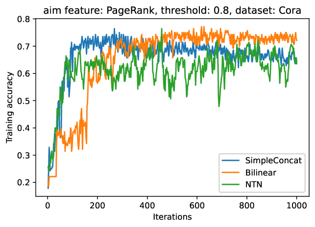
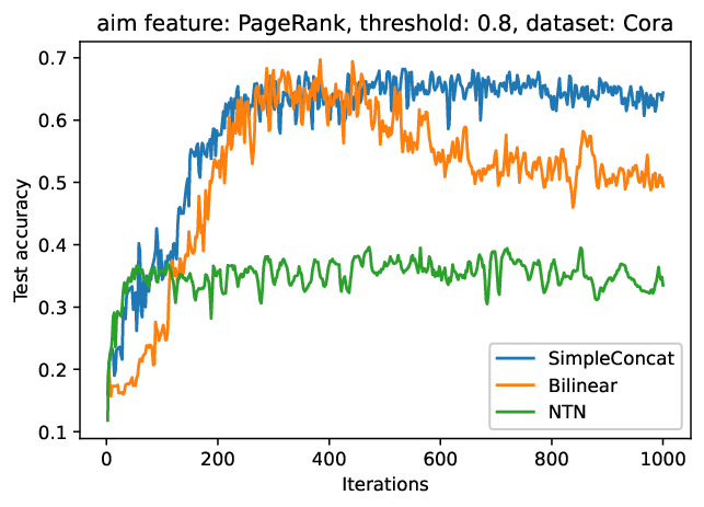
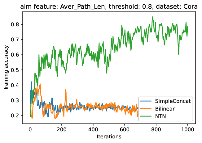
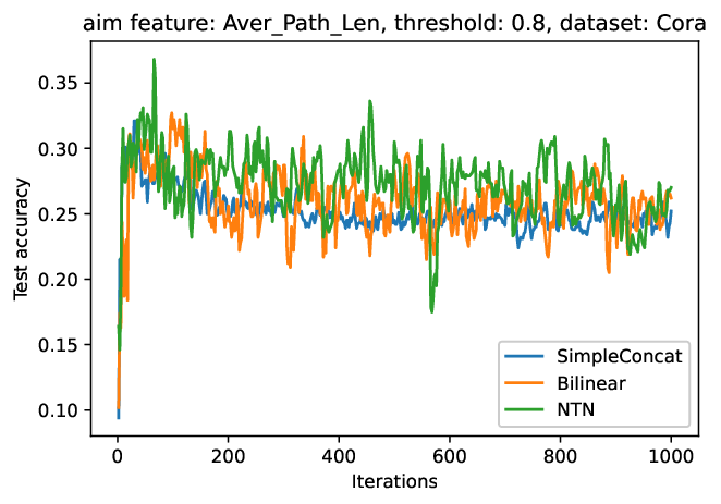
concatenation comparison NTN method is worse than simple concatenation in the process of training the predicted pagerank of Cora dataset, and it generalizes worse on test datasets. The bilinear method faces the problem of over-fitting . In general, the simple concatenation has the best performance on test datasets. When predicting average path length on Cora dataset, NTN is far better than bilinear and simple concatenation but they show similar results on test datasets. More specifically, Bilinear and NTN have a serious fluctuation problem on accuracy, overall NTN is the optimal method according to Fea2Fea-multiple. These experiments indicate that complex concatenation method such as NTN does not always have the best performance. Sometimes the simplest way is the best way.


| Aim | Citeseer | PubMed | ||||||||
|---|---|---|---|---|---|---|---|---|---|---|
| GCN | GIN | SAGE | GAT | MLP | GCN | GIN | SAGE | GAT | MLP | |
| Cons Deg | 0.587 | 1.000 | 0.379 | 0.379 | 0.379 | 0.678 | 0.996 | 0.478 | 0.478 | 0.478 |
| Deg Deg | 0.899 | 1.000 | 0.994 | 0.395 | 1.000 | 0.725 | 1.000 | 0.958 | 0.477 | 1.000 |
| Clu Deg | 0.628 | 1.000 | 0.631 | 0.492 | 0.670 | 0.643 | 1.000 | 0.603 | 0.471 | 0.574 |
| PR Deg | 0.466 | 1.000 | 0.409 | 0.376 | 0.379 | 0.539 | 1.000 | 0.600 | 0.478 | 0.478 |
| Avglen Deg | 0.536 | 0.997 | 0.686 | 0.476 | 0.473 | 0.696 | 1.000 | 0.785 | 0.478 | 0.524 |
| Cons Clu | 0.671 | 0.693 | 0.658 | 0.658 | 0.658 | 0.799 | 0.805 | 0.780 | 0.780 | 0.780 |
| Deg Clu | 0.688 | 0.714 | 0.736 | 0.658 | 0.726 | 0.794 | 0.804 | 0.804 | 0.780 | 0.805 |
| Clu Clu | 0.857 | 0.882 | 0.980 | 0.846 | 0.992 | 0.831 | 0.839 | 0.939 | 0.762 | 0.932 |
| PR Clu | 0.672 | 0.687 | 0.670 | 0.658 | 0.658 | 0.792 | 0.805 | 0.780 | 0.780 | 0.780 |
| Avglen Clu | 0.681 | 0.696 | 0.684 | 0.658 | 0.676 | 0.794 | 0.785 | 0.790 | 0.780 | 0.780 |
| Cons PR | 0.702 | 0.671 | 0.202 | 0.190 | 0.190 | 0.669 | 0.529 | 0.161 | 0.141 | 0.161 |
| Deg PR | 0.637 | 0.750 | 0.752 | 0.266 | 0.443 | 0.564 | 0.629 | 0.617 | 0.175 | 0.565 |
| Clu PR | 0.549 | 0.575 | 0.435 | 0.279 | 0.315 | 0.437 | 0.559 | 0.409 | 0.196 | 0.326 |
| PR PR | 0.192 | 0.635 | 0.415 | 0.263 | 0.190 | 0.478 | 0.554 | 0.336 | 0.161 | 0.161 |
| Avglen PR | 0.529 | 0.691 | 0.602 | 0.312 | 0.333 | 0.541 | 0.591 | 0.537 | 0.274 | 0.263 |
| Cons Avglen | 0.442 | 0.503 | 0.178 | 0.166 | 0.173 | 0.294 | 0.394 | 0.168 | 0.168 | 0.168 |
| Deg Avglen | 0.528 | 0.542 | 0.553 | 0.285 | 0.330 | 0.415 | 0.443 | 0.437 | 0.153 | 0.313 |
| Clu Avglen | 0.420 | 0.377 | 0.387 | 0.248 | 0.246 | 0.296 | 0.330 | 0.300 | 0.171 | 0.184 |
| PR Avglen | 0.268 | 0.466 | 0.207 | 0.310 | 0.173 | 0.316 | 0.459 | 0.198 | 0.197 | 0.168 |
| Avglen Avglen | 0.734 | 0.597 | 0.937 | 0.596 | 0.979 | 0.450 | 0.378 | 0.860 | 0.270 | 0.984 |
Appendix 0.E Graph Embedding Analysis
We extract graph embedding vectors and linear layer embedding vectors to perform tsne visualization and comparsion. When predicting pagerank from node degree on Citeseer dataset, the graph embedding is similiar to the mlp embedding. On Proteins dataset, graph embedding cannot separate classes well compared with mlp embedding. When performing multiple features to single featuere prediction, input embedding indicates that input features are mixed which cannot classify the class well but mlp embedding can separate the class well. It emphasizes the importance of a MLP after the GNN block.
i


Appendix 0.F generalization
We extend the results that we reach from benchmark datasets on synthetic dataset. We set up five new graph with number of nodes n {50, 200, 400, 800, 1000}. We use the same model with the same parameter settings in Fea2Fea-single. We found that the feature clustering coefficient is still the most difficult to predict and degree is the easiest to predict, which is the same as what we’ve previously found in Planetoid and TUdataset. As the number of nodes or features in the network increases, feature mutual prediction becomes more accurate.


| Aim | Number of nodes | ||||
|---|---|---|---|---|---|
| 50 | 200 | 400 | 800 | 1000 | |
| Cons Deg | 0.800 | 0.950 | 1.000 | 0.975 | 1.000 |
| Deg Deg | 0.800 | 0.950 | 1.000 | 0.975 | 1.000 |
| Clu Deg | 1.000 | 1.000 | 1.000 | 0.975 | 1.000 |
| PR Deg | 0.800 | 0.950 | 1.000 | 1.000 | 0.990 |
| Avglen Deg | 1.000 | 1.000 | 1.000 | 1.000 | 1.000 |
| Cons Clu | 0.800 | 0.750 | 0.550 | 0.650 | 0.800 |
| Deg Clu | 0.800 | 0.900 | 0.525 | 0.775 | 0.780 |
| Clu Clu | 1.000 | 0.850 | 0.675 | 0.700 | 0.850 |
| PR Clu | 0.800 | 0.800 | 0.500 | 0.762 | 0.810 |
| Avglen Clu | 0.800 | 0.700 | 0.625 | 0.688 | 0.720 |
| Cons PR | 1.000 | 0.850 | 0.850 | 0.912 | 0.910 |
| Deg PR | 0.800 | 0.900 | 0.850 | 0.912 | 0.950 |
| Clu PR | 0.600 | 0.850 | 0.825 | 0.825 | 0.930 |
| PR PR | 1.000 | 0.850 | 0.875 | 0.850 | 0.930 |
| Avglen PR | 0.600 | 0.850 | 0.825 | 0.863 | 0.890 |