On compressing sinh-Gordon solutionsPreprint: QMUL-PH-21-13

In regions where $uv=0$, eqn. (1) reduces to the Liouville equation. Outside these regions, after a coordinate transformation given by $d\tilde{\sigma}^{-}=\sqrt{|u({\sigma^{-}})|}d\sigma^{-}$, $d\tilde{\sigma}^{+}=\sqrt{|v({\sigma^{+}})|}d{\sigma^{+}}$, the equation takes the standard sinh-Gordon or cosh-Gordon form

$$\tilde{}\partial_{+}\tilde{}\partial_{-}\tilde{\alpha}+e^{\tilde{\alpha}}\pm e^{-\tilde{\alpha}}=0$$

(2)

where $\tilde{\alpha}=\alpha-\log\sqrt{|uv|}$. The variables $\tilde{\sigma}^{\pm}$ will be called balanced coordinates.

The non-linear sinh-Gordon equation is integrable Pohlmeyer 1976; De Vega and Sanchez 1993 and possesses singular soliton solutions. Multi-soliton solutions can be constructed by the inverse scattering method. In this Letter the relationship between the sinh-Gordon equation and long Nambu-Goto strings (extremal surfaces) in AdS₃ will be exploited to obtain scheme-dependent non-linear transformations which compress solution of the sinh-Gordon equation into parametrically small regions. The flowchart of the map is illustrated in FIG.1.

The string can be mapped into AdS₃ by taking the target space to be ${\mathbb{{R}}}^{2,2}$ and then forcing the string to lie on the hyperboloid using a Lagrange multiplier. In conformal gauge the action is given by

$$S=-{T\over 2}\int d\tau d\sigma(\partial_{\sigma}Y^{\mu}\partial_{\sigma}Y_{\mu}-\partial_{\tau}Y^{\mu}\partial_{\tau}Y_{\mu}+\lambda(Y^{2}+1)),$$

where $T$ is the string tension and $Y(\tau,\sigma)\in{\mathbb{{R}}}^{2,2}$ is the embedding function. The equation of motion in lightcone coordinates is

$$\partial_{+}\partial_{-}Y-(\partial_{+}Y\cdot\partial_{-}Y)Y=0\,.$$

Due to the gauge choice, the equations are supplemented by the Virasoro constraints

$$\partial_{-}Y\cdot\partial_{-}Y=\partial_{+}Y\cdot\partial_{+}Y=0\,.$$

From the string embedding the sinh-Gordon field can be computed via

$$\alpha=\log|\partial_{-}Y\cdot\partial_{+}Y|\,.$$

(3)

If the unit normal vector $N$ is defined such that

$$N_{a}=e^{-\alpha}\epsilon_{abcd}Y^{b}\partial_{-}Y^{c}\partial_{+}Y^{d}$$

then the auxiliary fields are given by

	$\displaystyle u$	$\displaystyle=$	$\displaystyle-N\cdot\partial_{-}\partial_{-}Y=\partial_{-}N\cdot\partial_{-}Y=-Y\cdot\partial_{-}\partial_{-}N$
	$\displaystyle v$	$\displaystyle=$	$\displaystyle N\cdot\partial_{+}\partial_{+}Y=-\partial_{+}N\cdot\partial_{+}Y=Y\cdot\partial_{+}\partial_{+}N$		(4)

The string equations of motion guarantee that $u=u({\sigma^{-}})$ and $v=v({\sigma^{+}})$ and that the quantities satisfy the generalized sinh-Gordon equation Pohlmeyer 1976; De Vega and Sanchez 1993. Note that while changing $N\to-N$ flips the signs of both $u$ and $v$, their product which appears in (1) remains invariant.

The segmentation procedure is depicted in FIG. 2. The diagram shows the string worldsheet (yellow surface) embedded into AdS₃. A time-slice on the worldsheet is indicated by a black line. One can discretize this curve according to any preferred scheme. This will result in a set of points $\{P_{i}\}$.

Consider the motion given by

$$x_{0}(t_{r})=\theta(\sqrt{1+t^{2}}-1)\,,$$

where $\theta$ is the Heaviside function. Mikhailov’s embedding gives a segmented string that consists of two pieces: a vertical segment at $x=0$ attached to another one with radius $R=1$. The relativistic acceleration of the string endpoint (the inverse radius of the segment) jumps as seen in FIG. 3. One can smooth the kink by choosing a new $\tilde{x}_{0}(t_{r})$ function which is equal to $x_{0}(t_{r})$ outside the region $(-{\varepsilon\over 2},{\varepsilon\over 2})$ and whose acceleration is smooth (red dashed line in the figure). The average slope of the acceleration function will be of the order of $\Delta a/\varepsilon$ where $\Delta a$ is the jump in the acceleration. In order to have an estimate for the $u$ field across this region, the smooth motion of the endpoint can be approximated by taking $\tilde{x}_{0}(t_{r})={\Delta at_{r}^{3}/\varepsilon}$ which will produce a linear acceleration function for small positive $t_{r}$. After changing to lightcone coordinates in Mikhailov’s embedding, one gets $u\approx{6\Delta a/\varepsilon}$. This means that in balanced coordinates the width of the smoothed kink is (see FIG. 4)

$$L\propto\sqrt{u}\,\varepsilon\propto\sqrt{\Delta a\varepsilon}\,.$$

If there are $N$ segments, then $\Delta a$ scales as $N^{-1}$ and $\varepsilon$ can also be taken to scale in the same way. The balanced linear size on the worldsheet is then proportional to $N^{0}\sqrt{\varepsilon}$.

In the final step of the transformation, the sinh-Gordon fields $\alpha,u,v$ are computed. As $N\to\infty$, the segmented string approaches the original smooth string and thus their time evolution will be the same.

In order to compress the function, the first step is constructing the corresponding string embedding. The spinor solutions of (5) are found to be

	$\displaystyle\psi^{L}_{1}$	$\displaystyle=$	$\displaystyle e^{\omega_{-}}\left(\sqrt{\frac{2}{\text{sn}}+2k\,\text{sn}},\ -\frac{\sqrt{2}\left(\text{cn}\,\text{dn}+\text{sn}\sqrt{k^{2}-1}\right)}{\sqrt{\text{sn}+k\text{sn}^{3}}}\right)$
	$\displaystyle\psi^{L}_{2}$	$\displaystyle=$	$\displaystyle e^{-\omega_{-}}\left({\sqrt{\frac{1+k\text{sn}^{2}}{8\text{sn}\left(k^{2}-1\right)}}},\ \frac{\text{sn}\sqrt{k^{2}-1}-\text{cn}\,\text{dn}}{\sqrt{8\left(k^{2}-1\right)\left(\text{sn}+k\text{sn}^{3}\right)}}\right)$
	$\displaystyle\psi^{R}_{1}$	$\displaystyle=$	$\displaystyle e^{\omega_{+}}\left(-\frac{\sqrt{2}\left(\text{cn}\,\text{dn}+\text{sn}\sqrt{k^{2}-1}\right)}{\sqrt{\text{sn}-k\text{sn}^{3}}},\ \sqrt{\frac{2}{\text{sn}}-2k\,\text{sn}}\right)$
	$\displaystyle\psi^{R}_{2}$	$\displaystyle=$	$\displaystyle e^{-\omega_{+}}\left(\frac{-\text{sn}\sqrt{k^{2}-1}+\text{cn}\,\text{dn}}{\sqrt{8\left(k^{2}-1\right)\left(\text{sn}-k\text{sn}^{3}\right)}},\ -{\sqrt{\frac{1-k\text{sn}^{2}}{8\left(k^{2}-1\right)\text{sn}}}}\right)$

where

	$\displaystyle\Pi_{\pm}$	$\displaystyle\equiv$	$\displaystyle\Pi\left(\pm k;\text{am}\left(\frac{\sigma}{\sqrt{2k}}|-k^{2}\right)|-k^{2}\right)$
	$\displaystyle\omega_{\pm}$	$\displaystyle\equiv$	$\displaystyle\sqrt{k-k^{-1}}\left(-\sqrt{k}\Pi_{\pm}+{\tau+\sigma\over 2\sqrt{2}}\right)$

and sn, cn and dn denote Jacobi elliptic functions with arguments $\left(\frac{\sigma}{\sqrt{2k}}|-k^{2}\right)$, and am is the Jacobi amplitude function. If one eliminates $\tau$ in favor of Poincaré time $t$, then the embeddings will have the form $x(\sigma,t)=t\,\tilde{x}(\sigma)$ and $y(\sigma,t)=t\,\tilde{y}(\sigma)$. Thus they scale linearly with time while their shape is constant.

The shape $\tilde{x}(\tilde{y})$ of such an embedding satisfies the equation of motion

$$\tilde{y}\left(\tilde{x}^{2}+\tilde{y}^{2}-1\right)\tilde{x}^{\prime\prime}+\left(2-2\tilde{y}^{2}\right)\tilde{x}^{\prime 3}+4\tilde{x}\tilde{y}\tilde{x}^{\prime 2}+\left(2-2\tilde{x}^{2}\right)\tilde{x}^{\prime}=0$$

which can be derived from the Nambu-Goto action. FIG. 6 (left) shows the embedding on the Poincaré patch for various values of $k$. As $k\to 1^{+}$, at $t=1$ the string is mapped into a vanishingly small region near the origin and its size increases slowly as time evolves. By applying an $SO(2,2)$ isometry transformation the size of the string can be kept finite as the limit is taken. Thus at $k=1$ the string is static. In the following, let us concentrate on this special case. Its shape $x(y)$ satisfies the equation

$$2x^{\prime}+2(x^{\prime})^{3}-yx^{\prime\prime}=0$$

which is indeed invariant under rescaling the coordinates by a constant factor. The explicit solution centered at $x=0$ has two branches⁵⁵ 5 The Ricci scalar of the induced metric is $R=-2\left(1+(y/y_{0})^{4}\right)$. Since $R<R_{0}$ (where $R_{0}=-2$ is the curvature of AdS₃) the solution in balanced coordinates satisfies the cosh-Gordon equation. Close to the boundary ($y\to 0$) the solution asymptotes to AdS₂.

$$x(y)=\mp x_{0}\pm{y^{3}\over 3y_{0}^{2}}\,_{2}F_{1}\left({\frac{1}{2},\frac{3}{4};\frac{7}{4}};{y^{4}\over y_{0}^{4}}\right)$$

where $x_{0}\equiv\frac{\sqrt{\pi}\Gamma\left(\frac{7}{4}\right)}{3\Gamma\left(\frac{5}{4}\right)}y_{0}$ and $y_{0}$ is a parameter. The string touches the boundary at $x=\pm x_{0}$. In FIG. 6 (middle) the embedding is plotted (background gray curve).

The next step is to segment the string. Since in an appropriate frame the string is static, one can apply the shooting technique described in Appendix B of Vegh 2021. The only parameter is the number $N$ of string segments. The resulting segmented string is periodic in Poincaré time. An example with $N=13$ is depicted in FIG. 6 (middle). The black curves are circular arcs given by (8). Red and black dots indicate left- and right-moving kinks between the segments.

The third step is smoothing the segmented string. This can be done in the way described earlier, but in practice it is easier to do the following. One can subdivide the string into many pieces by adding “null kinks” Vegh 2016 which do not further break the individual segments (i.e. they have the same parameters in (8)). If each segment is subdivided into $n$ pieces then one has $nN$ segments in total. After the subdivision, a smoothing filter can be applied on the points. For instance one can repeatedly apply the transformation

$$P_{i}^{\prime}\propto\lambda(P_{i-1}+\lambda P_{i+1})+P_{i}\quad\textrm{such that}\quad(P_{i}^{\prime})^{2}=-1\,,$$

for points in the refined segmented string, and the same for $Q_{i}$. This step smoothes the points similarly to a discretized heat equation. After an iteration $Q^{\prime}_{i}-P^{\prime}_{i}$ and $Q^{\prime}_{i}-P^{\prime}_{i+1}$ are generically not null, but one can define new $Q^{\prime\prime}_{i}$ positions such that they lie in the AdS₂ spanned by $\{P^{\prime}_{i},Q^{\prime}_{i},P^{\prime}_{i+1}\}$ and that $(Q^{\prime\prime}_{i}-P^{\prime}_{i})^{2}=(Q^{\prime\prime}_{i}-P^{\prime}_{i+1})^{2}=0$, and the points $P^{\prime\prime}_{i}=P^{\prime}_{i}$ are not changed. In the next iteration one smoothes the initial data given by the null zigzag $\{P^{\prime\prime}_{i},Q^{\prime\prime}_{i}\}$. Let $q$ denote the number of smoothing iterations on the string. For sufficiently large $n$, the resulting string is a good approximation for a smooth string. An example is depicted in FIG. 6 (right).

Finally, the generalized sinh-Gordon fields $\alpha,u,v$ can be computed using worldsheet points and normal vectors which all take values in ${\mathbb{{R}}}^{2,2}$. For instance in FIG. 7 for the patch with normal vector $N_{1}$ one has

$$e^{\alpha}=a^{-2}(V_{10}-V_{00})(V_{01}-V_{00})$$

(10)

where $a$ is the lattice spacing. A discrete version of (4) is given by

$$v\approx a^{-2}(N_{1}-N_{2})(V_{01}-V_{00})$$

(11)

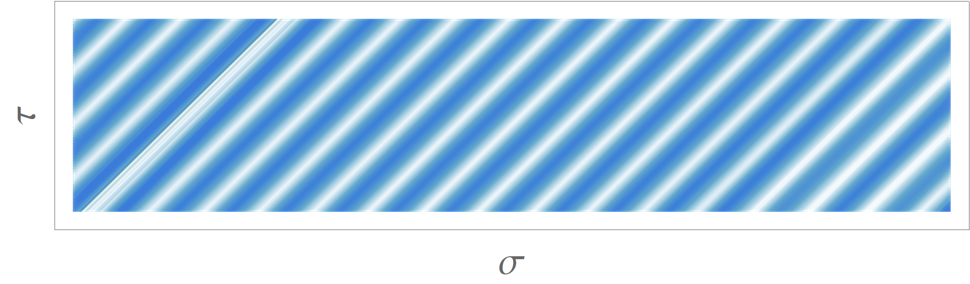
and an approximate $u$ function can similarly be computed. FIG. 8 (middle) shows an example for $v$ computed this way for a slightly smoothed string with $N=30$ segments. After switching to balanced coordinates, the cosh-Gordon field is seen to have peaks traveling with the speed of light, see FIG. 8 (bottom). Time-slices are show in FIG. 9. For comparison, the original potential given in (9) with $k=1$ is plotted in black. The difference between the two figures is the number of smoothing iterations applied on the subdivided segmented string. Without any smoothing the balanced width of the string would be zero and the spikes would diverge.

Finally, one can check that the balanced width $L$ of the compressed function indeed scales as expected. Based on the properties of the heat equation, one expects that an appropriate smoothing parameter can be defined as $\varepsilon=\sqrt{q}/n$ and that $L\propto\sqrt{\varepsilon}$. This is indeed born out by numerical calculations: for an example with $N=10$ segments a numerical fit gave $L\propto n^{\gamma}$ with $\gamma=-0.495\pm 0.01$ and $L\propto q^{\delta}$ with $\delta=0.246\pm 0.01$, confirming the expectations.

For the transformation, one can use various segmentation and smoothing schemes. In a given scheme one is still left with two parameters: the number of string segments $N$, and the smoothing parameter $\varepsilon$. It is plausible that in an appropriate large-$N$ limit the scheme-dependence goes away. It would be interesting to see if one can define the transformation in a closed form similarly to an auto-Bäcklund transformation.

The equations of motion for a string in AdS₃ have an internal $SO(2,2)$ symmetry acting on the vectors $\{Y,e^{-{\alpha\over 2}}\partial_{-}Y,e^{-{\alpha\over 2}}\partial_{+}Y,N\}$ Alday and Maldacena 2009. Note that this symmetry has been broken by both smoothing procedures discussed in the paper.

The results made use of the equivalence of the sinh-Gordon equation and the string equation of motion in AdS₃. Similar equivalences exist in higher dimensional AdS spacetimes which allows for the extension of the compressing transformation to other systems, such as the $B_{2}$ Toda theory which is related to strings moving in AdS₄ Jevicki and Jin 2010.

The transformed function contains $N$ peaks which superficially look similar to boosted sinh-Gordon solitons. Solitons can be thought of as particles whose motion is governed by the hyperbolic Ruijsenaars-Schneider model with a special coupling value Ruijsenaars and Schneider 1986. Since the balanced size of the transformed domain vanishes as $\varepsilon\to 0$, it is plausible to think that this gives an interesting limit of the model. Perhaps this limit leads to a dual description of the string.

References

- Pohlmeyer (1976) K. Pohlmeyer, Commun. Math. Phys. 46, 207 (1976).
- Gross and Neveu (1974) D. J. Gross and A. Neveu, Phys. Rev. D 10, 3235 (1974).
- Neveu and Papanicolaou (1978) A. Neveu and N. Papanicolaou, Commun. Math. Phys. 58, 31 (1978).
- De Vega and Sanchez (1993) H. J. De Vega and N. G. Sanchez, Phys. Rev. D47, 3394 (1993).
- Alday and Maldacena (2009) L. F. Alday and J. Maldacena, JHEP 0911, 082 (2009), eprint 0904.0663.
- Jevicki et al. (2008) A. Jevicki, K. Jin, C. Kalousios, and A. Volovich, JHEP 0803, 032 (2008), eprint 0712.1193.
- Vegh (2018) D. Vegh, JHEP 02, 045 (2018), eprint 1508.06637.
- Callebaut et al. (2015) N. Callebaut, S. S. Gubser, A. Samberg, and C. Toldo, JHEP 11, 110 (2015), eprint 1508.07311.
- Gubser et al. (2016) S. S. Gubser, S. Parikh, and P. Witaszczyk, JHEP 07, 122 (2016), eprint 1602.00679.
- Vegh (2016) D. Vegh (2016), eprint 1601.07571.
- Vegh (2021) D. Vegh, JHEP 03, 218 (2021), eprint 1802.04306.
- Mikhailov (2003) A. Mikhailov (2003), eprint hep-th/0305196.
- Jevicki and Jin (2010) A. Jevicki and K. Jin, JHEP 03, 028 (2010), eprint 0911.1107.
- Ruijsenaars and Schneider (1986) S. N. M. Ruijsenaars and H. Schneider, Annals Phys. 170, 370 (1986).