Virtual Point Source Synthesis method for 3D Scintillation Detector Characterization
Abstract
A novel data-processing method was developed to facilitate scintillation detector characterization. Combined with fan-beam calibration, this method can be used to quickly and conveniently calibrate gamma-ray detectors for SPECT, PET, homeland security or astronomy. Compared with traditional calibration methods, this new technique can accurately calibrate a photon-counting detector, including DOI information, with greatly reduced time. The enabling part of this technique is fan-beam scanning combined with a data-processing strategy called the common-data subset (CDS) method, which was used to synthesize the detector’s mean detector response functions (MDRFs). Using this approach, scans ( in x and in y direction) are necessary to finish calibration of a 2D detector as opposed to scans with a pencil beam. For a 3D detector calibration, only scans are necessary to achieve the 3D detector MDRFs that include DOI information. Moreover, this calibration technique can be used for detectors with complicated or irregular MDRFs. We present both Monte-Carlo simulations and experimental results that support the feasibility of this method.
Index Terms:
Photon-counting, detector, calibration, depth of interaction (DOI), digital signal processing, SPECT, PET.I Introduction
Since its invention in 1952, the Anger camera and its derivatives have been widely used in gamma-ray imaging applications such as SPECT and PET, with “Anger arithmetic” used as the standard method for gamma-ray interaction position estimation[1][2]. However, this method exhibits large bias or variance in estimated positions, especially at areas close to detector edges. Reference-data based methods have been developed, which have better positioning performance over Anger arithmetic. These methods include, but are not limited to, maximum likelihood estimation (MLE)[3], artificial neural networks (ANNs)[4, 5, 6, 7, 8, 9], K-nearest neighbors (KNNs)[10] and k-d tree search[11]. All of these methods require detectors to be calibrated to acquire reference data, which is subsequently used in gamma-ray interaction position estimation. The calibration or collection of reference data is usually performed using a well-collimated, normally-incident pencil beam of gamma rays to scan positions across the entrance surface of the detector and collecting a fixed number of events at each of these positions[12]. This process can be very time-consuming, especially when the collimated beam diameter and step size are relatively small when calibrating high-resolution or large-area detectors. Newly proposed calibration methods include using two perpendicular fan beams[13]; calibrating the detector with uncollimated gamma-ray sources after which algorithms are used to estimate the reference data[14]; and generation of reference data by careful detector modeling[15]. Despite various available methods, the DOI calibration of thick photon-counting detectors still remains a challenge[16, 17, 18]. A method that combines both efficiency and DOI capability is still needed. The introduced method, which has been briefly introduced in the preceding simulation work[19], takes off difficulty from the calibration process and places more burden on the data processing side, and it is capable of carrying out a 2D and 3D calibration (with DOI capability) of photon-counting detectors using two and three fan-beam scans, respectively. Moreover, by combining this DOI-enabled fast calibration methods with fast gamma-ray event position estimation methods such as k-d tree search [11] or contracting-grid search [20], broader application of monolithic gamma-ray detector might be possible.
In this work, we proposed a fan-beam data processing method called the common-data subset (CDS) method, which could enable the DOI calibration of a monolithic crystal detector with reduced time. Both simulation and experiment are shown to validate this method.
II Materials and methods
II-A Basis of common data subset (CDS) calibration
The basic idea of this calibration method is to use algorithms to find the events located at the overlapping positions of any intersecting fan beams.
II-A1 Two-dimensional (2D) calibration
As an example, a detector is first scanned by a vertical fan beam moving along x direction; and then a horizontal beam is used to scan the detector along y direction. For both horizontal and vertical directions, the fan beam stops at positions and reference data is collected at each of the positions (Fig. 1).

scans are collected in each of the two directions as shown in Fig. 1. Each of the scans includes certain number of gamma-ray interaction events, which form a reference dataset, therefore there are in total reference datasets collected as Fig. 1 shows. In this work, we define that an event in one dataset represents the signals of all the detector’s light sensors produced by a single gamma-ray interaction (1).
| (1) | ||||
is the index of a single event in a reference dataset, and is the index of datasets (for example, index of the datasets along x direction, Fig. 1). Assuming that the detector has a total of light sensors, then each reference event (vector) has signal components. Two gamma-ray interactions that occur in close proximity inside the detector will give two similar signal responses. We assert the opposite is also true, namely that:
If two gamma-ray interactions yield similar signal responses, their interaction positions in the photon-counting detector are close to each other.
This assumption is true if the detector is well-designed so that the interaction positions and their mean signal responses have one-to-one mapping relationships, while a poorly-designed detector has the same signal responses even for events interacting at different positions, thus causing position-estimation ambiguity when using the signal response of an event to estimate the event’s position of interaction. Suppose there are two calibration datasets and acquired by two orthogonal fan beams. Then we search for the data subsets and such that (meaning that the two event subsets have similar events compared with each other). Dataset is defined to be the common-data subset (CDS) of datasets and . Considering the above assumption, the common-data subset contains the gamma-ray events that interact inside or close to the overlapping volume of the two calibration fan beams.
If the CDS of two datasets can be found using algorithms, the calibration datasets could effectively generate what would be produced by a pencil beam (Fig. 2).

After all of the reference datasets of the fan beam scanning horizontally are acquired and represented as {} = {}, and all the reference datasets of the fan beam scanning vertically are also acquired and represented as {} = {}, different combinations of and yield an grid of calibration datasets that can be used to generate the detector signal responses or mean detector response functions (MDRFs) – the mean signal map of each light sensor of the detector, as a function of gamma-ray interaction position in the detector volume.
Using this method, only fan-beam scans are necessary, that greatly cut down the calibration time, as opposed to that of scans using a pencil beam. Making a well-collimated fan beam is much easier than making a well-collimated pencil beam, especially for high-energy gamma rays.
II-A2 Three-dimensional (3D) detector calibration
Analogously to the 2D detector case, in order to calibrate the 3D signal responses (3D MDRFs) for a thick detector, only scans by a fan beam are necessary, as illustrated in Fig. 3.

The first two orthogonal fan beams are used to produce the CDSs whose corresponding interaction locations are located at or close to the overlapping detector volume of the two fan beams, which defines a tubular volume (red area in Fig. 3). The third calibrating beam is used to intersect the tubular segment to define a small volume (similarly, the intersection of three planes is a point). By translating the three fan beams, the whole 3D detector volumes can be calibrated, then the 3D MDRFs can be derived based on different combinations of the achieved datasets.
In this case, the DOI calibration can be performed easily and conveniently. DOI estimation could help PET system to improve radical spatial resolution close to edges of field of view (FOV) and help pin-hole SPECT system to reduce parallax errors near edges of detectors. In most cases, the third fan beam can be orthogonal to the first and second fan beams which is often preferred due to its simplicity. However, for some specific scenarios, using a slant third beam is more beneficial. For example, if a monolithic SPECT detector has a large and flat scintillation crystal (large entrance surface, with small thickness), a third beam orthogonal to the first and second beams will be perpendicular to the edge surface of the scintillation crystal, and its travel distance inside the scintillation crystal will be relatively long, leaving very few interaction events where the beam exits the crystal, thus the statistic noise will be higher. If using a slant beam, the attenuation effect would be greatly mitigated due to a shorter travel distance inside the crystal.
II-B Algorithm for finding the common data subset (CDS) of two datasets
The basic mathematical task is to efficiently find the common data subset (CDS) of two datasets under the influence of noise. Virtually no event (signal vector) in dataset will be exactly identical to any event in dataset . However, the events in dataset , that are similar to one or more events in dataset could be found out.
| (2) |
And similarly, will be found according to (3).
| (3) |
Then the common data subset (CDS) can be formed by taking the union of the above two datasets.
| (4) |
To quantify if an event in dataset is “similar” or “close” to a particular event in dataset , a score should be defined. Because each event’s signal vector has components (where represents the number of light sensors or readout channels of the detector), each event is a signal vector . The closeness of an event in dataset to dataset can be, for example, quantified by the following score equation.
| (5) |
Where in the above equation is a tunable constant, which represents the radius of the field extended by each reference event in . Each event in the reference dataset extends a field in dimensional space, and the summation of all the field values in a specific location (decided by the query event) in the dimensional space defines the score value of that event. For the above score definition, the shape of field is Gaussian. This value needs to be tuned, since if is too large, the resolution of the CDS method will be poor, so events outside the intersection volume of the two beams might be mixed into the common-data subset (CDS). But if is too small, the radius of the field extended by each reference event will be too small, so the score of an event located at the common volume will sometimes have very small score value, which could be excluded from the CDS; while an event outside the common volume could be wrongly included into the CDS if it happens to have a higher score value under the influence of noise. This example shows only one of many available options to define the score, other definitions could be possible, such as changing the power of 2 in equation (5) to 1, 3, or 4…
In order to find the CDS of two datasets and : first, calculate the score of across all the datasets ; find the dataset in that gives the highest score; then assign to that dataset, and the event ’s coordinate of the direction along which datasets are collected can be achieved. Repeat the same procedure for other directions, then the 3D coordinate of event can be achieved. All events in the reference datasets can be processed in this way, and we call this method the “competitive method”. By default, we will use this method for the rest of this work.
Once the CDSs are achieved, the events in the reference datasets can be associated with their interaction positions in the detector volume, and the corresponding MDRF value, namely , can be calculated easily by averaging the signal vectors of all the events in the CDS of location , where is the index of light sensors.
After calculating the MDRFs, the estimated location of a query event can be found using maximum likelihood position estimation[3].
| (6) | ||||
II-C Simulation
II-C1 Simulation of a thick monolithic PET detector
The geometry of a simulated detector is shown in Fig. 4. The detector is composed of a thick LYSO scintillation crystal (mmmmmm, refractive index is ), a light guide made of glass (mmmmmm, refractive index is ), and SiPMs of dimensions mmmm with sensitive area of mmmm, forming a array on bottom of the light guide. The window material of the SiPMs has a thickness of um and a refractive index of . The photon detection efficiency (PDE) of the SiPMs was modeled to be %. The SiPMs’ dark count rate is MHz/mm2, and excess noise factor (ENF) was modeled to be to avoid overly-optimistic result. All the parameters of the simulated SiPMs were chosen conservatively within the scope of current industrial capability [21, 22]. The entrance surface of the detector is a Lambertian reflector, with reflectance of %, while the side walls of the detector are black absorber, with reflectance of %. Optical gel of refractive index of was modeled as the optical coupling medium between the light guide and the SiPMs, and its thickness is um. The surfaces of the SiPMs were modeled to be specular surfaces with % reflectance. The LYSO crystal’s light yield was modeled to be photons/MeV[23], with its intrinsic energy resolution modeled to be %, its attenuation length () for keV gamma rays is mm, while its optical attenuation length () is cm[24]. The simulation is done using C++, and data processing of CDS is done using C++/CUDA.
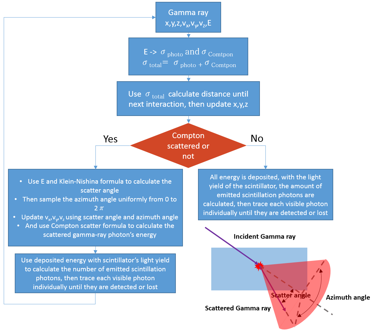
In order to study the impact of Compton effect, we first simulated without considering Compton effect by letting each interacting gamma-ray photon interact by photoelectric effect. After that, we carried out another simulation including Compton effect. At last, we compared the results with and without Compton effect. The flow chart of how each gamma-ray photon is simulated is shown in Fig. 5. Each gamma ray is modeled as follows:
1. Each gamma-ray photon can be described by its positon , its direction , and its energy . The energy of a single gamma-ray photon is used to get its corresponding Compton scattering and photoelectric cross sections ( and ), and the total interaction cross section is the sum of Compton scattering and photoelectric cross sections.
2. A random number is used together with the total interaction cross section to determine how far this gamma-ray photon can travel before interacting with the scintillation material. Then the position of this gamma-ray photon is updated with this new interaction position.
3. Another random number is used to determine whether this gamma-ray photon interacts with scintillator by Compton or photoelectric effect. If the gamma-ray photon interacts by Compton effect, the scattering angle of scattered photon is sampled from the pre-stored look-up table (LUT) calculated using Klein-Nishina formula [25]. The LUT is a two-dimensional matrix, with its row axis indicating the incident gamma ray’s energy, and the column axis indicating the scattering angle. The value in the matrix indicates the probability of each scattering angle, given a gamma ray’s incident energy, so each row of the matrix represents the scattering angle’s probability density function. After the scattering angle is achieved by sampling from the LUT, the azimuth angle is sampled uniformly from to , then the direction vector of the scattered gamma-ray () is fully determined, and the scattered gamma-ray photon’s energy is calculated using the Compton formula. The energy deposited locally by Compton effect is then known, which is used to calculate the number of emitted visible photons by the scintillator, and each visible photon is traced until it is either detected or absorbed internally without being detected. Then go back to step 1, and repeat the whole process for the scattered gamma-ray photon.
4. If the gamma-ray photon interacts by photoelectric effect, all of its energy is deposited locally at the interaction position, and visible photons are emitted. Each visible photon is traced until it is either detected or absorbed internally without being detected, then the simulation of this particular gamma-ray photon is done.

Three fan beams are simulated to scan across the detector, as shown in Fig. 6.

A fan beam (mm FWHM) scanned the detector along x direction, then the fan beam was rotated , and scanned the detector along y direction. After that, the beam is inclined at angle with respect to entrance surface of the detector and scanned the detector along x direction. The fan beam each stopped at locations along the scintillation crystal when scanning along x and y direction, with a step size of mm, starting/ending at mm (half pitch size) from the side surfaces of the crystal. When scanning with a slant angle, the fan beam stopped at locations, with step size of mm along x direction. At the starting point, the slant fan beam intersected the side surface of the scintillation crystal at mm from the bottom surface. At the ending point, the slant beam intersected the crystal’s top surface at mm from the side surface. For simulation excluding Compton effect, at each scanned location, of keV gamma photons were emitted, while for simulation including Compton effect, at each scanned location, events were emitted to compensate for the loss after applying an energy window to filter out Compton-scattered events that deposit partial energy. The detected events at each scanned location form a dataset. So there were datasets formed by the fan beam scanning along x direction, datasets formed by the fan beam scanning along y direction, and datasets formed by the slant fan beam scanning along x direction. For each gamma-ray interaction inside the scintillation crystal, a burst of visible scintillation photons was emitted. The number of emitted visible photons was calculated by the amount of energy deposited, the light yield of scintillation crystal and the intrinsic energy resolution of scintillation crystal. Each visible photon was traced until it was either detected or absorbed without being detected.
After the datasets were achieved, the MDRFs of the scintillation detector were calculated using the CDS method introduced in section II, part B. That is: for each event, find the dataset with highest score among all the datasets scanning the detector along a particular direction (x, y or slant beam scanning x direction). Then the coordinate of this event can be decided. The same procedure was repeated for all the events, and the MDRF values associated with a particular voxel can be calculated by averaging all the signal vectors of events in that voxel.
The above process was repeated for the simulation including Compton effect, to see if the CDS method fails under the influence of Compton effect.
After the MDRFs were calculated with the CDS method, another set of MDRFs achieved from scanning a point source inside the detector was used for comparison (ground truth). photoelectric gamma-ray interactions were recorded at each of the grid points, and the same dataset was also used as test events to compare each event’s true position and estimated position using MDRFs, to access the accuracy of the MDRFs.
II-C2 Simulation of an edge-readout detector
This time, the simulated detector is the edge-readout detector[26] (Fig. 7). Its scintillation material was modeled to be CsI(Tl) of dimension mmmmmm, the light yield of CsI(Tl) crystal was modeled as photons/MeV[23]. SiPMs were assembled on the four edges of the CsI(Tl) crystal layer, and pieces were attached on each edge. The dimension of each SiPM was mmmm with active area of mmmm. Since the SiPM active area’s height is mm, and CsI(Tl) crystal’s thickness is mm, about half of each SiPM’s active area was not used. The simulation geometry is the same as that in the experiment section (section II, part D).
A grid of drilled-hole optical barriers was simulated[26]. Each hole’s surface was modeled as diffusive cylindrical surface which is semitransparent with absorption coefficient of %, its diameter is mm and height is mm . The distance between two adjacent optical barriers is mm.
The photon detection efficiency (PDE) of the SiPMs was modeled as % (considering the mismatch between the peak PDE wavelength of SiPM and CsI(Tl) peak emission wavelength), and the reflectance of the SiPMs was modeled as %. Between the scintillation crystal and the SiPMs, a um-thick layer of optical gel with refractive index of was modeled. The dark count rate of each SiPM was assumed to be MHz/mm2. The excess noise factor (ENF) was modeled as . Again, all the SiPM parameters in the simulation were chosen conservatively according to the major manufacturers’ data sheet [21, 22]. The simulation was done using C++, and CDS data processing is done using C++/CUDA.
Two orthogonal fan beams (mm FWHM) were modeled to scan the 2D detector along x and y directions sequentially across an area of mmmm. locations were scanned for each direction, with a step size of mm. The energy of the gamma-ray beam was modeled as keV (produced by Cs-137) and gamma-ray interactions were launched at each of the scanned locations. Again, the simulation parameters were chosen to be the same as the experiment section (section II, part D).

The 2D MDRFs of the edge-readout detector were calculated using the CDS method introduced in section II, part B. After that, another set of MDRFs were simulated by scanning a Gaussian beam of keV photons (FWHM is mm) across locations inside the edge-readout detector, and this set of MDRFs were used for comparison. The set of events generated with this Gaussian beam was also used as test events, whose real interaction positions were later compared with estimated interaction positions achieved using MDRFs.
II-D Experimental verification
The experiment used the edge-readout detector with drilled-hole optical barriers[26], whose geometry is the same as the above simulation section (section II, part C), with the width of the fan beam measured to be mm FWHM. The calibration was performed by scanning the detector at positions along horizontal direction. After that, the beam was rotated by and another scans were collected along vertical direction. The step size was mm, with events with full energy deposition collected at each position. The energy window was chosen to be %[26]. The experiment setup is shown in Fig. 8.

After collection of the datasets, the CDS method (section II, part B) was used to generate the 2D MDRFs. The CDS-generated MDRFs were then compared with the MDRFs measured using the conventional pencil beam method, which was realized by crossed-slits method using the same slits making the fan beams, which gave a spot size of mmmm FWHM at detector surface.
The event data achieved by a keV pencil beam created with crossed slits has a high variance due to aperture leakage and scattering. MDRFs are therefore calculated via an iterative filtering process at each scanning position. The steps are: 1) the mean of the signal vector is calculated; 2) each event vector’s Euclidean distance to the mean is calculated; 3) the events with the largest % Euclidean distance are eliminated; 4) loop back to step 1. This process is repeated until the result converges, for example, each events’ Euclidean distance to mean is lower than a preset threshold. At convergence, the fraction of the events contained in the calculation of the MDRF value at each scanning position is around % of the initial number of events. However, the iterative filtering method could introduce bias at the place where the MDRF gradient is high (like positions close to optical barriers).
In order to make a thorough comparison of the CDS and pencil-beam calibration methods, the events of several slit beams at different positions were estimated using the MDRFs achieved by the two methods. horizontal and vertical line images were estimated using maximum-likelihood method, each of the horizontal and vertical lines has a beam width of mm and contains gamma-ray interaction events (full energy deposition). The lines were equally-spaced with a spacing of mm. The central line is aligned with the center of the detector.
III Results
III-A Simulation of a thick monolithic detector
The 3D MDRFs generated by scanning a simulated point light source inside the scintillation crystal is shown in Fig. 9. Only three sets of MDRFs at three different depths are shown. And these MDRFs are used as ground truth.


Using the above sets of MDRFs to estimate the positions of events in the test dataset (the same dataset generated by scanning the scintillator with point light source) and comparing the estimated interaction position and the real interaction position of each event, the bias, standard deviation and root mean square error maps (in x, y and z directions) are shown in Fig. 10.


III-A1 Simulation excluding Compton effect
The CDS-generated MDRFs without considering Compton effect of the thick scintillation crystal detector of section II, part C(1) is shown in Fig. 11. Again, only three representative sets of MDRFs at three different depths are shown.


If we subtract Fig. 9 from Fig. 11, and calculate the difference relative to the maximum value in the ground truth MDRF (Fig. 9), an error map can be created, as shown in Fig. 12, the color bar is in logarithmic scale.


The mean and maximum errors of each error map are listed in TABLE I below.
![[Uncaptioned image]](2106.12219v1/table1_N3_new.png)
Using the MDRFs in Fig. 11, the positions of the test events were estimated and compared with their corresponding true positions. The bias, standard deviation and root mean square error maps are shown in Fig. 13.


III-A2 Simulation including Compton effect
Due to the fact that Compton effect can cause gamma-ray photon energy to be deposited partially, these partial-energy events need to be filtered out. Example of a histogram showing distribution of detected visible photon number is presented in Fig. 14. The events making this histogram are from a dataset of the fan beam scanning the detector center along x direction. There are in total events in this dataset for better illustration. An energy window of keV, which corresponds to detected photons in Fig. 14, was used to filter out the partial energy events.

After filtering out the partial-energy events, the datasets were used to calculate the MDRFs using the CDS method. The MDRFs achieved are shown in Fig. 15.


By comparing Fig. 15 with Fig. 9, the error maps can be calculated. Those error maps are shown in Fig. 16.


![[Uncaptioned image]](2106.12219v1/table2_N2_new.png)
Using the MDRFs in Fig. 15, the positions of the test events were estimated and compared with their corresponding true positions. The bias, standard deviation and root mean square error maps are shown in Fig. 17.


III-B Simulation of an edge-readout detector
The MDRFs generated using a traditional scanning pencil-beam method are shown in Fig. 18 (top). The MDRFs generated using the CDS method are shown in Fig. 18 (middle). The logarithmic error maps are shown in Fig. 18 (bottom), with its corresponding mean and maximum value shown in TABLE III.


![[Uncaptioned image]](2106.12219v1/table2.png)
After estimating the test events’ positions using the MDRFs, the estimated positions were compared with their corresponding true positions. The bias, standard deviation and root mean square error maps are shown in Fig. 19.

III-C Experimental result for edge-readout detector
The MDRFs acquired by scanning the pencil beam generated with the crossed-slits method are shown in Fig. 20 (top). The MDRFs generated using the CDS method are shown in Fig. 20 (middle). The error maps are shown in Fig. 20 (bottom), with its corresponding mean and maximum value shown in TABLE IV.


![[Uncaptioned image]](2106.12219v1/table3.png)
Since it is impossible to use an infinitely thin pencil beam to generate test events experimentally, accurate error maps cannot be generated. Instead, slit beams were used to quantify the accuracy ( horizontal beams and vertical beams). The estimated positions of the beam interaction events were binned into images. The images using events estimated with MDRFs achieved by conventional pencil-beam method are shown in Fig. 21, while the ones using events estimated with MDRFs achieved by CDS method are shown in Fig. 22. Note that before using those events for CDS data processing, an energy window was first used to filter out events that deposit partial energy, and the remaining events’ positions were estimated with exhaustive search method using likelihood as a metric (Maximum-likelihood estimation method[3]). At last, a likelihood threshold is used to filter out events with a lower likelihood (such as events that scatter multiple times in the detector).
If using the each event’s estimated position in Fig. 21 as ground truth, the standard deviation of events in Fig. 22 away from events in Fig. 21 along the x and y directions are um and um respectively (by comparing pair-wisely).


IV Discussion and conclusion
The simulation result of the thick monolithic detector shows CDS method’s capability of achieving DOI calibration. The maximum MDRF error according to TABLE I (without considering Compton effect) is 3.05%. Maximum MDRF error according to TABLE II (considering Compton effect) is 20%, since Compton effect might cause a gamma-ray photon to deposit energy at multiple locations, thus blurring the MDRFs, therefore error is larger at locations with high MDRF gradient. According to the estimated interaction position error maps shown in Fig. 13, the error maps of the ground-truth MDRFs and CDS-generated MDRFs are quite similar. According to Fig. 16, the Compton effect will increase error, which is as expected. However, it is surprising that, comparing Fig. 10 and Fig. 13, the ground-true MDRFs have larger error along z direction at depth of mm compared with CDS-generated MDRFs. In addition, by comparing the error maps of CDS method with and without Compton effect (Fig. 13 and Fig. 17), we can find that the Compton effect will also decrease the DOI error value at depth of mm. As we know that the Compton effect will have blurring/averaging effect on the MDRFs, we suspect the decrease of error effect was caused by the blurring/averaging effect. For CDS method, there will be blurring/averaging effect of MDRFs at regions where the detector resolution is poor. For the depth of mm, the DOI resolution is poor near detector center, so the blurring/averaging effect is induced by the CDS method along Z direction, therefore, the reduction of error phenomenon can be explained, and we have also intentionally introduced blurring to the ground-truth MDRFs by a running average filter, then used these filtered MDRFs to estimate the positions of test events, and created the error maps again. The reduction of DOI error effect is observed again in the same location of the detector. So we concluded that this effect is indeed caused by the blurring/averaging effect. However, this is not to say that adding blurring/averaging effect to MDRFs is always good. The blurring/averaging of MDRFs might only benefit this particular detector design in that specific region along Z direction, while resolution in other part of detector will be negatively affected.
The CDS fan-beam calibration method only requires calibration scans to finish the data collection of a 3D detector, but demands relatively larger amount of computation effort for the CDS data processing. Note that equation (5) is very computationally-consuming, the time complexity is , is the number of reference datasets of each scanning direction, represents the number of events in each reference dataset, represents the number of light sensors or independent readouts in detector. The equations can be calculated in parallel, and GPUs were used to accelerate the computation speed. Moreover, it is found that for equation (5), the score of can be calculated efficiently by randomly selecting events in dataset sparsely. For example, the number of events picked from dataset could be as small as of the total number of events in it, and it further speeds up the computation. We have used a server with 8 Geforce Titan RTX for the CDS data processing, it took about mins to finish the CDS data process for datasets scanning x direction, with each dataset containing events. After we used the aforementioned sparse sampling method, the computation time was reduced to about minutes, and we also found that using this method, the result is more sensitive to scatter noise.
For the edge readout detector, the simulation results showed good agreement between the the CDS method and pencil-beam method. However, experimentally, we found some discrepancies between the CDS and pencil-beam methods, especially at the regions around drilled-hole optical barriers (as shown in bottom part of Fig. 20), where there is either no scintillation material or the MDRF gradients are relatively large. And due to the error introduced in the iterative filtration process of pencil-beam method aimed to filter out outliers, it is hard to tell which method provides more accurate MDRFs. Despite the difference, the slit images achieved using the MDRFs acquired by CDS method show that the CDS calibration method is capable of generating MDRFs that can accurately estimate gamma-ray interaction positions.
It is obvious that the CDS method is not restricted to calibrating scintillation detectors; any detector with photon-counting capability could potentially use CDS methods for fast detector calibration to improve positioning performance.
In our future work, we will experimentally implement the CDS calibration method on a large thick monolithic-crystal detector for 3D detector calibration for further validation. We will also explore other algorithms/methods to increase CDS method’s data-processing speed.
References
- [1] H. O. Anger, “Scintillation camera,” Review of scientific instruments, vol. 29, no. 1, pp. 27–33, 1958.
- [2] T. E. Peterson and L. R. Furenlid, “SPECT detectors: the Anger Camera and beyond,” Physics in Medicine & Biology, vol. 56, no. 17, p. R145, 2011.
- [3] H. H. Barrett, W. C. Hunter, B. W. Miller, S. K. Moore, Y. Chen, and L. R. Furenlid, “Maximum-likelihood methods for processing signals from gamma-ray detectors,” IEEE transactions on nuclear science, vol. 56, no. 3, pp. 725–735, 2009.
- [4] W. Yonggang, D. Junwei, Z. Zhonghui, Y. Yang, Z. Lijun, and P. Bruyndonckx, “FPGA based electronics for PET detector modules with neural network position estimators,” IEEE Transactions on Nuclear Science, vol. 58, no. 1, pp. 34–42, 2011.
- [5] S. Z. I. rad and R. G. Peyvandi, “A novel and fast technique for evaluation of plastic rod scintillators as position sensitive gamma-ray detectors using artificial neural networks,” Radiation Physics and Chemistry, vol. 157, pp. 1–5, 2019.
- [6] A. G. Wilson, “Position and energy reconstruction from scintillation light in a liquid xenon gamma ray detector designed for pet,” Ph.D. dissertation, The University Of British Columbia (Vancouver, Canada, 2008.
- [7] F. Hashimoto, K. Ote, R. Ota, and T. Hasegawa, “A feasibility study on 3d interaction position estimation using deep neural network in cherenkov-based detector: a monte carlo simulation study,” Biomedical Physics & Engineering Express, vol. 5, no. 3, p. 035001, 2019.
- [8] W. Yonggang, D. Junwei, Z. Zhonghui, Y. Yang, Z. Lijun, and P. Bruyndonckx, “Electronics for monolithic scintillator pet detector modules based on neural network position estimators,” in 2009 IEEE Nuclear Science Symposium Conference Record (NSS/MIC). IEEE, 2009, pp. 554–558.
- [9] L. Tao, X. Li, L. R. Furenlid, and C. S. Levin, “Deep learning based methods for gamma ray interaction location estimation in monolithic scintillation crystal detectors,” Physics in Medicine & Biology, 2020.
- [10] H. T. van Dam, S. Seifert, R. Vinke, P. Dendooven, H. Lohner, F. J. Beekman et al., “Improved nearest neighbor methods for gamma photon interaction position determination in monolithic scintillator PET detectors,” IEEE Transactions on Nuclear Science, vol. 58, no. 5, pp. 2139–2147, 2011.
- [11] X. Li, L. Tao, C. S. Levin, and L. R. Furenlid, “Fast gamma-ray interaction-position estimation using kd tree search,” Physics in medicine and biology, 2019.
- [12] L. R. Furenlid, D. W. Wilson, Y.-c. Chen, H. Kim, P. J. Pietraski, M. J. Crawford et al., “FastSPECT II: A second-generation high-resolution dynamic SPECT imager,” IEEE transactions on nuclear science, vol. 51, no. 3, pp. 631–635, 2004.
- [13] G. Borghi, V. Tabacchini, S. Seifert, and D. R. Schaart, “Experimental Validation of an Efficient Fan-Beam Calibration Procedure for -Nearest Neighbor Position Estimation in Monolithic Scintillator Detectors,” IEEE Transactions on Nuclear Science, vol. 62, no. 1, pp. 57–67, 2015.
- [14] S. España, K. Deprez, R. Van Holen, and S. Vandenberghe, “Fast calibration of SPECT monolithic scintillation detectors using un-collimated sources,” Physics in Medicine & Biology, vol. 58, no. 14, p. 4807, 2013.
- [15] Z. Li, M. Wedrowski, P. Bruyndonckx, and G. Vandersteen, “Nonlinear least-squares modeling of 3D interaction position in a monolithic scintillator block,” Physics in Medicine & Biology, vol. 55, no. 21, p. 6515, 2010.
- [16] C. W. Lerche, J. Benlloch, F. Sanchez, N. Pavón, E. Gimenez, M. Gimenez et al., “Depth of interaction measurement in gamma ray imaging detectors with continuous scintillation crystals,” in 2003 IEEE Nuclear Science Symposium. Conference Record (IEEE Cat. No. 03CH37515), vol. 3. IEEE, 2003, pp. 2169–2173.
- [17] C. W. Lerche, J. Benlloch, F. Sanchez, N. Pavon, B. Escat, E. Gimenez et al., “Depth of/spl gamma/-ray interaction within continuous crystals from the width of its scintillation light-distribution,” IEEE Transactions on Nuclear Science, vol. 52, no. 3, pp. 560–572, 2005.
- [18] S. Pedemonte, L. Pierce, and K. Van Leemput, “A machine learning method for fast and accurate characterization of depth-of-interaction gamma cameras,” Physics in Medicine & Biology, vol. 62, no. 21, p. 8376, 2017.
- [19] X. Li and L. R. Furenlid, “Fast monolithic detector calibration method-a simulation study,” in 2018 IEEE Nuclear Science Symposium and Medical Imaging Conference Proceedings (NSS/MIC). IEEE, 2018, pp. 1–7.
- [20] J. Y. Hesterman, L. Caucci, M. A. Kupinski, H. H. Barrett, and L. R. Furenlid, “Maximum-likelihood estimation with a contracting-grid search algorithm,” IEEE transactions on nuclear science, vol. 57, no. 3, pp. 1077–1084, 2010.
- [21] Hamamatsu, “MPPC,” https://www.hamamatsu.com/us/en/index.html, [Online; accessed 21-February-2018].
- [22] SensL, “SiPM,” http://sensl.com/products/, [Online; accessed 21-February-2018].
- [23] S. Gobain, “Scintillator Crystals data sheet,” https://www.crystals.saint-gobain.com/products/crystal-scintillation, [Online; accessed 21-February-2018].
- [24] I. Vilardi, A. Braem, E. Chesi, F. Ciocia, N. Colonna, F. Corsi, F. Cusanno, R. De Leo, A. Dragone, F. Garibaldi et al., “Optimization of the effective light attenuation length of yap: Ce and lyso: Ce crystals for a novel geometrical pet concept,” Nuclear Instruments and Methods in Physics Research Section A: Accelerators, Spectrometers, Detectors and Associated Equipment, vol. 564, no. 1, pp. 506–514, 2006.
- [25] O. Klein and Y. Nishina, “On the scattering of radiation by free electrons according to dirac’s new relativistic quantum dynamics,” in THE OSKAR KLEIN MEMORIAL LECTURES 1988–1999. World Scientific, 2014, pp. 253–272.
- [26] X. Li, M. Ruiz-Gonzalez, and L. R. Furenlid, “An edge-readout, multi-layer detector for positron emission tomography,” Medical physics, 2018.