Families of similar simplices inscribed in most smoothly embedded spheres.

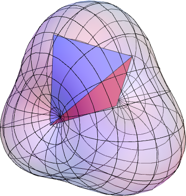
There is a general type of problem of finding special geometric configurations on families of manifolds. Quite often such problems seek to find some kind of polyhedron or polytope inscribed in a circle or sphere embedded in space. Our paper seeks to find constructible non-degenerate simplices inscribed in spheres smoothly embedded in $\mathbb{R}^{k}$. Specifically, for a given non-degenerate $k$-simplex $\Delta$, we show that among all smoothly embedded $(k-1)$ spheres in $\mathbb{R}^{k}$ isotopic to the identity through a differentiable isotopy in $\mathbb{R}^{k}$, there is a dense family of spheres such that each sphere has an inscribed simplex similar to $\Delta$ corresponding to each $U\in\operatorname{O}(k)$. An example of an embedded 2-sphere in $\mathbb{R}^{3}$ with an inscribed equilateral tetrahedra is found in Figure 1. We in fact prove more: If we let $\Sim(\Delta)$ denote the configuration space of simplices in $\mathbb{R}^{k}$ similar to a non-degenerate $k$-simplex $\Delta$, then in $\Sim(\Delta)$, the top homology class of the inscribed simplices similar to $\Delta$ on an embedded sphere maps to the top class in $\operatorname{O}(k)$.

In 1969, M.L. Gromov [16] showed that every $C^{1}$-smooth embedding of a $(k-1)$-sphere in $\mathbb{R}^{k}$ contains an inscribed simplex similar to $\Delta$ for each pose $U\in\operatorname{O}(k)$. Our results go further than Gromov. We show that the inscribed simplices in embedded spheres form a manifold cobordant to $\operatorname{O}(k)$ using configuration spaces and transversality as in [9].

Another closely related result is the 2009 work of P.V.M. Blagojević and G. Ziegler [6]. They prove that for every injective continuous maps of $f\colon\!S^{2}\rightarrow\mathbb{R}^{3}$, there are four distinct points in the image of $f$ with the property that two opposite edges have the same length and the other four edges are also of equal length. While this result holds for injective maps, our theorem recovers an even more general result for generic smooth embeddings. In addition, B. Matschke [31] proved that any smoothly embedded compact surface $S$ inscribes a particular type of tetrahedron.

All of these theorems generalize the classical results on inscribing families of triangles in planar and spatial curves. In 1978, M.D. Meyerson [34] proved that for a fixed arbitrary triangle, every simple closed curve in the plane contains the vertices of a triangle similar to the given one. He also proved that for every simple closed curve $\gamma$ in the plane, then for all, except perhaps two, points $x$ on $\gamma$, we can find points $y$ and $z$ in $\gamma$ such that $xyz$ is an equilateral triangle. In 1992, M.J. Nielsen [35] proved that for any triangle $T$ and any simple closed curve $\gamma$ in the plane, there are infinitely many triangles similar to $T$ inscribed in $\gamma$. In fact, he proves that the set of vertices corresponding to the vertex of smallest angle in $T$ is dense in $\gamma$. In 2011, Matschke [31] proved a more general result. He looked at $n$-gons whose edgelengths are in a prescribed ratio. He showed such polygons are inscribed in generic $C^{\infty}$-smooth embeddings of $S^{1}$ into a (complete) Riemannian manifold, and moreover there is a 1-parameter family of such polygons. He proves that there are an odd number of loops of such polygons that wind an odd number of times around the embedded $S^{1}$. Our main theorem and Matschke’s results are very similar for triangles inscribed in embedded curves in the plane, except that we prove (Corollary 28) that the degree of the map is 1. In 2021, A. Gupta and S. Rubinstein-Salzedo [18] generalized Nielsen’s result to any Jordan curve embedded in $\mathbb{R}^{n}$ for a restricted set of triangles dependent on certain geometric conditions. They then get a wider class of inscribed triangles by adding in regularity conditions. Namely, they show that if the curve is differentiable at a point, then any triangle can be inscribed at that point.

We pause to note that many of the inscribed triangle results were inspired by the square-peg problem: finding four points on any Jordan curve (a simple closed curve in the plane) which are the vertices of a square. This question was posed by O. Toeplitz in 1911 [44], and progress on this problem has chiefly been extension of the regularity class of simple closed curves for which the square can be found. The interested reader can find numerous articles [10, 26, 32, 36, 42] summarizing the problem, and describing the classes of curves for which the square-peg problem has been proved. There have also been many papers [1, 3, 15, 23, 22, 28, 33, 39, 45] examining quadrilaterals and polygons inscribed in curves and, more recently, making progress towards solving the rectangular-peg problem (finding rectangles of any aspect ratio inscribed in Jordan curves).

There are yet more results about inscribed and circumscribed polyhedra in spheres. For example, S. Kakutani’s theorem [24] that a compact convex body in $\mathbb{R}^{3}$ has a circumscribed cube, that is, a cube each of whose faces touch the convex body. As Matschke [32] notes, most smooth embeddings $S^{k-1}\hookrightarrow\mathbb{R}^{k}$ do not inscribe a $k$-cube for $k\geq 3$. (Intuitively, the number of equations to fulfill is larger than the degrees of freedom.) Instead asking whether crosspolytopes¹¹ 1 The regular $k$-dimensional polytope is the convex hull of $\{\pm e_{i}\}$ where $e_{i}$ are the standard basis vectors in $\mathbb{R}^{k}$. are inscribed in such an embedding might be a better generalization of inscribing a square. V.V. Makeev [30] proved the $k=3$ case, and R.N. Karasev [25] generalized the proof to arbitrary odd prime powers. Later, A. Akoypan and Karasev [2] used a limit argument to show that a simple convex polytope admits an inscribed regular octahedron. In addition, there is the work of G. Kuperberg [27] and Makeev [29] on inscribed and circumscribed polyhedra in convex bodies and spheres.

The inscribed simplex problem can be framed in terms of compactified configuration spaces. We give a short overview of the basics about these spaces in Section 2. We consider the compactified configuration space $C_{k+1}[\mathbb{R}^{k}]$ of ordered $(k+1)$-tuples of points in $\mathbb{R}^{k}$ as a manifold-with-boundary (and corners). The existence of inscribed simplices in embedded spheres can be viewed as finding the intersection of two submanifolds of $C_{k+1}[\mathbb{R}^{k}]$. The first is the submanifold of $(k+1)$-tuples of points on a $C^{\infty}$-smooth embedding $\gamma\colon\!S^{k-1}\hookrightarrow\mathbb{R}^{k}$ of a $(k-1)$-sphere in $\mathbb{R}^{k}$; the second is the submanifold of simplices in $\mathbb{R}^{k}$ which are similar to a given simplex $\Delta$, denoted by $\Sim(\Delta)$.

Theorems about intersections of manifolds are often proved by transversality arguments. There are many examples in the literature [17, 37, 43]. In [9], we provide a framework for this kind of argument adapted to configuration spaces, which we will use again in this paper. Section 3 gives a description of this method and we give a very quick overview here. We consider a smooth embedding $\gamma\colon\!S^{l}\hookrightarrow\mathbb{R}^{k}$ of $S^{l}$ in $\mathbb{R}^{k}$ Then, in the compactified configuration space $C_{n}[\mathbb{R}^{k}]$ of $n$ points in $\mathbb{R}^{k}$, we consider $C_{n}[\gamma(S^{l})]$, the compactified configuration space of $n$ points on $\gamma(S^{l})$; and $Z$ the subspace of tuples of $n$ points in $\mathbb{R}^{k}$ that satisfy the conditions of a special configuration. Now, suppose there is a different, well known, smooth embedding $i\colon\!S^{l}\hookrightarrow\mathbb{R}^{k}$ of $S^{l}$ in $\mathbb{R}^{k}$, and assume that the configuration space $C_{n}[i(S^{l})]$ is transverse to $Z$ in $C_{n}[\mathbb{R}^{k}]$. We can use Haefliger’s theorem [19] to find a differentiable isotopy between $i(S^{l})$ and $\gamma(S^{l})$ (the differentiable isotopy may need to go through $\mathbb{R}^{K}$ for $K\geq k$). The key idea is that we ought to be able to vary $C_{n}[i(S^{l})]$ to $C_{n}[\gamma(S^{l})]$ while maintaining the transversality of the intersection with $Z$. To do so, we need to make several assumptions about $Z$ and $C_{n}[\gamma(S^{l})]$ (see Section 3), and to use technical tools like multijet transversality. In the end, we are able to deduce that there is, for all $m$, a $C^{m}$-dense²² 2 The density is with respect to the Whitney $C^{\infty}$-topology, described in Section 3. set of smooth embeddings $\gamma^{\prime}\colon\!S^{l}\hookrightarrow\mathbb{R}^{k}$, such that the corresponding embeddings $C_{n}[\gamma^{\prime}]$ on configuration spaces are $C^{0}$-close to $C_{n}[\gamma]$, and that $C_{n}[\gamma^{\prime}(S^{l})]$ is transverse to $Z$, and moreover $C_{n}[i(S^{l})]\cap Z$ and $C_{n}[\gamma^{\prime}(S^{l})]\cap Z$ represent the same homology class in $Z$. We apply this method to the inscribed simplices problem in the final two sections of the paper.

In Section 4, we first describe a non-degenerate simplex in terms of the distances between distinct vertices. We then use the Cayley-Menger determinant (see Theorem 14) to give a description of when it is possible to construct a simplex from a set of distances. Secondly, we change our perspective and view a simplex $\Delta$ in $\mathbb{R}^{k}$ as an ordered $(k+1)$-tuple of distinct points in the configuration space $C_{k+1}(\mathbb{R}^{k})$. We then define $\Sim(\Delta)$ to be the space of simplices similar to $\Delta$ (through a translation, rotation, or nonzero scaling of $\mathbb{R}^{k}$). In Theorems 20 and 21 we prove that $\Sim(\Delta)$ is a submanifold of $C_{k+1}[\mathbb{R}^{k}]$ diffeomorphic to $\operatorname{O}(k)\times[0,\infty)\times\mathbb{R}^{k}$.

In Section 5 we apply our method from Section 3. Given a $C^{\infty}$-smooth embedding $\gamma\colon\!S^{k-1}\hookrightarrow\mathbb{R}^{k}$ of $S^{k-1}$ in $\mathbb{R}^{k}$, we let $C_{k+1}[\gamma(S^{k-1})]$ be the submanifold of $C_{k+1}[\mathbb{R}^{k}]$ corresponding to $(k+1)$-tuples of points on the embedded sphere $\gamma(S^{k-1})$. In Proposition 23, we show that $\Sim(\Delta)$ and $C_{k+1}[\gamma(S^{k-1}]$ are boundary disjoint in $C_{k+1}[\mathbb{R}^{k}]$. We then restrict our attention to the standard embedding of $S^{k-1}$ in $\mathbb{R}^{k}$, with corresponding configuration space $C_{k+1}[S^{k-1}]$. In Proposition 24, we show that $\Sim(\Delta)$ intersects $C_{k+1}[S^{k-1}]$ transversally and the intersection $\Sim(\Delta)\cap C_{k+1}[S^{k-1}]$ is diffeomorphic to $\operatorname{O}(k)$. Since $\operatorname{O}(k)$ is disconnected, we restrict our attention to $\Sim^{+}(\Delta)$ which is the submanifold diffeomorphic to $\operatorname{SO}(k)\times[0,\infty)\times\mathbb{R}^{k}$. We then show in Proposition 25 that the top class in $\Sim^{+}(\Delta)$ corresponds to the top homology class of $\operatorname{SO}(k)$ which also corresponds to the top class of the intersection $\Sim^{+}(\Delta)\cap C_{k+1}[S^{k-1}]$. Finally in Theorem 26, we prove there is a dense set of smooth embeddings of $S^{k-1}$ in $\mathbb{R}^{k}$ which are isotopic to the identity through a differentiable isotopy in $\mathbb{R}^{k}$, such that the subset of $\Sim^{+}(\Delta)$ of simplices inscribed in each sphere contains a similar simplex corresponding to each $U\in\operatorname{SO}(k)$. While we chose to restrict our attention to $\Sim^{+}(\Delta)$, the same results hold for $\Sim^{-}(\Delta):=\Sim(\Delta)\setminus\Sim^{+}(\Delta)$. In the special case of a smooth embedding of a circle in the plane, our results show that there are loops of triangles inscribed on an embedded circle $C^{0}$-close to the given embedding. (See Corollary 28 for a precise statement.)

The compactified configuration space of $k+1$ points in $\mathbb{R}^{k}$ is the natural setting for finding inscribed simplices in embedded spheres. In this section we give a very brief overview of compactified configuration spaces. There are many versions of this classical material (see for instance [13, 4]), but we follow D. Sinha [40] as this approach is more appropriate to our work. A discussion similar to the one found below is found in [9].

A reader familiar with configuration spaces may skip much of this section. However we recommend paying attention to the notation we have used for the spaces. Definitions 2, 3, 9, Remark 5 and Theorem 7 are particularly useful.

The space $C_{n}(M)$ is an open submanifold of $M^{\times n}$. We next compactify $C_{n}(M)$ to a closed manifold-with-boundary and corners, which we will denote $C_{n}[M]$, without changing its homotopy type. The resulting manifold will be homeomorphic to $M^{\times n}$ with an open neighborhood of the fat diagonal removed. Recall that the fat diagonal is the subset of $M^{\times n}$ of $n$-tuples for which (at least) two entries are equal, that is, where some collection of points comes together at a single point. The construction of $C_{n}[M]$ preserves information about the directions and relative rates of approach of each group of collapsing points.

We then compactify $C_{n}(\mathbb{R}^{k})$ as follows:

We now summarize some of the important features of this construction, including the fact that $C_{n}[M]$ does not depend on the choice of embedding of $M$ in $\mathbb{R}^{k}$.

The space $C_{n}[M]$ may be viewed as a polytope with a combinatorial structure based on the different ways groups of points in $M$ can come together. This structure defines a stratification of $C_{n}[M]$ into a collection of closed faces of various dimensions whose intersections are members of the collection. Full details can be found in [8, 40]. The main structure we will consider is the $(0,1,\dots,k)$-face of $\partial C_{n}[M]$. This is the boundary component where all the points come together at the same time.

Any pair $\mathbf{p}$, $\mathbf{q}$ of disjoint points in $\mathbb{R}^{k}$ has a direction $(\mathbf{p}-\mathbf{q})/\left|\mathbf{p}-\mathbf{q}\right|$ associated to it, while every triple of disjoint points $\mathbf{p}$, $\mathbf{q}$, $\mathbf{r}$ has a corresponding distance ratio $\left|\mathbf{p}-\mathbf{q}\right|/\left|\mathbf{p}-\mathbf{r}\right|$. One way to think of the coordinates of $C_{n}[M]$ is that they extend the definition of these directions and ratios to the boundary.

It turns out that for connected manifolds of dimension at least $2$, the combinatorial structure of the strata of $C_{n}[M]$ depends only on the number of points. Regardless of dimension, this construction and division of $\partial C_{n}[M]$ into strata is functorial in the following sense.

For an embedding $f\colon M\hookrightarrow N$, the image of the induced embedding $C_{n}[f]\colon C_{n}[M]\hookrightarrow C_{n}[N]$ will be denoted by $C_{n}[f(M)]$.

Finally, we will need a metric on the set of evaluation maps $C_{n}[f]\colon\!C_{n}[M]\hookrightarrow C_{n}[N]$. The definition of compactified configuration spaces allows us to view $C_{n}[N]\subset(\mathbb{R}^{k})^{n}\times(S^{k-1})^{n(n-1)}\times[0,\infty]^{n(n-1)(n-2)}$ as a metric space with the sup norm. If we define the mapping $\mbox{\rm pr}_{i}$ to be the projection onto the $i$th space of the product, then this naturally leads to a metric on the set of continuous functions $C^{0}(C_{n}[M],C_{n}[N])$.

In this section we set up a general method for tackling problems where we seek a special configuration of $n$ points on a compact manifold $M$ that is smoothly embedded in $\mathbb{R}^{k}$ (cf. [9]). In both the square-peg problem and the inscribed simplex problem, $M$ is a sphere (either $S^{1}$ or $S^{k-1}$). We thus denote the $C^{\infty}$ smooth embedding by $\gamma\colon\!S^{l}\hookrightarrow\mathbb{R}^{k}$, and the corresponding compactified configuration space of $n$ points on $\gamma(S^{l})$ is $C_{n}[\gamma(S^{l})]$. We let $Z$ denote the subspace of tuples of $n$ points in $\mathbb{R}^{k}$ that satisfy the conditions of a special configuration. For example, in [9], $Z$ is the set of all square-like quadrilaterals in $\mathbb{R}^{k}$. In this paper we are interested in $Z=\Sim(\Delta)$ (see Section 4), which is the set of all $(k+1)$-simplices in $\mathbb{R}^{k}$ which are similar to a given non-degenerate simplex $\Delta$.

The central idea is as follows: suppose there is a different, well understood, smooth embedding of $S^{l}$ in $\mathbb{R}^{k}$ (via $i\colon\!S^{l}\hookrightarrow\mathbb{R}^{k}$), and assume that the corresponding configuration space $C_{n}[i(S^{l})]$ is transverse to $Z$ in $C_{n}[\mathbb{R}^{k}]$. Also assume that $i(S^{l})$ is smoothly homotopy equivalent to $\gamma(S^{l})$ in $\mathbb{R}^{k}$. Standard transversality arguments should allow us to vary $C_{n}[i(S^{l})]$ to $C_{n}[\gamma(S^{l})]$ while maintaining the transversality of the intersection with $Z$. There are various technical obstacles to overcome, all of which are handled in detail in [9]. Here are the key steps.

Step 1: It is possible that special configurations on $\gamma(S^{l})$ shrink away to the boundary of $C_{n}[\mathbb{R}^{k}]$ during the isotopy. To prevent this, we first prove

1. (a)

   that $n$-tuples of points in $\mathbb{R}^{k}$ satisfying the geometric condition, $Z$, are a submanifold in $C_{n}(\mathbb{R}^{k})$, and that $\partial Z\subset\partial C_{n}[\mathbb{R}^{k}]$;

2. (b)

   that $C_{n}[\gamma(S^{l})]$ and $Z$ are boundary-disjoint.

For $Z=\Sim(\Delta)$, we prove 1(a) in Theorems 20 and 21. We prove 1(b) in Proposition 23.

Step 2: For a standard embedding $i\colon\!S^{l}\hookrightarrow\mathbb{R}^{k}$, we need to do two things

1. (a)

   Prove that the intersection between $C_{n}[i(S^{l})]$ and $Z$ is non-empty and transverse (in other words, $C_{n}[i]\pitchfork Z$).

2. (b)

   Compute the homology class of the intersection $C_{n}[i(S^{l})]\cap Z$ in $Z$.

For our inscribed simplex problem, we use the standard embedding $\id\colon\!S^{k-1}\hookrightarrow\mathbb{R}^{k}$ of $S^{k-1}$ in $\mathbb{R}^{k}$. We prove 2(a) in Proposition 24 and 2(b) in Proposition 25.

Step 3: Note that in order to apply our transversality arguments, we need to be able to perturb $C_{n}[\gamma(S^{l})]$ so the intersection of $Z$ remains transverse. However, there is no guarantee that the perturbed submanifold consists of configurations on a perturbed smooth embedding of $S^{l}$ in $\mathbb{R}^{k}$. We deal with this issue by applying the multijet transversality theorem [14, Theorem II.4.13]. This allows us to conclude (see [9] Theorem 17) that for any $\epsilon>0$, there is a $C^{\infty}$-open neighborhood of $\gamma$ in which there is, for all $m$, a $C^{m}$-dense set of smooth embeddings $\gamma^{\prime}\colon\!S^{l}\hookrightarrow\mathbb{R}^{k}$, such that $\|C_{n}[\gamma^{\prime}]-C_{n}[\gamma]\|_{0}<\epsilon$, and $C_{n}[\gamma^{\prime}]\pitchfork Z$, and for which $\partial Z$ and $\partial C_{n}[\gamma^{\prime}(S^{l})]$ are disjoint in $\partial C_{n}[\mathbb{R}^{k}]$.

In order to fully appreciate Step 3, first recall that the metric on the set $C^{0}(C_{n}[S^{l}],C_{n}[\mathbb{R}^{k}])$ was given in Definition 9. Second, to understand the statement about density, we need to give the topology of the spaces we are working in. In general, for manifolds $M(=S^{l})$ and $N(=\mathbb{R}^{k})$, the space $C^{\infty}(M,N)$ has the Whitney $C^{\infty}$-topology (see for instance [20]). The sets of the form

give a subbasis for the Whitney $C^{t}$-topology on $C^{t}(M,N)$ (where $t$ is finite). This subbasis is the subset of functions $g\colon M\to N$ that are smooth, and for coordinate charts $\phi\colon(U^{\prime}\subset M)\to(U\subset\mathbb{R}^{m})$ and $\psi\colon(V^{\prime}\subset N)\to(V\subset\mathbb{R}^{k})$ and $K\subset U$ compact with $g(\phi(K))\subset V^{\prime}$, then we have, for all $s\leq r$, and all $x\in\phi(K)$,

Here, $D^{s}F$ for a function $F\colon(U\subset\mathbb{R}^{m})\to(V\subset\mathbb{R}^{k})$ is the $k$-tuple of the $s$th homogeneous parts of the Taylor series representations of the projections of $F$. Finally, the subspace $C^{\infty}(M,N)$ has the Whitney $C^{\infty}$-topology by taking the union of all subbases for all $t\geq 0$.

Note that Step 3 can be applied immediately to the inscribed simplex problem.

Step 4: We need to deform standard spheres into spheres of interest and then consider what happens on the level of configuration spaces. We know precisely when such a deformation of spheres exists due to a result of A. Haefliger (which we have stated in a form useful to us).

We use Theorem 10 to find a smooth map $E\colon\!S^{l}\times I\rightarrow\mathbb{R}^{K}$ with $E(-,0)=i$ our standard embedding and $E(-,1)=\gamma^{\prime}$ (where $K$ may be greater than our original $k$). Recalling that both $C_{n}[i]$ and $C_{n}[\gamma^{\prime}]$ are transverse to $Z$ allows us to conclude that using functorality, we get a homotopy $H\colon\!C_{n}(S^{l})\times I\rightarrow C_{n}(\mathbb{R}^{K})$ with $H(-,0)=C_{n}[i]$ and $H(-,1)=C_{n}[\gamma^{\prime}]$. In [9], we then use the Transversality Homotopy Extension Theorem (see [17]), to find a map $H^{\prime}$ homotopic to $H$ and with $H^{\prime}(-,0)=H(-,0)$, $H^{\prime}(-,1)=H(-,1)$, and $H^{\prime}$ is transverse to $Z$. This then implies that in $Z$, the intersections $C_{n}[i(S^{l})]\cap Z$ and $C_{n}[\gamma^{\prime}(S^{l})]\cap Z$ represent the same homology class. In other words we have sketched a proof of the following:

In this paper we will not be making full use of Haefliger’s Theorem in Step 4. Instead, we will restrict our attention to smooth embeddings of $S^{k-1}$ in $\mathbb{R}^{k}$ which are differentiably isotopic to the identity through a differentiable isotopy in $\mathbb{R}^{k}$. The conclusion of Theorem 11 still holds for such embeddings. Putting all of our steps together allows us to conclude the following theorem.

Intuitively, this theorem shows that any smooth embedding $\gamma$ of $S^{l}$ in $\mathbb{R}^{k}$ has a neighborhood in which there is a dense set of smooth embeddings $\gamma^{\prime}$ for which $C_{n}[\gamma^{\prime}(S^{l})]$ is guaranteed to have certain intersections with various submanifolds of $C_{n}[\mathbb{R}^{k}]$ defined by geometric conditions. Stated in a different way, we have the idea that a dense set of embeddings of $S^{l}$ always contain certain inscribed configurations of points.

References

- [1] Arseniy Akopyan and Sergey Avvakumov. Any cyclic quadrilateral can be inscribed in any closed convex smooth curve. Forum Math. Sigma, 6:Paper No. e7, 9, 2018.
- [2] Arseniy Akopyan and Roman Karasev. Inscribing a regular octahedron into polytopes. Discrete Math., 313(1):122–128, 2013.
- [3] Jai Aslam, Shujian Chen, Florian Frick, Sam Saloff-Coste, Linus Setiabrata, and Hugh Thomas. Splitting loops and necklaces: variants of the square peg problem. Forum Math. Sigma, 8:Paper No. e5, 16, 2020.
- [4] Scott Axelrod and Isadore M. Singer. Chern-Simons perturbation theory. II. J. Differential Geom., 39(1):173–213, 1994.
- [5] Marcel Berger. Geometry. I. Universitext. Springer-Verlag, Berlin, 1987. Translated from the French by M. Cole and S. Levy.
- [6] Pavle V. M. Blagojević and Günter M. Ziegler. Tetrahedra on deformed spheres and integral group cohomology. Electron. J. Combin., 16(2):Research Paper 16, 11, 2009. Special volume in honor of Anders Björner.
- [7] Leonard M. Blumenthal and Basil E. Gillam. Distribution of points in -space. Amer. Math. Monthly, 50:181–185, 1943.
- [8] Ryan Budney, James Conant, Kevin P. Scannell, and Dev P. Sinha. New perspectives on self-linking. Adv. Math., 191(1):78–113, 2005.
- [9] Jason Cantarella, Elizabeth Denne, and John McCleary. Configuration spaces, multijet transversality, and the square-peg problem, arXiv:2103.07506. 2021.
- [10] Jason Cantarella, Elizabeth Denne, and John McCleary. Square-like quadrilaterals inscribed in embedded space curves, arXiv:2103.13848. 2021.
- [11] Harold S.M. Coxeter. The Circumradius of the General Simplex. Math. Gaz., 15(210):229–231, 1930.
- [12] Luca Dieci and Timo Eirola. On smooth decompositions of matrices. SIAM J. Matrix Anal. Appl., 20(3):800–819, 1999.
- [13] William Fulton and Robert MacPherson. A compactification of configuration spaces. Ann. of Math. (2), 139(1):183–225, 1994.
- [14] Martin Golubitsky and Victor Guillemin. Stable mappings and their singularities. Springer-Verlag, New York, 1973. Graduate Texts in Mathematics, Vol. 14.
- [15] Joshua Evan Greene and Andrew Lobb. The rectangular peg problem. Ann. of Math. (2), 194(2):509–517, 2021.
- [16] Mikhael L. Gromov. Simplexes inscribed on a hypersurface. Mat. Zametki, 5:81–89, 1969.
- [17] Victor Guillemin and Alan Pollack. Differential topology. AMS Chelsea Publishing, Providence, RI, 2010. Reprint of the 1974 original.
- [18] Aryaman Gupta and Simon Rubinstein-Salzedo. Inscribed triangles of Jordan curves in , arXiv:2102.03953. 2021.
- [19] André Haefliger. Differentiable imbeddings. Bull. Amer. Math. Soc., 67:109–112, 1961.
- [20] Morris W. Hirsch. Differential topology, volume 33 of Graduate Texts in Mathematics. Springer-Verlag, New York, 1994. Corrected reprint of the 1976 original.
- [21] Roger A. Horn and Charles R. Johnson. Matrix analysis. Cambridge University Press, Cambridge, second edition, 2013.
- [22] Cole Hugelmeyer. Inscribed rectangles in a smooth Jordan curve attain at least one third of all aspect ratios. Ann. of Math. (2), 194(2):497–508, 2021.
- [23] Cole Hugelmeyer. Every smooth Jordan curve has an inscribed rectangle with aspect ratio equal to , arXiv:1803.07417. 2018.
- [24] Shizuo Kakutani. A proof that there exists a circumscribing cube around any bounded closed convex set in . Ann. of Math. (2), 43:739–741, 1942.
- [25] Roman N. Karasev. Inscribing a regular crosspolytope, arXiv:0905.2671. 2009.
- [26] Victor Klee and Stan Wagon. Old and new unsolved problems in plane geometry and number theory. The Dolciani Mathematical Expositions, 11. Mathematical Association of America, 1991.
- [27] Greg Kuperberg. Circumscribing constant-width bodies with polytopes. New York J. Math., 5:91–100, 1999.
- [28] V. V. Makeev. On quadrangles inscribed in a closed curve and the vertices of the curve. Zap. Nauchn. Sem. S.-Peterburg. Otdel. Mat. Inst. Steklov. (POMI), 299(Geom. i Topol. 8):241–251, 331, 2003.
- [29] V. V. Makeev. Inscribed and circumscribed polyhedra for a convex body and a problem on continuous functions on a sphere in Euclidean space. Algebra i Analiz, 18(6):187–204, 2006.
- [30] V.V. Makeev. Universally inscribed and outscribed polytopes. PhD thesis, St. Petersburg State University, 2003.
- [31] Benjamin Matschke. Equivariant topology methods in discrete geometry. PhD thesis, Freie Universität, 2011.
- [32] Benjamin Matschke. A survey on the square peg problem. Notices Amer. Math. Soc., 61(4):346–352, 2014.
- [33] Benjamin Matschke. Quadrilaterals inscribed in convex curves. Trans. Amer. Math. Soc., 374(8):5719–5738, 2021.
- [34] Mark D. Meyerson. Equilateral triangles and continuous curves. Fund. Math., 110(1):1–9, 1980.
- [35] Mark J. Nielsen. Triangles inscribed in simple closed curves. Geom. Dedicata, 43(3):291–297, 1992.
- [36] Igor Pak. Lectures on Discrete and Polyhedral Geometry. Free online text. 2010.
- [37] Hans Samelson. Note on vector fields in manifolds. Proc. Amer. Math. Soc., 36:272–274, 1972.
- [38] Issac J. Schoenberg. Remarks to Maurice Fréchet’s article “Sur la définition axiomatique d’une classe d’espace distanciés vectoriellement applicable sur l’espace de Hilbert”. Ann. of Math. (2), 36(3):724–732, 1935.
- [39] Richard Evan Schwartz. A trichotomy for rectangles inscribed in Jordan loops. Geom. Dedicata, 208:177–196, 2020.
- [40] Dev P. Sinha. Manifold-theoretic compactifications of configuration spaces. Selecta Math. (N.S.), 10(3):391–428, 2004.
- [41] Manfred J. Sippl and Harold A. Scheraga. Cayley-Menger coordinates. Proc. Nat. Acad. Sci. U.S.A., 83(8):2283–2287, 1986.
- [42] Terence Tao. An integration approach to the Toeplitz square peg problem. Forum Math. Sigma, 5:Paper No. e30, 63, 2017.
- [43] René Thom. Quelques propriétés globales des variétés différentiables. Comment. Math. Helv., 28:17–86, 1954.
- [44] Otto Toeplitz. Ueber einige aufgaben der analysis situs. Verhandlugen Der Schwizerischen Naturafoschenden Gesellshaft in Solothurn, 4:197, 1922.
- [45] Siniša T. Vrećica and Rade T. Živaljević. Fulton-MacPherson compactification, cyclohedra, and the polygonal pegs problem. Israel J. Math., 184:221–249, 2011.
Appendix A Results from Linear Algebra
We will let denote the set of all matrices, and let denote the set of all matrices. Recall that a symmetric matrix is a square matrix that is equal to its transpose: . That is, is symmetric if and only if . Also recall that
- •
An symmetric real matrix is positive-definite if for all .
An symmetric real matrix is positive semidefinite of non-negative-definite if for all .
Similar definitions hold for negative-definite and negative semidefinite.
We now review some theorems about symmetric matrices.
Theorem 29 (See [21] Theorem 7.2.6).
Let be an symmetric and positive semidefinite matrix, let , and let . Then there is a unique symmetric positive semidefinite matrix such that .
Remark 30.
While this theorem only guarantees a unique positive semidefinite square root for a semidefinite matrix , an examination of the proof in [21] shows that more has been proven. The proof shows there is a unique positive definite square root for a positive definite matrix .
Theorem 31 (See [21] Theorem 7.2.7).
Let be an symmetric matrix. If , with an matrix, then is positive definite if and only if has full column rank.
The polar decomposition of a matrix is incredibly useful. Below, we give the version that best applies to our work.
Theorem 32 (See [21] Theorem 7.3.1 Polar decomposition).
Let be an real matrix. Then , in which are positive semidefinite and is orthogonal. The factors and are uniquely determined; is a polynomial in and is a polynomial in . The factor is uniquely determined if is nonsingular.
Remark 33 (See [12] Section 2.3 (c)).
Suppose is an matrix with full rank and depends -smoothly on . Then we can write , where is orthonormal, is symmetric positive definite and and are as smooth as .