August 11, 2026

Current bounds on the Type-Z $Z_{3}$ three Higgs doublet modelPreprint: CFTP/21-010

Rafael Boto Email: rafael.boto@tecnico.ulisboa.pt Affiliation: Departamento de Física and CFTP, Instituto Superior Técnico
Universidade de Lisboa, Av. Rovisco Pais 1, 1049-001 Lisboa, Portugal Jorge C. Romão Email: jorge.romao@tecnico.ulisboa.pt Affiliation: Departamento de Física and CFTP, Instituto Superior Técnico
Universidade de Lisboa, Av. Rovisco Pais 1, 1049-001 Lisboa, Portugal João P. Silva Email: jpsilva@cftp.ist.utl.pt Affiliation: Departamento de Física and CFTP, Instituto Superior Técnico
Universidade de Lisboa, Av. Rovisco Pais 1, 1049-001 Lisboa, Portugal

Abstract

Type-Z models, where charged leptons, up type quarks and down type quarks each couple to a different scalar, are only possible when there are three or more Higgs doublets. We consider the Type-Z three Higgs doublet model imposed by a softly broken $\mathbbm{Z}_{3}$ symmetry. We take into account all theoretical and experimental constraints, including perturbative unitarity and bounded from below conditions that we develop here. Since there can be cancellations between the two charged Higgs in $B\rightarrow X_{s}\gamma$ (and in $h\rightarrow\gamma\gamma$ ), the lower bounds obtained on the charged Higgs masses are alleviated. We also discuss in detail the important physical differences between exact alignment and approximate alignment, and present some useful benchmark points.

pacs

14.60.Pq 12.60.Fr 14.60.St

After the observation in 2012 by ATLAS and CMS Aad:2012tfa; Chatrchyan:2012ufa of a new scalar particle closely resembling the Standard Model (SM) Higgs boson, the search for physics beyond the Standard Model (BSM) is now the main goal of the LHC experiments. Popular extensions where only Higgs doublets are added to the SM have been extensively studied and allow for both the agreement with the experimental results and the possibility of new features; for reviews see Gunion:1989we; Branco:2011iw; Ivanov:2017dad.

The simplest extension, the two-Higgs-doublet model (2HDM), can provide new sources of CP-violation necessary to fulfill the Sakharov criteria for baryogenesis Sakharov:1967dj. However, the most general Higgs-fermion Yukawa couplings generically yield Higgs-mediated flavor-changing neutral “currents” (FCNCs) at tree level, in conflict with experimental observations. A common method to have FCNCs sufficiently suppressed is to impose symmetries on the Lagrangian: tree-level FCNC effects can be completely removed by establishing how the fermion and scalar fields have to transform under the chosen symmetry. In the two Higgs doublet model (2HDM) this can be achieved by imposing a $\mathbbm{Z}_{2}$ symmetry Glashow:1976nt; Paschos:1976ay. Reference Ferreira:2010xe showed that in general N Higgs doublet models (NHDM) the Yukawa coupling matrices to fermions of a given electric charge remain proportional (thus removing FCNCs) under the renormalization group running if and only if there is a basis for the Higgs doublets in which all the fermions of a given electric charge couple to only one Higgs doublet. The models are then classified based on these choices. The four (five) distinct types of Yukawa couplings in models with two (more than two) doublets that fit this requirement were introduced in Ferreira:2010xe and denoted in Yagyu:2016whx by Types I, II, X (also known as lepton-specific), Y (flipped), and Z, according to

Type-I:	$\displaystyle\phi_{u}=\phi_{d}=\phi_{e}\,,$
Type-II:	$\displaystyle\phi_{u}\neq\phi_{d}=\phi_{e}\,,$
Type-X:	$\displaystyle\phi_{u}=\phi_{d}\neq\phi_{e}\,,$
Type-Y:	$\displaystyle\phi_{u}=\phi_{e}\neq\phi_{d}\,,$
Type-Z:	$\displaystyle\phi_{u}\neq\phi_{d};\ \phi_{d}\neq\phi_{e},\ \phi_{e}\neq\phi_{u}\,,$	(1)

where $\phi_{u,d,e}$ are the single scalar fields that couple exclusively to the up type quarks, down type quarks, and charged leptons, respectively. In this work, we set our attention on the Type-Z that can only appear for NHDM with $N>2$ . It is interesting to see what differences there are in this new type of model, since it decouples completely the up quark, down quark and charged lepton sectors from one-another.

There are have been implementations of Type-Z in three-Higgs-doublet models (3HDM) using a $\mathbbm{Z}_{2}\times\mathbbm{Z}_{2}$ symmetry Akeroyd:2020nfj; Logan:2020mdz or $\mathbbm{Z}_{3}$ Das:2019yad; Boto:2021. For this work, we choose to use a $\mathbbm{Z}_{3}$ symmetric potential. This symmetry is realizable through the following representation,

S_{\mathbbm{Z}_{3}}=\text{diag}(1,e^{i\frac{2\pi}{3}}e^{-i\frac{2\pi}{3}}).

(2)

Recently, there has been an analysis of $\mathbbm{Z}_{3}$ 3HDM which takes the exact alignment limit and looks at specific values of the physical parameters Chakraborti:2021bpy. It does not seem to consider the theoretical constraints coming from perturbative unitarity, discussed explicitly for the $\mathbbm{Z}_{3}$ 3HDM model in Ref. Bento:2017eti and BFB conditions, which we develop here. Compatibility with the bounds coming from Higgs searches is also checked with the newest version of the HiggsBounds-5.9.1 (HB5) code Bechtle:2020pkv. In particular, we show that recent LHC measurements exclude all points in Fig. 2 of Ref. Chakraborti:2021bpy, for the same parameter choices. We then show that by scanning for a larger range of parameters (away from exact alignment, but still consistent with all experimental data) we can obtain viable points corresponding to smaller masses for the additional particles.

In Sec. I we describe succinctly the scalar and Yukawa sectors of the $\mathbbm{Z}_{3}$ 3HDM model, discussed also in Das:2019yad; Boto:2021; Chakraborti:2021bpy. The theoretical and experimental constraints are described in Sec. II. In Sec. III we describe the impact of current LHC measurements on the 125GeV scalar decays, both excluding and including the impact of HB5 bounds. In particular, we discuss the fact that the couplings of the two charged scalars may have different signs, thus allowing for canceling contributions to $h\rightarrow\gamma\gamma$ . A similar effect is possible in $B\to X_{s}\gamma$ , thus alleviating the lower bounds on charged scalar masses. This is discussed in Sec. IV and Sec. V, where we explore the regions of parameters allowed by the different constraints imposed, starting from the experimental limits on the BR( $B\to X_{s}\gamma$ ) and progressively varying the ranges on our parameter scans. Our work highlights the importance of going beyond strict alignment, when procuring the full range of possibilities existent within the $\mathbbm{Z}_{3}$ 3HDM. We present illustrative benchmark points in Sec. VII and discuss our conclusions in Sec. VIII, leaving the appendix for the full expression of some couplings required in our calculations.

I The $\mathbbm{Z}_{3}$ 3HDM Model

I.1 Scalar sector

Taking the potential defined by Das:2019yad, the terms invariant under the chosen transformation, $\phi_{i}\to\phi_{i}^{\prime}=(S_{\mathbbm{Z}_{3}})_{ij}\phi_{j}$ , are given by

V_{\mathbbm{Z}_{3}}=V_{\text{quadratic}}+V_{\text{quartic}},

(3)

with the quartic part

$\displaystyle V_{\text{quartic}}$	$\displaystyle=$	$\displaystyle\lambda_{1}(\phi_{1}^{\dagger}\phi_{1})^{2}+\lambda_{2}(\phi_{2}^{\dagger}\phi_{2})^{2}+\lambda_{3}(\phi_{3}^{\dagger}\phi_{3})^{2}+\lambda_{4}(\phi_{1}^{\dagger}\phi_{1})(\phi_{2}^{\dagger}\phi_{2})+\lambda_{5}(\phi_{1}^{\dagger}\phi_{1})(\phi_{3}^{\dagger}\phi_{3})$	(4)
		$\displaystyle\quad+\lambda_{6}(\phi_{2}^{\dagger}\phi_{2})(\phi_{3}^{\dagger}\phi_{3})+\lambda_{7}(\phi_{1}^{\dagger}\phi_{2})(\phi_{2}^{\dagger}\phi_{1})+\lambda_{8}(\phi_{1}^{\dagger}\phi_{3})(\phi_{3}^{\dagger}\phi_{1})+\lambda_{9}(\phi_{2}^{\dagger}\phi_{3})(\phi_{3}^{\dagger}\phi_{2})$
		$\displaystyle\quad+\left[\lambda_{10}(\phi_{1}^{\dagger}\phi_{2})(\phi_{1}^{\dagger}\phi_{3})+\lambda_{11}(\phi_{1}^{\dagger}\phi_{2})(\phi_{3}^{\dagger}\phi_{2})+\lambda_{12}(\phi_{1}^{\dagger}\phi_{3})(\phi_{2}^{\dagger}\phi_{3})+\text{h.c.}\right],$

and the quadratic part

V_{\text{quadratic}}=m_{11}^{2}\phi_{1}^{\dagger}\phi_{1}+m_{22}^{2}\phi_{2}^{\dagger}\phi_{2}+m_{33}^{2}\phi_{3}^{\dagger}\phi_{3}+\left[m_{12}^{2}(\phi_{1}^{\dagger}\phi_{2})+m_{13}^{2}(\phi_{1}^{\dagger}\phi_{3})+m_{23}^{2}(\phi_{2}^{\dagger}\phi_{3})+\text{h.c.}\right],

(5)

also including terms, $m_{12}^{2}$ , $m_{13}^{2}$ and $m_{23}^{2}$ , that break the symmetry softly.

After spontaneous symmetry breaking (SSB), the three doublets can be parameterized in terms of its component fields as:¹¹ 1 Notice that we use $x_{i}$ in place of Ref. Das:2019yad’s $h_{i}$ , because for us $h_{i}$ are the physical neutral scalar mass eigenstates.

\phi_{i}=\begin{pmatrix}w_{k}^{\dagger}\\ (v_{i}+x_{i}\,+\,i\,z_{i})/\sqrt{2}\end{pmatrix}\,\,,\qquad(i=1,2,3)

(6)

where $v_{i}/\sqrt{2}$ corresponds to the vacuum expectation value (vev) for the neutral component of $\phi_{i}$ . It is assumed that the scalar sector of the model explicitly and spontaneously conserves CP.²² 2 Strictly speaking, it is not advisable to assume a real scalar sector while allowing the Yukawa couplings to carry the phase necessary for the CKM matrix. This is also a problem with the so-called real 2HDM Fontes:2021znm. One can take the view that the complex terms and their counterterms in the scalar sector exist, with the former set to zero.

That is, all the parameters in the scalar potential are real and the vevs $v_{1}$ , $v_{2}$ , $v_{3}$ , are also real. With this assumption, the scalar potential of Eq. (3) contains eighteen parameters. The vevs can be parameterized as follows:

v_{1}=v\cos\beta_{1}\cos\beta_{2}\,,\qquad v_{2}=v\sin\beta_{1}\cos\beta_{2}\,,\qquad v_{3}=v\sin\beta_{2},

(7)

leading to the Higgs basis Georgi:1978ri; Donoghue:1978cj; Botella:1994cs to be obtained by the following rotation,

\begin{pmatrix}H_{0}\\ R_{1}\\ R_{2}\end{pmatrix}=\mathcal{O}_{\beta}\begin{pmatrix}x_{1}\\ x_{2}\\ x_{3}\end{pmatrix}=\begin{pmatrix}\cos\beta_{2}\cos\beta_{1}&\cos\beta_{2}\sin\beta_{1}&\sin\beta_{2}\\ -\sin\beta_{1}&\cos\beta_{1}&0\\ -\cos\beta_{1}\sin\beta_{2}&-\sin\beta_{1}\sin\beta_{2}&\cos\beta_{2}\end{pmatrix}\begin{pmatrix}x_{1}\\ x_{2}\\ x_{3}\end{pmatrix}.

(8)

The scalar kinetic Lagrangian is written as

\mathscr{L}_{\text{kin}}=\sum_{k=1}^{n=3}|D_{\mu}\phi_{k}|^{2},

(9)

and contains the terms relevant to the propagators and trilinear couplings of the scalars and gauge bosons.

We can now define orthogonal matrices which diagonalize the squared-mass matrices present in the CP-even scalar, CP-odd scalar and charged scalar sectors. These are the transformations that take us to the physical basis, with states possessing well-defined masses. Following Ref. Das:2019yad; Boto:2021, the twelve quartic couplings can be exchanged for seven physical masses (three CP-even scalars, two CP-odd scalars and two pairs of charged scalars) and five mixing angles. The mass terms in the neutral scalar sector can be extracted through the following rotation,

\begin{pmatrix}h_{1}\\ h_{2}\\ h_{3}\end{pmatrix}=\mathcal{O}_{\alpha}\begin{pmatrix}x_{1}\\ x_{2}\\ x_{3}\end{pmatrix},

(10)

where we take $h_{1}\equiv h_{125}$ to the be the 125GeV Higgs particle found at LHC. The form chosen for $\mathcal{O}_{\alpha}$ is

\textbf{R}\equiv\mathcal{O}_{\alpha}=\mathcal{R}_{3}.\mathcal{R}_{2}.\mathcal{R}_{1},

(11)

where

\mathcal{R}_{1}=\begin{pmatrix}c_{\alpha_{1}}&s_{\alpha_{1}}&0\\ -s_{\alpha_{1}}&c_{\alpha_{1}}&0\\ 0&0&1\end{pmatrix}\,,\quad\mathcal{R}_{2}=\begin{pmatrix}c_{\alpha_{2}}&0&s_{\alpha_{2}}\\ 0&1&0\\ -s_{\alpha_{2}}&0&c_{\alpha_{2}}\end{pmatrix}\,,\quad\mathcal{R}_{3}=\begin{pmatrix}1&0&0\\ 0&c_{\alpha_{3}}&s_{\alpha_{3}}\\ 0&-s_{\alpha_{3}}&c_{\alpha_{3}}\end{pmatrix}\,.\quad

(12)

For the CP-odd scalar sector, the physical basis is chosen as $\begin{pmatrix}G^{0}&A_{1}&A_{2}\end{pmatrix}^{T}$ and the transformation to be

\begin{pmatrix}G^{0}\\ A_{1}\\ A_{2}\end{pmatrix}=\mathcal{O}_{\gamma_{1}}\mathcal{O}_{\beta}\begin{pmatrix}z_{1}\\ z_{2}\\ z_{3}\end{pmatrix},

(13)

where $\mathcal{O}_{\gamma_{1}}$ is defined in order to diagonalize the 2x2 submatrix that remains in the Higgs basis, with the form

\mathcal{O}_{\gamma_{1}}=\begin{pmatrix}1&0&0\\ 0&c_{\gamma_{1}}&-s_{\gamma_{1}}\\ 0&s_{\gamma_{1}}&c_{\gamma_{1}}\end{pmatrix}.

(14)

For later use, we define the matrix P as the combination

\textbf{P}\equiv\mathcal{O}_{\gamma_{1}}\mathcal{O}_{\beta}.

(15)

For the charged scalar sector, the physical basis is $\begin{pmatrix}G^{+}&H_{1}^{+}&H_{2}^{+}\end{pmatrix}^{T}$ and the transformation is

\begin{pmatrix}G^{+}\\ H_{1}^{+}\\ H_{2}^{+}\end{pmatrix}=\mathcal{O}_{\gamma_{2}}\mathcal{O}_{\beta}\begin{pmatrix}w_{1}^{\dagger}\\ w_{2}^{\dagger}\\ w_{3}^{\dagger}\end{pmatrix},

(16)

where

\mathcal{O}_{\gamma_{2}}=\begin{pmatrix}1&0&0\\ 0&c_{\gamma_{2}}&-s_{\gamma_{2}}\\ 0&s_{\gamma_{2}}&c_{\gamma_{2}}\end{pmatrix}.

(17)

We write the masses of $H_{1}^{+}$ and $H_{2}^{+}$ as $m_{H_{1}^{\pm}}$ and $m_{H_{2}^{\pm}}$ , respectively. The matrix Q is then defined as the combination

\textbf{Q}\equiv\mathcal{O}_{\gamma_{2}}\mathcal{O}_{\beta}.

(18)

Considering that the states in the physical basis have well-defined masses, we can obtain relations between the set

	$\displaystyle\left\{v_{1},v_{2},v_{3},m_{h1},m_{h2},m_{h3},m_{A1},m_{A2},m_{H_{1}^{\pm}},m_{H_{2}^{\pm}},\alpha_{1},\alpha_{2},\alpha_{3},\gamma_{1},\gamma_{2}\right\},$		(19)
	$\displaystyle\quad v_{1}=v\cos\beta_{1}\cos\beta_{2}\,,\quad\,v_{2}=v\sin\beta_{1}\cos\beta_{2}\,,\quad\,v_{3}=v\sin\beta_{2},$		(20)

and the parameters of the potential in Eq. (3), as shown in Ref. Das:2019yad; Boto:2021. We performed an extensive scan of the parameter space in Eq. (19). Our fixed inputs are $v=246\,\text{GeV}$ and $m_{h1}=125\,\text{GeV}$ . We then took random values in the ranges:

	$\displaystyle\alpha_{1},\,\alpha_{2},\,\alpha_{3},\,\gamma_{1},\,\gamma_{2}\,\in\left[-\frac{\pi}{2},\frac{\pi}{2}\right];\qquad\tan{\beta_{1}},\,\tan{\beta_{2}}\,\in\left[0,10\right];$
	$\displaystyle m_{h2},\,m_{h3}\,\in\left[125,1000\right]\,\text{GeV};\qquad m_{A_{1}},\,m_{A_{2}}\,m_{H_{1}^{\pm}},\,m_{H_{2}^{\pm}}\,\in\left[100,1000\right]\,\text{GeV}.$		(21)

These parameter ranges will be used in all scans and figures presented below, except where noted otherwise. The lower limits chosen for the masses satisfy the constraints listed in Ref. Aranda:2019vda.³³ 3 Ref. Aranda:2019vda has the same $\mathbbm{Z}_{3}$ 3HDM scalar sector, but it does not couple to fermions as a Type-Z model because the aim there is to have two Inert scalar doublets and only one active one.

I.2 Higgs-Fermion Yukawa interactions

One can now impose the Type-Z model on the Yukawa Lagrangian, by establishing how the fields behave under the $\mathbbm{Z}_{3}$ transformation. For this, there are multiple possibilities that differ on which of the scalars gives mass to each type of fermion. We follow the choice made by Das and Saha Das:2019yad. The scalar doublets $\phi_{1}$ and $\phi_{2}$ transform nontrivially as:

\phi_{1}\to\omega\phi_{1}\,,\qquad\phi_{2}\to\omega^{2}\phi_{2},

(22)

where $\omega=e^{2\pi\,i/3}$ . For the fermionic fields, we consider that under $\mathbbm{Z}_{3}$

d_{R}\to\omega d_{R}\,,\qquad l_{R}\to\omega^{2}\,l_{R},

(23)

while the rest of the fields remain unaffected. It follows that the Yukawa coupling matrices are now restricted: $\phi_{1}$ only has interaction terms with the charged leptons, giving them mass; $\phi_{3}$ and $\phi_{2}$ are responsible for masses of the up and down type quarks, respectively.

When taking into account the restrictions imposed by the symmetry, the Yukawa couplings to fermions can be written in a compact form. For the couplings of neutral Higgs to fermions,

\mathscr{L}_{\rm Y}\ni-\frac{m_{f}}{v}\bar{f}(a^{f}_{j}+i\,b^{f}_{j}\gamma_{5})fh_{j},

(24)

where we group the physical Higgs fields in a vector, as $h_{j}\equiv(h_{1},h_{2},h_{3},A_{1},A_{2})_{j}$ . The coefficients are given in Eq. (25),

$\displaystyle a_{j}^{f}$	$\displaystyle\to$	$\displaystyle\frac{\textbf{R}_{j,1}}{\hat{v_{1}}},\qquad\qquad j=1,2,3\qquad\text{for all leptons},$
$\displaystyle b_{j}^{f}$	$\displaystyle\to$	$\displaystyle\frac{\textbf{P}_{j-2,1}}{\hat{v_{1}}},\qquad\quad j=4,5\quad\qquad\text{for all leptons},$
$\displaystyle a_{j}^{f}$	$\displaystyle\to$	$\displaystyle\frac{\textbf{R}_{j,3}}{\hat{v_{3}}},\qquad\qquad j=1,2,3\qquad\text{for all up quarks},$
$\displaystyle b_{j}^{f}$	$\displaystyle\to$	$\displaystyle-\frac{\textbf{P}_{j-2,3}}{\hat{v_{3}}},\quad\quad j=4,5\quad\qquad\text{for all up quarks},$
$\displaystyle a_{j}^{f}$	$\displaystyle\to$	$\displaystyle\frac{\textbf{R}_{j,2}}{\hat{v_{2}}},\qquad\qquad j=1,2,3\qquad\text{for all down quarks},$
$\displaystyle b_{j}^{f}$	$\displaystyle\to$	$\displaystyle\frac{\textbf{P}_{j-2,2}}{\hat{v_{2}}},\qquad\quad j=4,5\quad\qquad\text{for all down quarks},$	(25)

where we introduce $\hat{v_{i}}=v_{i}/v$ , with the vevs in Eq. (7). Note how the coupling of each type of fermion depends on entries of the diagonalization matrices in Eqs. (11) and (15).

The couplings of the charged Higgs, $H_{1}^{\dagger}$ and $H_{2}^{\dagger}$ , to fermions can be expressed as

	$\displaystyle\mathscr{L}_{\rm Y}$	$\displaystyle\ni$	$\displaystyle\frac{\sqrt{2}}{v}\bar{\psi}_{d_{i}}\left[m_{\psi_{d_{i}}}V_{ji}^{\ast}\,\eta_{k}^{L}P_{L}+m_{\psi_{u_{j}}}V_{ji}^{\ast}\,\eta_{k}^{R}P_{R}\right]\psi_{u_{j}}H_{k}^{-}$		(26)
			$\displaystyle+\frac{\sqrt{2}}{v}\bar{\psi}_{u_{i}}\left[m_{\psi_{d_{j}}}V_{ij}\,\eta_{k}^{L}P_{R}+m_{\psi_{u_{i}}}V_{ij}\,\eta_{k}^{R}P_{L}\right]\psi_{d_{j}}H_{k}^{+},$		(26)

where $(\psi_{u_{i}},\psi_{d_{i}})$ is $(u_{i},d_{i})$ for quarks or $(\nu_{i},l_{i})$ for leptons. For quarks, $V$ is the CKM matrix, while for leptons, $V_{ij}=\delta_{ij}$ since we are considering massless neutrinos. The couplings are

\eta_{k}^{l\,L}=-\frac{\textbf{Q}_{k+1,1}}{\hat{v_{1}}}\,,\quad\eta_{k}^{l\,R}=0\,,\quad\eta_{k}^{q\,L}=-\frac{\textbf{Q}_{k+1,2}}{\hat{v_{2}}}\,,\quad\eta_{k}^{q\,R}=\frac{\textbf{Q}_{k+1,3}}{\hat{v_{3}}}\,,\quad\text{k=1,2},

(27)

for leptons and quarks, respectively.

II Constraints on the parameter space

In this section we study the constraints that must be applied to the model parameters in order to ensure consistency.

II.1 Theoretical Constraints 1

We impose perturbativity unitarity, sufficient bounded from below (BFB) conditions, and the oblique parameters $S$ , $T$ , and $U$ .

II.1.1 BFB conditions on the 3HDM

As basic requirements for any physical theory, the Higgs potential must satisfy conditions that ensure it possesses a stable minimum, around which one can perform perturbative calculations. That is, it must be bounded from below, meaning that there is no direction in field space along which the value of the potential tends to minus infinity. This need of a non-trivial minimum is then translated to conditions on the parameters of the potential.

Focusing on the study of the 3HDM constrained by a $\mathbbm{Z}_{3}$ symmetry, the quartic terms in Eq. (4) can be written as

V_{\text{quartic}}=V_{0}+V_{1},

(28)

where $V_{0}$ has the terms in $\lambda_{1\to 9}$ and $V_{1}$ the terms $\lambda_{10\to 12}$ . If the potential were just $V_{0}$ in Eq. (28), then the BFB necessary and sufficient conditions would be simply those given by Klimenko in Ref. Klimenko:1984qx. The problem, not yet solved for the 3HDM with a $\mathbbm{Z}_{3}$ symmetry is the $V_{1}$ part. We will introduce sufficient conditions for BFB by bounding the potential by a lower potential. To do that we follow Klimenko:1984qx; Fontes:2019uld, checking for neutral minima. Neutral directions in the Higgs space correspond to situations when all $\phi_{i}$ are proportional to each other⁴⁴ 4 Other directions, along which the strict proportionality of all three doublets does not hold, are called charge-breaking (CB) directions. In recent works Faro:2019vcd; Ivanov:2020jra, it has been proven that these directions can lead to pathological situations for other symmetries in the 3HDM. It is then required to consider these directions when doing a complete work of looking for necessary and sufficient BFB conditions. Our contribution to the analysis of the $\mathbbm{Z}_{3}$ symmetry is to specify sufficient conditions along the neutral direction.. Along these directions, we can then define

\phi_{1}\to\sqrt{x}e^{i\theta_{1}},\qquad\phi_{2}\to\sqrt{y}e^{i\theta_{2}},\qquad\phi_{3}\to\sqrt{z}e^{i\theta_{3}}.

(29)

It then follows that for $V_{0}$ ,

	$\displaystyle V_{0}$	$\displaystyle=$	$\displaystyle\lambda_{1}x^{2}+\lambda_{2}y^{2}+\lambda_{3}z^{2}+\lambda_{4}xy+\lambda_{5}xz+\lambda_{6}yz+\lambda_{7}xy+\lambda_{8}xz+\lambda_{9}yz$		(30)
		$\displaystyle=$	$\displaystyle\lambda_{1}x^{2}+\lambda_{2}y^{2}+\lambda_{3}z^{2}+(\lambda_{4}+\lambda_{7})xy+(\lambda_{5}+\lambda_{8})xz+(\lambda_{6}+\lambda_{9})yz,$		(30)

and for $V_{1}$ ,

V_{1}=2\lambda_{10}x\sqrt{y}\sqrt{z}\cos\delta_{1}+2\lambda_{11}y\sqrt{x}\sqrt{z}\cos\delta_{2}+2\lambda_{12}z\sqrt{x}\sqrt{y}\cos\delta_{3},

(31)

where $\delta_{i}$ are some combination of the phases $\theta_{i}$ . Considering that $x,y,z>0$ by definition, we can start our strategy of bounding the potential by a lower one with

V_{1}\geq V_{1}^{\prime}=-2|\lambda_{10}|x\sqrt{y}\sqrt{z}-2|\lambda_{11}|y\sqrt{x}\sqrt{z}-2|\lambda_{12}|z\sqrt{x}\sqrt{y}.

(32)

Notice that for non-negative $x,y,z$ one has

-\sqrt{x}\sqrt{z}>-x-y,\qquad-\sqrt{x}\sqrt{z}>-x-z,\qquad-\sqrt{y}\sqrt{z}>-y-z.

(33)

Therefore,

V_{1}\geq V_{1}^{\prime}>V_{1}^{\prime\prime}=-2|\lambda_{10}|(xy+xz)-2|\lambda_{11}|(xy+yz)-2|\lambda_{12}|(xz+yz),

(34)

and combining Eq. (34) with Eq. (30), it follows that

V_{0}+V_{1}>V_{\text{BFB}},

(35)

where

V_{\text{BFB}}=\lambda_{1}x^{2}+\lambda_{2}y^{2}+\lambda_{3}z^{2}+2\alpha xy+2\beta xz+2\gamma yz,

(36)

with the definitions,

$\displaystyle\alpha$	$\displaystyle=$	$\displaystyle{\textstyle{\frac{1}{2}}}(\lambda_{4}+\lambda_{7}-2\|\lambda_{10}\|-2\|\lambda_{11}\|),$
$\displaystyle\beta$	$\displaystyle=$	$\displaystyle{\textstyle{\frac{1}{2}}}(\lambda_{5}+\lambda_{8}-2\|\lambda_{10}\|-2\|\lambda_{12}\|),$
$\displaystyle\gamma$	$\displaystyle=$	$\displaystyle{\textstyle{\frac{1}{2}}}(\lambda_{6}+\lambda_{9}-2\|\lambda_{11}\|-2\|\lambda_{12}\|).$	(37)

Now, for the potential $V_{\text{BFB}}$ the necessary and sufficient conditions are obtained from Ref. Klimenko:1984qx:

•

$\lambda_{1}>0,\lambda_{2}>0,\lambda_{3}>0,$

•

$\left\{\beta>-\sqrt{\lambda_{1}\lambda_{3}};\gamma>-\sqrt{\lambda_{2}\lambda_{3}};\alpha>-\sqrt{\lambda_{1}\lambda_{2}};\beta\geq-\gamma\sqrt{\lambda_{1}/\lambda_{2}}\right\}$

\cup\left\{\sqrt{\lambda_{2}\lambda_{3}}>\gamma>-\sqrt{\lambda_{2}\lambda_{3}};\quad-\gamma\sqrt{\lambda_{1}/\lambda_{2}}\geq\beta>-\sqrt{\lambda_{1}\lambda_{3}};\quad\lambda_{3}\alpha>\beta\gamma-\sqrt{\Delta_{\alpha}\Delta_{\gamma}}\right\},

(38)

where

\Delta_{\alpha}=\beta^{2}-\lambda_{1}\lambda_{3},\quad\Delta_{\gamma}=\gamma^{2}-\lambda_{2}\lambda_{3}.

(39)

As $V_{0}+V_{1}>V_{\text{BFB}}$ , these conditions are sufficient conditions for the original potential. They are not necessary, and therefore might be throwing away part of the parameter space. However, it still gives us a very good sense of the possibilities within the Type-Z 3HDM.

II.1.2 Unitarity

In order to determine the tree-level unitarity constraints, we use the algorithm presented in Bento:2017eti. As described there, we have to impose that the eigenvalues of the scattering S-matrix of two scalars into two scalars have an upper bound (the unitarity limit). As these arise exclusively from the quartic part of the potential, the eigenvalues obtained for a $\mathbbm{Z}_{3}$ symmetric potential in Section 4.4 of Bento:2017eti can also be used for the potential with quadratic soft-breaking terms, Eq. (3). The conversion between the notation of the algorithm and the potential chosen, Eq. (4), is as follows:

	$\displaystyle r_{1}\to\lambda_{1}\;,\qquad r_{2}\to\lambda_{2}\;,\qquad r_{3}\to\lambda_{3},$		(40)
	$\displaystyle r_{4}\to\lambda_{4}/2\;,\qquad r_{5}\to\lambda_{5}/2\;,\qquad r_{6}\to\lambda_{6}/2,$		(41)
	$\displaystyle r_{7}\to\lambda_{7}/2\;,\qquad r_{8}\to\lambda_{8}/2\;,\qquad r_{9}\to\lambda_{9}/2,$		(42)
	$\displaystyle c_{4}\to\lambda_{10}/2\;,\qquad c_{12}\to\lambda_{11}/2\;,\qquad c_{11}\to\lambda_{12}/2.$		(43)

Denoting by $\Lambda_{i}$ the eigenvalues of the relevant scattering matrices, we have 21 $\Lambda$ ’s to calculate for each set of physical parameters randomly generated, and the condition to impose is that

|\Lambda_{i}|\leq 8\pi\,\,,\quad i=1,..,21\,.

(44)

II.1.3 Oblique parameters $STU$

In order to discuss the effect of the $S,T,U$ parameters, we use the results in Grimus:2007if. To apply the relevant expressions, we write the matrices $U$ and $V$ used in Grimus:2007if with the notation choices that we made when obtaining the mass eigenstates in section I.1. We start with the $3\times 6$ matrix $V$ defined as

\begin{pmatrix}x_{1}+\,i\,z_{1}\\ x_{2}+\,i\,z_{2}\\ x_{3}+\,i\,z_{3}\end{pmatrix}=V\begin{pmatrix}G^{0}\\ h_{1}\\ h_{2}\\ h_{3}\\ A_{1}\\ A_{2}\end{pmatrix},

(45)

and find, by comparison with Eqs. (10) and (13), that $V$ is

V=\begin{pmatrix}[1.5]i\textbf{P}^{T}_{11}&\textbf{R}^{T}_{11}&\textbf{R}^{T}_{12}&\textbf{R}^{T}_{13}&i\textbf{P}^{T}_{12}&i\textbf{P}^{T}_{13}\\ i\textbf{P}^{T}_{21}&\textbf{R}^{T}_{21}&\textbf{R}^{T}_{22}&\textbf{R}^{T}_{23}&i\textbf{P}^{T}_{22}&i\textbf{P}^{T}_{23}\\ i\textbf{P}^{T}_{31}&\textbf{R}^{T}_{31}&\textbf{R}^{T}_{32}&\textbf{R}^{T}_{33}&i\textbf{P}^{T}_{32}&i\textbf{P}^{T}_{33}\end{pmatrix}.

(46)

The $3\times 3$ matrix U defined as

\begin{pmatrix}w_{1}^{\dagger}\\ w_{2}^{\dagger}\\ w_{3}^{\dagger}\end{pmatrix}=U\begin{pmatrix}G^{\dagger}\\ H_{1}^{+}\\ H_{2}^{+}\end{pmatrix},

(47)

gives us the correspondence $U=\textbf{Q}^{T}$ from Eq. (16).

Having applied the expressions for $S,T,U$ , the constraints implemented on $S$ and $T$ follow Fig. 4 of Ref. Baak:2014ora, at $95\%$ confidence level. For $U$ , we fix the allowed interval to be

U=0.03\pm 0.10.

(48)

II.2 Theoretical Constraints 2

As we want to explore the range of low $\tan\beta_{1}$ and $\tan\beta_{2}$ we should avoid that the Yukawa couplings become non-perturbative. We have, in our model

$\displaystyle Y_{t}=$	$\displaystyle\frac{m_{t}\sqrt{2}}{v}\,\frac{\sqrt{1+\tan\beta_{2}^{2}}}{\tan\beta_{2}}\,,$	(49)
$\displaystyle Y_{\tau}=$	$\displaystyle\frac{m_{\tau}\sqrt{2}}{v}\,\sqrt{1+\tan\beta_{1}^{2}}\,\sqrt{1+\tan\beta_{2}^{2}}\,,$	(50)
$\displaystyle Y_{b}=$	$\displaystyle\frac{m_{b}\sqrt{2}}{v}\,\frac{\sqrt{1+\tan\beta_{1}^{2}}\,\sqrt{1+\tan\beta_{2}^{2}}}{\tan\beta_{1}}\,.$	(51)

We require

\frac{Y^{2}}{4\pi}<1\quad\Rightarrow\quad Y<\sqrt{4\pi}

(52)

II.3 $\Delta M_{b,s}$ Constraints

We see from Fig. 1 of Ref. Chakraborti:2021bpy that the constraints coming from $\Delta M_{b,s}$ tend to exclude very low values on $\tan\beta$ . Thus, we take

\log_{10}(\tan\beta_{1,2})>-0.5\quad\Rightarrow\quad\tan\beta_{1,2}>10^{-0.5}=0.31623\,.

(53)

II.4 LHC Constraints

For comparison with experiment, we consider only the contributions of the lowest non-vanishing order in perturbation theory. The decays that require one-loop calculations are those of neutral scalars into two photons ( $h_{j}\to\gamma\gamma$ ), one Z and one photon ( $h_{j}\to Z\gamma$ ), and two gluons ( $h_{j}\to gg$ ). The final formulas for the first two widths are given in Ref. Fontes:2014xva, only having to adapt the particles and their couplings to our case. The formula for the width $h_{j}\to\gamma\gamma$ reads,

\Gamma(h_{j}\to\gamma\gamma)=\frac{G_{F}\alpha^{2}m_{h}^{3}}{128\sqrt{2}\pi^{3}}(|X_{F}^{\gamma\gamma}+X_{W}^{\gamma\gamma}+X_{H}^{\gamma\gamma}|^{2}),

(54)

where, noticing that for scalars the $Y$ terms in Fontes:2014xva vanish,

$\displaystyle X_{F}^{\gamma\gamma}$	$\displaystyle=$	$\displaystyle-\sum_{f}N_{c}^{f}2a_{j}^{f}Q_{f}^{2}\tau_{f}[1+(1-\tau_{f})f(\tau_{f})],$	(55)
$\displaystyle X_{W}^{\gamma\gamma}$	$\displaystyle=$	$\displaystyle C_{j}\left[2+3\tau_{W}+3\tau_{W}\left(2-\tau_{W}\right)f\left(\tau_{W}\right)\right],$	(56)
$\displaystyle X_{H}^{\gamma\gamma}$	$\displaystyle=$	$\displaystyle-\sum_{k=1}^{2}\frac{\lambda_{h_{j}H_{k}^{+}H_{k}^{-}}v^{2}}{2m_{H_{k}^{\pm}}^{2}}\tau_{jk}^{\pm}\left[1-\tau_{jk}^{\pm}f\left(\tau_{jk}^{\pm}\right)\right].$	(57)

We used

\tau_{f}=4m_{f}^{2}/m_{h_{j}}^{2}\,,\ \ \ \tau_{jk}^{\pm}=4m_{H_{k}^{\pm}}^{2}/m_{h_{j}}^{2}\,,

(58)

where $m_{f}$ ( $m_{H_{k}^{\pm}}$ ) is the mass of the relevant particle in the loop, while $m_{h_{j}}$ is the mass of the decaying Higgs boson. The function $f(\tau)$ is defined in the Higgs Hunter’s Guide Gunion:1989we,

f(\tau)=\left\{\begin{array}[]{ll}{\left[\sin^{-1}(\sqrt{1/\tau})\right]^{2},}&\text{ if }\tau\geq 1\\ -\frac{1}{4}\left[\ln\left(\frac{1+\sqrt{1-\tau}}{1-\sqrt{1-\tau}}\right)-i\pi\right]^{2},&\text{ if }\tau<1\end{array}\right.,

(59)

and the couplings $C_{j}$ and $\lambda_{h_{j}H_{k}^{+}H_{k}^{-}}$ for this model are written in the appendix. They were derived with the help of the software FeynMasterFontes:2019wqh; Fontes:2021iue, that uses QGRAFNogueira:1991ex, FeynRulesChristensen:2008py; Alloul:2013bka and FeynCalcMertig:1990an; Shtabovenko:2016sxi in an integrated way.

The decay into gluons can be obtained from the expression for the $\gamma\gamma$ decay,

\Gamma(h_{j}\to gg)=\frac{G_{F}\alpha_{S}^{2}m_{h}^{3}}{64\sqrt{2}\pi^{3}}(|X_{F}^{gg}|^{2}),

(60)

where

X_{F}^{gg}=-\sum_{q}2a_{j}^{q}\tau_{q}[1+(1-\tau_{q})f(\tau_{q})],

(61)

and the sum runs only over quarks q.

For the 125GeV scalar, the coupling modifiers, are calculated directly from the random angles generated and constrained to be within $2\sigma$ of the most recent ATLAS fit results, (Aad:2019mbh, Table 10). Having chosen a specific production and decay channel, the collider event rates can be conveniently described by the cross section ratios $\mu_{if}^{h}$ ,

\mu_{if}^{h}=\left(\frac{\sigma_{i}^{\text{3HDM}}(pp\to h)}{\sigma_{i}^{\text{SM}}(pp\to h)}\right)\left(\frac{\text{BR}^{\text{3HDM}}(h\to f)}{\text{BR}^{\text{SM}}(h\to f)}\right).

(62)

Starting from the collision of two protons, the relevant production mechanisms include: gluon fusion (ggH), vector boson fusion (VBF), associated production with a vector boson (VH, V = W or Z), and associated production with a pair of top quarks (ttH). The SM cross section for the gluon fusion process is calculated using HIGLU Spira:1995mt, and for the other production mechanisms we use the results of Ref. deFlorian:2016spz. Each of the 3HDM processes is obtained by rescaling the SM cross sections by the relevant relative couplings. As for the decay channels, we calculated the branching rations for final states $f=\,W\,W,\,Z\,Z,\,b\,\overline{b},\gamma\,\gamma$ and $\tau^{+}\tau^{-}$ . Finally, we require that the $\mu_{if}^{h}$ for each individual initial state $\times$ final state combination is consistent, within twice the total uncertainty, with the best-fit results presented in the most recent study of data collected at $\sqrt{s}=13\,\text{TeV}$ with the ATLAS experiment (Aad:2019mbh, Figure 5).

For the heavier neutral and charged scalars, we use HiggsBounds-5.9.1 in Ref. Bechtle:2020pkv, where a list of all the relevant experimental analyses can be found. For the decays allowing for off-shell bosons, we use the method explained in Romao:1998sr. We also consider the constraints coming from $b\to s\gamma$ , as we explain in sections IV and V.

III Decays of $h_{125}$ in the $\mathbbm{Z}_{3}$ 3HDM

In this section, we use the scan ranges defined in Eq. (21), pass them through all theoretical and experimental constraints, and we study the impact on the decays of the 125GeV Higgs $h_{1}=h_{125}$ found at LHC.

The contribution from the two charged scalars to the $h_{125}\to\gamma\gamma$ decay process is shown in Fig. 1. There are two interesting regimes. To the left (right) of the vertical line at coordinate zero, the two charged Higgs conspire to decrease (increase) the branching ratio into $\gamma\gamma$ . Most of the points are on the left and correspond to a significant reduction of the decay width. However, there are indeed points on the right, which allow for an increase which could be up by 20%. We have also confirmed the existence of allowed results where the destructive interference between the two charged Higgs leads to a null $X_{H}$ , occurring when the signs of the couplings $\lambda_{h_{j}H_{1}^{+}H_{1}^{-}}$ and $\lambda_{h_{j}H_{2}^{+}H_{2}^{-}}$ are opposite in Eq. (57). This means that, barring other constraints, the charged Higgs masses could be relatively light without contradicting the observed $h_{125}\to\gamma\gamma$ , as long as their contributions to this decay canceled, as they may.

Refer to caption — Figure 1: Effect of the charged Higgs on the $h_{125}\to\gamma\gamma$ decay, with the definitions of Eq. (54). The green points passed all constraints including HB5, while the red points did not pass HB5.

The points of Fig. 1 where $|X_{H}|^{2}$ is large, for which the charged Higgs provide a considerable contribution to the overall $h_{125}\to\gamma\gamma$ decay rate (the latter, still within current bounds) is only obtained for very fine tuned points in parameter space with some charged Higgs mass below 200GeV. As we will see in Figs. 12-13 below, this is a very constrained (fine tuned) region.

The set of points that are consistent with all the bounds is now plotted in the $\sin{(\alpha_{2}-\beta_{2})}-\sin{(\alpha_{1}-\beta_{1})}$ plane as shown in Fig. 2. Comparing with the plot in the same plane shown in (Das:2019yad, Fig.1), it can be seen that the use of more recent experimental data for the simulated results leads to us being closer to the alignment limit, defined by $\alpha_{1}=\beta_{1}$ and $\alpha_{2}=\beta_{2}$ .

However, as we will illustrate below, points in parameter space close to the alignment limit exhibit physical properties which differ significantly from the exact alignment limit.

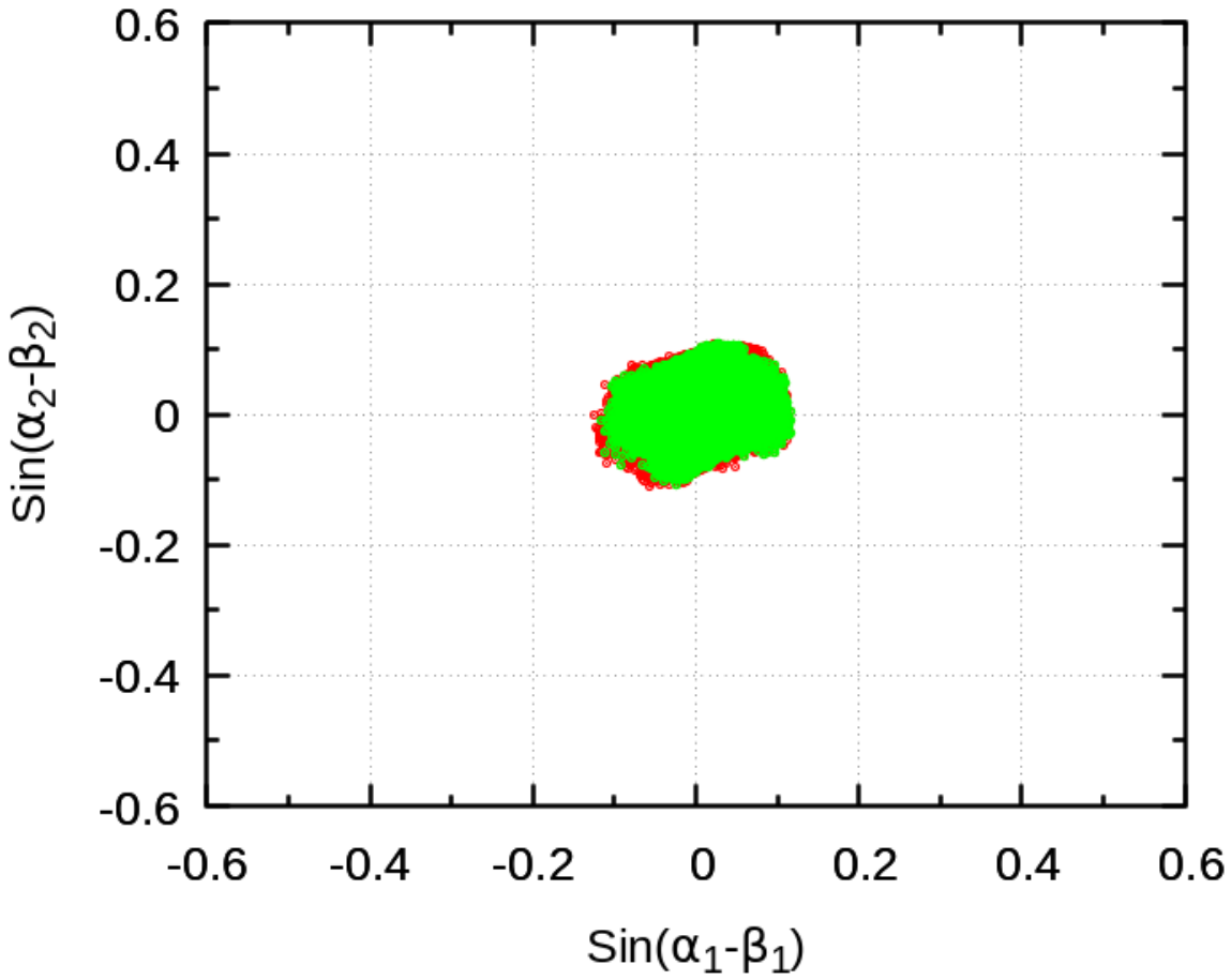
To study the allowed regions for the cross section ratios $\mu_{if}^{h}$ , we follow Fontes:2014xva; Barroso:2012wz and calculate each $\mu_{if}^{h}$ using all production channels. Our set of points is then shown in Figs. 3 - 6. Similar to the complex 2HDM analyzed by Fontes, Romão and Silva in Fontes:2014xva, there is a strong correlation between $\mu_{Z\gamma}$ and $\mu_{\gamma\gamma}$ in our Type-Z model, as shown in Fig. 6.

Such a correlation is also visible between $\mu_{ZZ}$ and $\mu_{\gamma\gamma}$ in Fig. 3. It is less apparent in correlations with $\tau^{+}\tau^{-}$ and $b\bar{b}$ , as shown in Figs. 4 and 5.

IV Calculation of the BR( $B\to X_{s}\gamma$ )

IV.1 Introduction

It is well known that the experimental bounds on $B\to X_{s}\gamma$ place stringent restrictions on the parameter space of models with charged scalars Borzumati:1998tg; Borzumati:1998nx; Misiak:2017bgg; Misiak:2018cec; Akeroyd:2020nfj. Most notably, there is a bound on the mass of the only charged Higgs boson present in the Type-II 2HDM which, at 95% CL (2 $\sigma$ ), is according to Misiak:2017bgg

m_{H^{+}}>580\,\text{GeV}\,.

(63)

The exact value for this bound depends on both the theoretical approximations Bernlochner:2020jlt and the experimental errors. The experimental average gives Amhis:2019ckw

\text{BR}^{\rm exp}(B\to X_{s}\gamma)=(3.32\pm 0.15)\times 10^{-4}\,,

(64)

while the NNLO calculation within the SM yields Misiak:2020vlo; Akeroyd:2020nfj

\text{BR}^{\rm SM}(B\to X_{s}\gamma)=(3.40\pm 0.17)\times 10^{-4}\,,

(65)

with an error of about 5%.

As explained below, we will take an error of 2.5% around the central value of the calculation and, following Akeroyd:2020nfj, we consider 99% CL (3 $\sigma$ ) for the experimental error:

2.87\times 10^{-4}<\text{BR}(B\to X_{s}\gamma)<3.77\times 10^{-4}\,.

(66)

IV.2 The calculation

We follow closely the calculation by Borzumati and Greub in Ref. Borzumati:1998tg. There, the new contributions from the charged Higgs bosons are encoded in the Wilson coefficients,


$\displaystyle C^{0,{\rm eff}}_{7}(\mu_{W})=$	$\displaystyle C^{0,{\rm eff}}_{7,\rm SM}(\mu_{W})+\|Y\|^{2}C^{0,{\rm eff}}_{7,\rm YY}(\mu_{W})+(XY^{*})C^{0,{\rm eff}}_{7,\rm XY}(\mu_{W})\,,$	(67a)
$\displaystyle C^{0,{\rm eff}}_{8}(\mu_{W})=$	$\displaystyle C^{0,{\rm eff}}_{8,\rm SM}(\mu_{W})+\|Y\|^{2}C^{0,{\rm eff}}_{8,\rm YY}(\mu_{W})+(XY^{*})C^{0,{\rm eff}}_{8,\rm XY}(\mu_{W})\,,$	(67b)
$\displaystyle C^{1,{\rm eff}}_{4}(\mu_{W})=$	$\displaystyle E_{0}(x)+\frac{2}{3}\log\left(\frac{\mu_{W}^{2}}{M_{W}^{2}}\right)+\|Y\|^{2}E_{H}(y)\,,$	(67c)
$\displaystyle C^{1,{\rm eff}}_{7}(\mu_{W})=$	$\displaystyle C^{1,{\rm eff}}_{7,\rm SM}(\mu_{W})+\|Y\|^{2}C^{1,{\rm eff}}_{7,\rm YY}(\mu_{W})+(XY^{*})C^{1,{\rm eff}}_{7,\rm XY}(\mu_{W})\,,$	(67d)
$\displaystyle C^{1,{\rm eff}}_{8}(\mu_{W})=$	$\displaystyle C^{1,{\rm eff}}_{8,\rm SM}(\mu_{W})+\|Y\|^{2}C^{1,{\rm eff}}_{8,\rm YY}(\mu_{W})+(XY^{*})C^{1,{\rm eff}}_{8,\rm XY}(\mu_{W})\,,$	(67e)

where we are using the notation in Ref. Borzumati:1998tg which should be consulted for the definitions and also for the procedure used in evolving the coefficients to the scale $\mu_{b}=m_{b}$ . The dependence on the charged Higgs mass appears because the functions $C^{0,{\rm eff}}_{i,\rm YY},C^{0,{\rm eff}}_{i,\rm XY},C^{1,{\rm eff}}_{i,\rm YY}$ , and $C^{1,{\rm eff}}_{i,\rm XY}$ depend on $y=m_{t}^{2}/m_{H^{+}}^{2}$ , while the SM coefficients depend on $x=m_{t}^{2}/M_{W}^{2}$ .

For models with multiple charged Higgs there is one contribution (and one parameter $y_{k}$ ) for each particle. A model with two charged Higgs is discussed in Akeroyd:2020nfj; Logan:2020mdz, with interesting earlier work highlighting the possible cancellation between the two charged Higgs contributions appearing in Refs. Hewett:1994bd; Akeroyd:2016ssd. We obtain, for example,

	$\displaystyle C^{1,{\rm eff}}_{7}(\mu_{W})=$	$\displaystyle C^{1,{\rm eff}}_{7,\rm SM}(\mu_{W})+\|Y_{1}\|^{2}C^{1,{\rm eff}}_{7,\rm YY}(\mu_{W},y_{1})+\|Y_{2}\|^{2}C^{1,{\rm eff}}_{7,\rm YY}(\mu_{W},y_{2})$
		$\displaystyle+(X_{1}Y_{1}^{})C^{1,{\rm eff}}_{7,\rm XY}(\mu_{W},y_{1})+(X_{2}Y_{2}^{})C^{1,{\rm eff}}_{7,\rm XY}(\mu_{W},y_{2})\,,$		(68)

where we wrote explicitly the dependence on the charged Higgs masses,

y_{1}=\frac{m_{t}^{2}}{m_{H_{1}^{+}}^{2}},\quad y_{2}=\frac{m_{t}^{2}}{m_{H_{2}^{+}}^{2}}\,,

(69)

and used

X_{1}=-\frac{\textbf{Q}_{22}}{\cos\beta_{2}\sin\beta_{1}},\quad Y_{1}=\frac{\textbf{Q}_{23}}{\sin\beta_{2}},\quad X_{2}=-\frac{\textbf{Q}_{32}}{\cos\beta_{2}\,\sin\beta_{1}},\quad Y_{2}=\frac{\textbf{Q}_{33}}{\sin\beta_{2}}.

(70)

We took the input parameters from Ref. Borzumati:1998tg except for $\alpha_{s}(M_{Z}),m_{t},M_{Z},M_{W}$ , that were updated to the most recent values of the Particle Data Group Zyla:2020zbs:⁵⁵ 5 If we use exclusively the input values of Ref. Borzumati:1998tg, we reproduce their SM results. We are extremely grateful to C. Greub for discussions and for providing us with the original code used in Borzumati:1998tg, utilized to cross check our independent calculations.


$\displaystyle\alpha_{s}(M_{Z})=0.1179\pm 0.0010,$	$\displaystyle m_{t}=172.76\pm 0.3\,\text{GeV},$	(71a)
$\displaystyle m_{c}/m_{b}=0.29\pm 0.02,$	$\displaystyle m_{b}-m_{c}=3.39\pm 0.04\,\text{GeV},$	(71b)
$\displaystyle\alpha_{em}^{-1}=137.036,$	$\displaystyle\|V_{ts}^{*}V_{tb}/V_{cb}\|^{2}=0.95\pm 0.03,$	(71c)
$\displaystyle\text{BR}_{SL}=0.1049\pm 0.0046\,.$		(71d)

V Impact of $b\rightarrow s\gamma$ on the $\mathbbm{Z}_{3}$ 3HDM parameter space

We find that much of the parameter space considered in Ref. Chakraborti:2021bpy is forbidden. This is most apparent by considering their Fig. 2, which we turn to next.

V.1 Only $b\to s\gamma$

On Fig. 2 of Ref. Chakraborti:2021bpy the parameters are fixed as

\tan\beta_{1}=10,\quad\tan\beta_{2}=2,\quad\gamma_{2}=\frac{\pi}{6},\frac{\pi}{4},\frac{\pi}{3}\,,

(72)

while imposing

m_{h_{2}}=m_{A_{1}}=m_{H_{1}^{+}},\quad m_{h_{3}}=m_{A_{2}}=m_{H_{2}^{+}},\quad\alpha_{1}=\beta_{1},\alpha_{2}=\beta_{2},\gamma_{1}=\gamma_{2}=-\alpha_{3}\,.

(73)

Applying only the $b\to s\gamma$ cut we reproduce their Fig. 2 in our Fig. 7.

Fig. 7 passes all theoretical constraints, even including unitarity and BFB.

V.2 The effect of other constraints

From the previous plots, the conclusion that we can have one of the charged Higgs relatively light if the other is sufficiently heavy seems correct. However we now show that for this choice of parameters this is not the case. With the choice of Eqs. (72)-(73, the bounds from the decays of the 125 GeV Higgs are simply satisfied. However the same is not true for current bounds on heavier scalars. Indeed, every single point in Fig. 7 is excluded by HB5; not a single point remains. This will be explained in detail in the following section.

V.3 Enlarging the region of good points

We discovered that the situation described in the previous section is a consequence of the small range chosen for $\gamma_{2}$ . To illustrate this, we kept the other conditions in Eqs. (72)-(73), but allowed for

\gamma_{2}\in[-\pi/2,\pi/2]\,,

(74)

and (for Fig. 8) also varied $\tan{\beta_{1}}$ . The points which survive HiggsBounds-5.9.1 are shown in dark green on the left panel of Fig. 8.

The allowed points for $\tan{\beta_{1}}=10$ are concentrated around $\gamma_{2}=0,\pm\pi/2$ , excluding $\gamma_{2}=\pi/6,\pi/4,\pi/3$ . Taking the interval in Eq. (74) one can indeed find regions of good points.⁶⁶ 6 This it true regardless of whether or not we vary $\beta_{1}$ , as long as we enlarge the region of $\gamma_{2}$ .

It is interesting to compare with what happens with the previous version of HiggsBounds-5.7.1, shown on the right panel of Fig. 8. For that case there are many points allowed for all values of $\gamma_{2}$ , even for $\tan{\beta_{1}}=10$ . We have found that this is due to the recent bounds on $h_{2,3}\rightarrow\tau^{+}\tau^{-}$ decay in Ref. ATLAS:2020zms, included in HiggsBounds-5.9.1 but not in HiggsBounds-5.7.1, which used the previous bounds CMS:2015mca; CMS:2017epy.⁷⁷ 7 In Ref. Chakraborti:2021bpy the strong constraints from neutral scalar decays into $\tau\tau$ still seemed to allow points with the choices in Eqs. (72)-(73).

To better illuminate this point, we show $\sigma(pp\to h_{2})\times\text{BR}(h_{2}\to\tau\tau)$ versus $m_{h_{2}}$ in Fig. 9. In this figure, the parameters are as in Eqs. (72)-(73, except that $\gamma_{2}\in[-\pi/2,\pi/2]$ . Points in cyan are points that pass all constraints before HiggsBounds. In light green are the points in the restricted interval $\gamma_{2}\in[\pi/6,\pi/3]$ . In the left panel points in dark green are those who survided after HiggsBounds-5.7.1. In the right panel we have the same situation but now we used HiggsBounds-5.9.1. We see that there were good points in the restricted interval $\gamma_{2}\in[\pi/6,\pi/3]$ in the left panel, but they disappeared with the newer version HiggsBounds-5.9.1. We have confirmed that similar plots can be obtained for $h_{3}$ .

This is a good point to stress again the role that the LHC is having in constraining models with new scalar physics. One sees the strong impact that the updated LHC results have in constraining the $\mathbbm{Z}_{3}$ 3HDM. This highlights the importance that the new LHC run will have in constraining the parameter space of extended scalar sectors.

To better understand the behaviour of $\sigma(pp\to h_{i})\times\text{BR}(h_{i}\to\tau\tau)$ ( $i=2,3$ ) we can make the simplified assumption⁸⁸ 8 We are neglecting the dependence of the cross section on the mass. that this product is proportional to

\sigma(pp\to h_{i})\times\text{BR}(h_{i}\to\tau\tau)\propto g_{h_{i}\tau\tau}^{2}\,g_{h_{i}tt}^{2}\equiv f_{i}\ ,

(75)

where we are assuming that the production occurs mainly via gluon fusion with the top quark in the loop. Now, using the assumptions of Eq. (73) in Eq. (25), we have

		$\displaystyle g_{h_{2}\tau\tau}=-\frac{c_{\alpha_{3}}t_{\beta_{1}}}{c_{\alpha_{2}}}-s_{\alpha_{3}}t_{\beta_{2}}=-\frac{t_{\beta_{1}}}{c_{\beta_{2}}}\,c_{\gamma_{2}}+t_{\beta_{2}}s_{\gamma_{2}}\,,$		$\displaystyle g_{h_{2}tt}=\frac{c_{\alpha_{2}}s_{\alpha_{3}}}{s_{\beta_{2}}}=-\frac{1}{t_{\beta_{2}}}\,s_{\gamma_{2}}\ ,$
		$\displaystyle g_{h_{3}\tau\tau}=-c_{\alpha_{3}}t_{\beta_{2}}+\frac{s_{\alpha_{3}}t_{\beta_{1}}}{c_{\alpha_{2}}}=-t_{\beta_{2}}c_{\gamma_{2}}-\frac{t_{\beta_{1}}}{c_{\beta_{2}}}s_{\gamma_{2}}\,,$		$\displaystyle g_{h_{3}tt}=\frac{c_{\alpha_{2}}c_{\alpha_{3}}}{s_{\beta_{2}}}=\frac{1}{t_{\beta_{2}}}\,c_{\gamma_{2}}\ ,$		(76)

where, for Fig. 9, $\beta_{1},\beta_{2}$ are fixed and $\gamma_{2}\in[-\pi/2,\pi/2]$ . Fig. 10 shows the functions in Eq. (75) – $f_{2}$ for $h_{2}$ and $f_{3}$ for $h_{3}$ – for $\tan{\beta_{1}}=10$ and $\tan{\beta_{2}}=2$ as in Eq. (72), but keeping $\gamma_{2}$ free.

Figure 10: Graphic of the functions

f_{j}

defined in Eq. (75) for varying

\gamma_{2}=-\alpha_{3}

, with

\tan{\beta_{1}}=10

and

\tan{\beta_{2}}=2

. Function

f_{2}

(

f_{3}

) in black/solid (blue/dashed) line.

We see that these functions are largest precisely in the approximate interval $\pm\gamma_{2}\in[\pi/6,\pi/3]$ . This explains why these points are the first to be excluded by the bounds on $\sigma(pp\to h_{2})\times\text{BR}(h_{2}\to\tau\tau)$ , and why, going outside such bounds, some points can be preserved.⁹⁹ 9 Of course, we have ignored in this simple reasoning the dependence on $m_{h_{i}}$ , which has been taken into account appropriately in our scans and HB5 limits.

V.4 The effect of $\tan\beta$ ’s

In the last section we saw that while maintaining the main features of Eqs. (72)-(73, but enlarging the range of variation of $\gamma_{2}$ , we could find points allowed by all current experimental constraints. Here we exploit the variation of both $\tan\beta$ ’s in the range

\tan\beta_{1,2}\in[10^{-0.5},10]\,,

(77)

subject to the condition of perturbativity of the Yukawa couplings in Eq. (52). The result is shown in Fig. 11.

We see that by varying the range of $\tan\beta$ ’s we can have smaller masses for the charged Higgs bosons. For $\tan\beta<1$ it is even possible to have both charged Higgs with masses below 400 GeV.

VI Going beyond exact alignment

We have performed a completely uniform scan and found out that very few points survived and those were not too far away from the alignment condition of Eq. (73). So another strategy can be to scan points that differ from the perfect alignment of Eq. (73) by 1% or 10%.

In Fig. 12 we show the results for the case when we allow the parameters to differ 1% from the perfect alignment limit.

Next we considered the case when the difference for perfect alignment was 10%. This is shown in Fig. 13.

We see that the acceptable points which differ more from perfect alignment are less frequent, as expected.¹⁰¹⁰ 10 To be more specific, for the same number of points generated with the constraint of alignment within 10% or 1%, fewer of the former are obtained which pass all requirements. Nevertheless, one can still find many points which differ from exact alignment by as much as 10%, while satisfying all experimental and theoretical constraints. And such points do allow for qualitatively different predictions, as we saw when looking at the charged scalar masses consistent with $b\rightarrow s\gamma$ . We conclude that imposing perfect alignment is too constraining and does not cover all the interesting features of the $\mathbbm{Z}_{3}$ 3HDM.

VI.1 Unusual signals of charged scalars

As we have seen, the contributions of the two charged scalars can exhibit large cancellations in the decays $h\rightarrow\gamma\gamma$ and $B\rightarrow X_{s}\gamma$ .¹¹¹¹ 11 For 3HDMs, the cancellation can be exact in $B\rightarrow X_{s}\gamma$ because there are two charged components of Higgs doublets feeding the two physical charged Higgs states. This is no longer the case in the Zee model, with two Higgs doublets and one charged scalar singlet Florentino:2021ybj. For some choices of parameter space, it is even possible that there are cancellations in both decays simultaneously. This is illustrated in Fig. 14.

Such charged scalars would, thus, be difficult to probe indirectly.

Notice that points with exact alignment, in cyan in Fig. 14, do not allow for cancellation in $h\to\gamma\gamma$ ; but alignment with 1% already does.

Most points within the blue box close to (0,0) have $H_{2}^{+}$ decays into quarks or leptons, which are being sought at LHC. But there are points which could also be difficult to probe directly with such common searches, even tough one or both charged scalars might have relatively small masses. Indeed, one can find fine-tuned points in parameter space where the $H_{2}^{+}$ does not decay primordially into quarks or leptons, but rather as $H_{2}^{+}\rightarrow H_{1}^{+}h_{j}$ with $h_{j}=h_{1},h_{2},A_{1}$ . We propose that such decays be actively searched for at LHC’s next run. To aid in that experimental endeavour, we present some benchmark points (BP) in the next section.

VII Illustrative benchmark points

This section is devoted to some benchmark points/lines, with features which may prove useful for the experimental searches.

There has been a recent interest in the literature for unusual decays of the charged Higgs Bahl:2021str, specially those in which the charged Higgs decays to $W^{+}h_{i}$ where $h_{i}$ is any of the scalars or pseudo scalars in the model.

We have performed a search in our large data sets and found many points where BR( $H_{1}^{+}\to W^{+}+h_{125}$ ) was larger than 80%. From those we selected three benchmark points (BP) that we list in table 1.

Type-Z	BP1	BP2	BP3
$m_{h_{2}}$	419.00	494.60	486.26
$m_{h_{3}}$	799.60	850.88	694.44
$m_{A_{1}}$	413.80	483.96	513.46
$m_{A_{2}}$	763.15	806.44	647.56
$m_{H_{1}^{\pm}}$	396.13	477.63	506.36
$m_{H_{2}^{\pm}}$	752.81	843.034	654.77
$(m_{12}^{2})$	-8350	-31768	-19562
$(m_{13}^{2})$	-83278	-80800	-63134
$(m_{23}^{2})$	-231428	-232361	-197019
$\alpha_{1}$	1.289	1.343	1.328
$\alpha_{2}$	0.5419	0.4406	0.7119
$\alpha_{3}$	0.00543	-0.00299	0.01136
$\gamma_{1}$	-0.00503	0.00322	-0.01078
$\gamma_{2}$	-0.00504	0.00301	-0.01011
$\beta_{1}$	1.192	1.263	1.231
$\beta_{2}$	0.5077	0.4311	0.7351
BR( $H_{1}^{+}\rightarrow\nu_{\tau}+\tau^{+}$ )	0.0688	0.0790	0.0784
BR( $H_{1}^{+}\rightarrow t+\bar{b}$ )	0.0383	0.0197	0.0358
BR( $H_{1}^{+}\rightarrow W^{+}h_{1}$ )	0.8926	0.9011	0.8855
BR( $H_{2}^{+}\rightarrow t+\bar{b}$ )	0.9970	0.9995	0.9965
BR( $H_{2}^{+}\rightarrow W^{+}h_{1}$ )	0.0012	0.0001	0.0009
BR( $H_{2}^{+}\rightarrow W^{+}h_{2}$ )	0.0007	0.0003	0.0006

Table 1: Benchmark points for the Type Z

Z_{3}

-3HDM.

For each of these BP we let the mass of the $H_{1}^{+}$ vary, leaving all the other parameters fixed, obtaining benchmark lines. All these points verify all the constraints, including those from HiggsBounds-5.9.1. These BP all have the characteristic that the dominant decay of the charged $H_{1}^{+}$ is not in the $tb$ channel, but in $W^{+}h_{125}$ , which makes these interesting and deserving to be searched at the LHC.

Notice that, for these BP, the other charged Higgs decays 100% in $tb$ . For BP2 the decay $H_{1}^{+}\to W^{+}A_{1}$ opens up when the mass of the $H_{1}^{+}$ is such that $m_{H_{1}^{+}}>M_{W}+m_{A_{1}}$ explaining the decrease in our prefered branching ratio (see Fig. ). The same happens for the channel $H_{1}^{+}\to W^{+}h_{2}$ for BP3 as can be seen in Fig. 16.

VIII Conclusions

Multi Higgs models with $N\geq 3$ allow for the possibility that all fermions of a given charge couple exclusively to one dedicated scalar. These are known as Type-Z models, and constitute a fifth alternative beyond the four natural flavour conservation models allowed in the 2HDM. We investigate the current bounds on the Type-Z 3HDM imposed by a $\mathbbm{Z}_{3}$ symmetry. We perform an up-to-date analysis including the latest data for the 125GeV Higgs Aad:2019mbh, bounds on new scalars through the HiggsBounds-5.9.1 code Bechtle:2020pkv, and the very important theoretical constraints.

We use the theoretical bounds from unitarity Bento:2017eti and BFB; the latter developed here for the first time. We stress the importance of using the most recent LHC bounds, which constrain severely the allowed parameter space. In particular, we show that bounds from $h_{2}\rightarrow\tau^{+}\tau^{-}$ alter significantly some results in the literature Chakraborti:2021bpy. This is clearly visible in our Fig. 8 and Fig. 9. Moreover, we also stress the fact that interesting physical observables may differ significantly when one considers situations close to the alignment limit, versus adopting the exact alignment limit. Indeed, current LHC bounds on the productions and branching ratios of the 125GeV neutral scalar force the measured couplings to lie close to those obtained for the SM Higgs. Nevertheless, forcing those couplings to match exactly those in the SM is too constraining on the parameter space and precludes much of the interesting new features that the $\mathbbm{Z}_{3}$ 3HDM has.

We look at the constraints allowed by current data on the 125GeV Higgs decays, including a detailed look at $h\to\gamma\gamma$ and its correlations with the other decays. We point out the possibility that the contributions from the two charged scalars might cancel in $h\to\gamma\gamma$ . This is also possible in $B\to X_{s}\gamma$ , and we explore explicitly how this allows for lower masses for the charged scalars. We provide illustrative benchmark points to aid in experimental searches. By comparing the constraints from HiggsBounds-5.7.1 and the newer HiggsBounds-5.9.1 we highlight the importance that the next LHC run will have in further constraining this model, or perhaps, finally uncovering new physics in the scalar sector.

Acknowledgments

We are very grateful to D. Das for detailed discussions regarding his Ref.Chakraborti:2021bpy. We are also very grateful to C. Greub for detailed discussions regarding his Refs. Borzumati:1998tg; Borzumati:1998nx. JPS is grateful to Z. Ligeti for discussions. This work is supported in part by the Portuguese Fundação para a Ciência e Tecnologia (FCT) under Contracts CERN/FIS-PAR/0008/2019, PTDC/FIS-PAR/29436/2017, UIDB/00777/2020, and UIDP/00777/2020; these projects are partially funded through POCTI (FEDER), COMPETE, QREN, and the EU.

Appendix A Some important couplings

This appendix is devoted to some important couplings for the $\mathbbm{Z}_{3}$ 3HDM used in our calculations. In our conventions these couplings include the $i$ from the Feynman rules. These couplings were derived with the help of the software FeynMasterFontes:2019wqh; Fontes:2021iue.

A.1 Scalar couplings to $W^{\pm}$ bosons

We find for the neutral scalar couplings to $W^{+}W^{-}$ ,

\displaystyle[h_{j},W^{+}_{\nu},W^{-}_{\rho}]=ig\,M_{W}\,g_{\nu\rho}\,\left(\vbox to12.0pt{}{R_{j1}}\,{\hat{v}_{1}}+{R_{j2}}\,{\hat{v}_{2}}+{R_{j3}}\,{\hat{v}_{3}}\right)

(78)

Thus,

C_{j}=R_{j1}\hat{v}_{1}+R_{j2}\hat{v}_{2}+R_{j3}\hat{v}_{3}\,,

(79)

is to be used in Eq. (56).

A.2 Scalar couplings to charged Higgs

The couplings of the scalars $h_{j}$ with $j=1,2,3$ to the charged Higgs $H_{k-1}^{\mp},H_{l-1}^{\pm}$ where $k,l=2,3$ (we do not consider here the charged Goldstone) are,

$\displaystyle[h_{j},H_{k^{\prime}}^{\mp},H_{l^{\prime}}^{\pm}]=\frac{-i}{2}\,v$	$\displaystyle\left[\vbox to14.0pt{}4\,{\lambda_{1}}\,{Q_{k1}}\,{Q_{l1}}\,{R_{j1}}\,{\hat{v}_{1}}+2\,{\lambda_{5}}\,{Q_{k3}}\,{Q_{l3}}\,{R_{j1}}\,{\hat{v}_{1}}+{\lambda_{7}}\,{Q_{k2}}\,{Q_{l1}}\,{R_{j2}}\,{\hat{v}_{1}}\right.$
	$\displaystyle\left.+{\lambda_{10}}\,{Q_{k3}}\,{Q_{l1}}\,{R_{j2}}\,{\hat{v}_{1}}+{\lambda_{7}}\,{Q_{k1}}\,{Q_{l2}}\,{R_{j2}}\,{\hat{v}_{1}}+{\lambda_{11}}\,{Q_{k3}}\,{Q_{l2}}\,{R_{j2}}\,{\hat{v}_{1}}\right.$
	$\displaystyle\left.+{\lambda_{10}}\,{Q_{k1}}\,{Q_{l3}}\,{R_{j2}}\,{\hat{v}_{1}}+{\lambda_{11}}\,{Q_{k2}}\,{Q_{l3}}\,{R_{j2}}\,{\hat{v}_{1}}+{\lambda_{10}}\,{Q_{k2}}\,{Q_{l1}}\,{R_{j3}}\,{\hat{v}_{1}}\right.$
	$\displaystyle\left.+{\lambda_{8}}\,{Q_{k3}}\,{Q_{l1}}\,{R_{j3}}\,{\hat{v}_{1}}+{\lambda_{10}}\,{Q_{k1}}\,{Q_{l2}}\,{R_{j3}}\,{\hat{v}_{1}}+{\lambda_{12}}\,{Q_{k3}}\,{Q_{l2}}\,{R_{j3}}\,{\hat{v}_{1}}\right.$
	$\displaystyle\left.+{\lambda_{8}}\,{Q_{k1}}\,{Q_{l3}}\,{R_{j3}}\,{\hat{v}_{1}}+{\lambda_{12}}\,{Q_{k2}}\,{Q_{l3}}\,{R_{j3}}\,{\hat{v}_{1}}+{\lambda_{7}}\,{Q_{k2}}\,{Q_{l1}}\,{R_{j1}}\,{\hat{v}_{2}}\right.$
	$\displaystyle\left.+{\lambda_{10}}\,{Q_{k3}}\,{Q_{l1}}\,{R_{j1}}\,{\hat{v}_{2}}+{\lambda_{7}}\,{Q_{k1}}\,{Q_{l2}}\,{R_{j1}}\,{\hat{v}_{2}}+{\lambda_{11}}\,{Q_{k3}}\,{Q_{l2}}\,{R_{j1}}\,{\hat{v}_{2}}\right.$
	$\displaystyle\left.+{\lambda_{10}}\,{Q_{k1}}\,{Q_{l3}}\,{R_{j1}}\,{\hat{v}_{2}}+{\lambda_{11}}\,{Q_{k2}}\,{Q_{l3}}\,{R_{j1}}\,{\hat{v}_{2}}+4\,{\lambda_{2}}\,{Q_{k2}}\,{Q_{l2}}\,{R_{j2}}\,{\hat{v}_{2}}\right.$
	$\displaystyle\left.+2\,{\lambda_{6}}\,{Q_{k3}}\,{Q_{l3}}\,{R_{j2}}\,{\hat{v}_{2}}+{\lambda_{11}}\,{Q_{k2}}\,{Q_{l1}}\,{R_{j3}}\,{\hat{v}_{2}}+{\lambda_{12}}\,{Q_{k3}}\,{Q_{l1}}\,{R_{j3}}\,{\hat{v}_{2}}\right.$
	$\displaystyle\left.+{\lambda_{11}}\,{Q_{k1}}\,{Q_{l2}}\,{R_{j3}}\,{\hat{v}_{2}}+{\lambda_{9}}\,{Q_{k3}}\,{Q_{l2}}\,{R_{j3}}\,{\hat{v}_{2}}+{\lambda_{12}}\,{Q_{k1}}\,{Q_{l3}}\,{R_{j3}}\,{\hat{v}_{2}}\right.$
	$\displaystyle\left.+{\lambda_{9}}\,{Q_{22}}\,{Q_{l3}}\,{R_{j3}}\,{\hat{v}_{2}}+2\,{\lambda_{4}}\,\left({Q_{22}}\,{Q_{l2}}\,{R_{j1}}\,{\hat{v}_{1}}+{Q_{k1}}\,{Q_{l1}}\,{R_{j2}}\,{\hat{v}_{2}}\right)\right.$
	$\displaystyle\left.+{\lambda_{10}}\,{Q_{22}}\,{Q_{l1}}\,{R_{j1}}\,{\hat{v}_{3}}+{\lambda_{8}}\,{Q_{k3}}\,{Q_{l1}}\,{R_{j1}}\,{\hat{v}_{3}}+{\lambda_{10}}\,{Q_{k1}}\,{Q_{l2}}\,{R_{j1}}\,{\hat{v}_{3}}\right.$
	$\displaystyle\left.+{\lambda_{12}}\,{Q_{k3}}\,{Q_{l2}}\,{R_{j1}}\,{\hat{v}_{3}}+{\lambda_{8}}\,{Q_{k1}}\,{Q_{l3}}\,{R_{j1}}\,{\hat{v}_{3}}+{\lambda_{12}}\,{Q_{22}}\,{Q_{l3}}\,{R_{j1}}\,{\hat{v}_{3}}\right.$
	$\displaystyle\left.+{\lambda_{11}}\,{Q_{22}}\,{Q_{l1}}\,{R_{j2}}\,{\hat{v}_{3}}+{\lambda_{12}}\,{Q_{k3}}\,{Q_{l1}}\,{R_{j2}}\,{\hat{v}_{3}}+{\lambda_{11}}\,{Q_{k1}}\,{Q_{l2}}\,{R_{j2}}\,{\hat{v}_{3}}\right.$
	$\displaystyle\left.+{\lambda_{9}}\,{Q_{k3}}\,{Q_{l2}}\,{R_{j2}}\,{\hat{v}_{3}}+{\lambda_{12}}\,{Q_{k1}}\,{Q_{l3}}\,{R_{j2}}\,{\hat{v}_{3}}+{\lambda_{9}}\,{Q_{22}}\,{Q_{l3}}\,{R_{j2}}\,{\hat{v}_{3}}\right.$
	$\displaystyle\left.+2\,{\lambda_{5}}\,{Q_{k1}}\,{Q_{l1}}\,{R_{j3}}\,{\hat{v}_{3}}+2\,{\lambda_{6}}\,{Q_{22}}\,{Q_{l2}}\,{R_{j3}}\,{\hat{v}_{3}}\right.$
	$\displaystyle\left.+4\,{\lambda_{3}}\,{Q_{k3}}\,{Q_{l3}}\,{R_{j3}}\,{\hat{v}_{3}}\vbox to14.0pt{}\right]$
$\displaystyle\hskip-14.22636pt\equiv$	$\displaystyle\,i\,v\,\lambda_{h_{j},H_{k^{\prime}}^{+},H_{l^{\prime}}^{-}}\,,$	(80)

where we have defined $k^{\prime}\equiv k-1$ , $l^{\prime}\equiv l-1$ with $j=1,2,3$ and $k,l=2,3$ . Recall that $\hat{v}_{k}=v_{k}/v$ . The coupling $\lambda_{h_{j},H_{k^{\prime}}^{+},H_{l^{\prime}}^{-}}$ is to be used in Eq. (57).

A.3 Pseudoscalar couplings to charged Higgs

The couplings of the pseudoscalars $A_{j^{\prime}}$ with $j^{\prime}=j-1$ and $j=2,3$ (we do not consider the coupling of the neutral Goldstone) are

$\displaystyle[A_{j^{\prime}},H_{1}^{\mp},H_{2}^{\pm}]=$	$\displaystyle\pm\frac{1}{2}\,v\left[\vbox to14.0pt{}{\lambda_{8}}\,{P_{j3}}\,{Q_{23}}\,{Q_{31}}\,{\hat{v}_{1}}+{\lambda_{11}}\,{P_{j2}}\,{Q_{23}}\,{Q_{32}}\,{\hat{v}_{1}}-{\lambda_{12}}\,{P_{j3}}\,{Q_{23}}\,{Q_{32}}\,{\hat{v}_{1}}\right.$
	$\displaystyle\left.-{\lambda_{8}}\,{P_{j3}}\,{Q_{21}}\,{Q_{33}}\,{\hat{v}_{1}}-{\lambda_{11}}\,{P_{j2}}\,{Q_{22}}\,{Q_{33}}\,{\hat{v}_{1}}+{\lambda_{12}}\,{P_{j3}}\,{Q_{22}}\,{Q_{33}}\,{\hat{v}_{1}}\right.$
	$\displaystyle\left.+{\lambda_{11}}\,{P_{j3}}\,{Q_{22}}\,{Q_{31}}\,{\hat{v}_{2}}-{\lambda_{12}}\,{P_{j3}}\,{Q_{23}}\,{Q_{31}}\,{\hat{v}_{2}}-{\lambda_{11}}\,{P_{j3}}\,{Q_{21}}\,{Q_{32}}\,{\hat{v}_{2}}\right.$
	$\displaystyle\left.-{\lambda_{11}}\,{P_{j1}}\,{Q_{23}}\,{Q_{32}}\,{\hat{v}_{2}}+{\lambda_{9}}\,{P_{j3}}\,{Q_{23}}\,{Q_{32}}\,{\hat{v}_{2}}+{\lambda_{12}}\,{P_{j3}}\,{Q_{21}}\,{Q_{33}}\,{\hat{v}_{2}}\right.$
	$\displaystyle\left.+{\lambda_{11}}\,{P_{j1}}\,{Q_{22}}\,{Q_{33}}\,{\hat{v}_{2}}-{\lambda_{9}}\,{P_{j3}}\,{Q_{22}}\,{Q_{33}}\,{\hat{v}_{2}}\right.$
	$\displaystyle\left.+{\lambda_{7}}\,\left({Q_{22}}\,{Q_{31}}-{Q_{21}}\,{Q_{32}}\right)\,\left({P_{j2}}\,{\hat{v}_{1}}-{P_{j1}}\,{\hat{v}_{2}}\right)-{\lambda_{11}}\,{P_{j2}}\,{Q_{22}}\,{Q_{31}}\,{\hat{v}_{3}}\right.$
	$\displaystyle\left.-{\lambda_{8}}\,{P_{j1}}\,{Q_{23}}\,{Q_{31}}\,{\hat{v}_{3}}+{\lambda_{12}}\,{P_{j2}}\,{Q_{23}}\,{Q_{31}}\,{\hat{v}_{3}}+{\lambda_{11}}\,{P_{j2}}\,{Q_{21}}\,{Q_{32}}\,{\hat{v}_{3}}\right.$
	$\displaystyle\left.+{\lambda_{12}}\,{P_{j1}}\,{Q_{23}}\,{Q_{32}}\,{\hat{v}_{3}}-{\lambda_{9}}\,{P_{j2}}\,{Q_{23}}\,{Q_{32}}\,{\hat{v}_{3}}+{\lambda_{8}}\,{P_{j1}}\,{Q_{21}}\,{Q_{33}}\,{\hat{v}_{3}}\right.$
	$\displaystyle\left.-{\lambda_{12}}\,{P_{j2}}\,{Q_{21}}\,{Q_{33}}\,{\hat{v}_{3}}-{\lambda_{12}}\,{P_{j1}}\,{Q_{22}}\,{Q_{33}}\,{\hat{v}_{3}}+{\lambda_{9}}\,{P_{j2}}\,{Q_{22}}\,{Q_{33}}\,{\hat{v}_{3}}\right.$
	$\displaystyle\left.+{\lambda_{10}}\,\left(\vbox to11.0pt{}-{P_{j3}}\,{Q_{22}}\,{Q_{31}}\,{\hat{v}_{1}}-{P_{j2}}\,{Q_{23}}\,{Q_{31}}\,{\hat{v}_{1}}+{P_{j3}}\,{Q_{21}}\,{Q_{32}}\,{\hat{v}_{1}}\right.\right.$
	$\displaystyle\left.\left.+{P_{j2}}\,{Q_{21}}\,{Q_{33}}\,{\hat{v}_{1}}+{P_{j1}}\,{Q_{23}}\,{Q_{31}}\,{\hat{v}_{2}}-{P_{j1}}\,{Q_{21}}\,{Q_{33}}\,{\hat{v}_{2}}\right.\right.$
	$\displaystyle\left.\left.+{P_{j1}}\,{Q_{22}}\,{Q_{31}}\,{\hat{v}_{3}}-{P_{j1}}\,{Q_{21}}\,{Q_{32}}\,{\hat{v}_{3}}\vbox to11.0pt{}\right)\vbox to14.0pt{}\right],$
$\displaystyle\equiv$	$\displaystyle\,v\,\lambda_{A_{j^{\prime}}H_{1}^{\mp}H_{2}^{\pm}}\,,$	(81)

for $j^{\prime}=j-1$ and $j=2,3$ . Note that $\lambda_{A_{j^{\prime}}H_{1}^{\mp}H_{1}^{\pm}}$ and $\lambda_{A_{j^{\prime}}H_{2}^{\mp}H_{2}^{\pm}}$ vanish.

References

(1) ATLAS Collaboration, G. Aad et. al., Observation of a new particle in the search for the Standard Model Higgs boson with the ATLAS detector at the LHC, Phys. Lett. B 716 (2012) 1–29, [1207.7214].
(2) CMS Collaboration, S. Chatrchyan et. al., Observation of a New Boson at a Mass of 125 GeV with the CMS Experiment at the LHC, Phys. Lett. B 716 (2012) 30–61, [1207.7235].
(3) J. F. Gunion, H. E. Haber, G. L. Kane, and S. Dawson, The Higgs hunter’s guide. Westview Press, 1990. Frontiers in Physics.
(4) G. C. Branco, P. M. Ferreira, L. Lavoura, M. N. Rebelo, M. Sher, and J. P. Silva, Theory and phenomenology of two-Higgs-doublet models, Phys. Rept. 516 (2012) 1–102, [1106.0034].
(5) I. P. Ivanov, Building and testing models with extended Higgs sectors, Prog. Part. Nucl. Phys. 95 (2017) 160–208, [1702.03776].
(6) A. D. Sakharov, Violation of cp invariance, c asymmetry, and baryon asymmetry of the universe, Pisma Zh. Eksp. Teor. Fiz. 5 (1967) 32–35.
(7) S. L. Glashow and S. Weinberg, Natural Conservation Laws for Neutral Currents, Phys. Rev. D 15 (1977) 1958.
(8) E. A. Paschos, Diagonal Neutral Currents, Phys. Rev. D 15 (1977) 1966.
(9) P. M. Ferreira, L. Lavoura, and J. P. Silva, Renormalization-group constraints on Yukawa alignment in multi-Higgs-doublet models, Phys. Lett. B 688 (2010) 341–344, [1001.2561].
(10) K. Yagyu, Higgs boson couplings in multi-doublet models with natural flavour conservation, Phys. Lett. B 763 (2016) 102–107, [1609.04590].
(11) A. G. Akeroyd, S. Moretti, T. Shindou, and M. Song, CP asymmetries of ${\overline{B}}\to X_{s}/X_{d}\gamma$ in models with three Higgs doublets, Phys. Rev. D 103 (2021), no. 1 015035, [2009.05779].
(12) H. E. Logan, S. Moretti, D. Rojas-Ciofalo, and M. Song, CP violation from charged Higgs bosons in the three Higgs doublet model, 2012.08846.
(13) D. Das and I. Saha, Alignment limit in three Higgs-doublet models, Phys. Rev. D 100 (2019), no. 3 035021, [1904.03970].
(14) R. Boto, Symmetry-constrained Multi-Higgs Doublet Models, Master’s thesis, IST, Univ. Lisbon, 19 January 2021.
(15) M. Chakraborti, D. Das, M. Levy, S. Mukherjee, and I. Saha, Prospects of light charged scalars in a three Higgs doublet model with $Z_{3}$ symmetry, 2104.08146.
(16) M. P. Bento, H. E. Haber, J. C. Romão, and J. a. P. Silva, Multi-Higgs doublet models: physical parametrization, sum rules and unitarity bounds, JHEP 11 (2017) 095, [1708.09408].
(17) P. Bechtle, D. Dercks, S. Heinemeyer, T. Klingl, T. Stefaniak, G. Weiglein, and J. Wittbrodt, HiggsBounds-5: Testing Higgs Sectors in the LHC 13 TeV Era, Eur. Phys. J. C 80 (2020), no. 12 1211, [2006.06007].
(18) D. Fontes, M. Löschner, J. C. Romão, and J. a. P. Silva, Leaks of CP violation in the real two-Higgs-doublet model, Eur. Phys. J. C 81 (2021), no. 6 541, [2103.05002].
(19) H. Georgi and D. V. Nanopoulos, Suppression of Flavor Changing Effects From Neutral Spinless Meson Exchange in Gauge Theories, Phys. Lett. B 82 (1979) 95–96.
(20) J. F. Donoghue and L. F. Li, Properties of Charged Higgs Bosons, Phys. Rev. D 19 (1979) 945.
(21) F. J. Botella and J. P. Silva, Jarlskog - like invariants for theories with scalars and fermions, Phys. Rev. D 51 (1995) 3870–3875, [hep-ph/9411288].
(22) A. Aranda, D. Hernández-Otero, J. Hernández-Sanchez, V. Keus, S. Moretti, D. Rojas-Ciofalo, and T. Shindou, Z₃ symmetric inert ( 2+1 )-Higgs-doublet model, Phys. Rev. D 103 (2021), no. 1 015023, [1907.12470].
(23) K. G. Klimenko, On Necessary and Sufficient Conditions for Some Higgs Potentials to Be Bounded From Below, Theor. Math. Phys. 62 (1985) 58–65. [Teor. Mat. Fiz.62,87(1985)].
(24) D. Fontes, J. C. Romao, and J. W. Valle, Electroweak Breaking and Higgs Boson Profile in the Simplest Linear Seesaw Model, JHEP 10 (2019) 245, [1908.09587].
(25) F. S. Faro and I. P. Ivanov, Boundedness from below in the $U(1)\times U(1)$ three-Higgs-doublet model, Phys. Rev. D 100 (2019), no. 3 035038, [1907.01963].
(26) I. P. Ivanov and F. Vazão, Yet another lesson on the stability conditions in multi-Higgs potentials, JHEP 11 (2020) 104, [2006.00036].
(27) W. Grimus, L. Lavoura, O. M. Ogreid, and P. Osland, A Precision constraint on multi-Higgs-doublet models, J. Phys. G35 (2008) 075001, [0711.4022].
(28) Gfitter Group Collaboration, M. Baak, J. Cúth, J. Haller, A. Hoecker, R. Kogler, K. Mönig, M. Schott, and J. Stelzer, The global electroweak fit at NNLO and prospects for the LHC and ILC, Eur. Phys. J. C 74 (2014) 3046, [1407.3792].
(29) D. Fontes, J. C. Romão, and J. P. Silva, $h\rightarrow Z\gamma$ in the complex two Higgs doublet model, JHEP 12 (2014) 043, [1408.2534].
(30) D. Fontes and J. C. Romao, FeynMaster: a plethora of Feynman tools, Comput. Phys. Commun. 256 (2020) 107311, [1909.05876].
(31) D. Fontes and J. C. Romão, Renormalization of the C2HDM with FeynMaster 2, JHEP 06 (2021) 016, [2103.06281].
(32) P. Nogueira, Automatic feynman graph generation, J. Comput. Phys. 105 (1993) 279–289.
(33) N. D. Christensen and C. Duhr, FeynRules - Feynman rules made easy, Comput.Phys.Commun. 180 (2009) 1614–1641, [0806.4194].
(34) A. Alloul, N. D. Christensen, C. Degrande, C. Duhr, and B. Fuks, FeynRules 2.0 - A complete toolbox for tree-level phenomenology, Comput. Phys. Commun. 185 (2014) 2250–2300, [1310.1921].
(35) R. Mertig, M. Bohm, and A. Denner, FEYN CALC: Computer algebraic calculation of Feynman amplitudes, Comput. Phys. Commun. 64 (1991) 345–359. Available at https://www.feyncalc.org/.
(36) V. Shtabovenko, R. Mertig, and F. Orellana, New Developments in FeynCalc 9.0, Comput. Phys. Commun. 207 (2016) 432–444, [1601.01167].
(37) ATLAS Collaboration, G. Aad et. al., Combined measurements of Higgs boson production and decay using up to $80$ fb^-1 of proton-proton collision data at $\sqrt{s}=$ 13 TeV collected with the ATLAS experiment, Phys. Rev. D 101 (2020), no. 1 012002, [1909.02845].
(38) M. Spira, HIGLU: A program for the calculation of the total Higgs production cross-section at hadron colliders via gluon fusion including QCD corrections, hep-ph/9510347.
(39) LHC Higgs Cross Section Working Group Collaboration, D. de Florian et. al., Handbook of LHC Higgs Cross Sections: 4. Deciphering the Nature of the Higgs Sector, 1610.07922.
(40) J. C. Romao and S. Andringa, Vector boson decays of the higgs boson, Eur. Phys. J. C7 (1999) 631–642, [hep-ph/9807536].
(41) A. Barroso, P. M. Ferreira, R. Santos, and J. P. Silva, Probing the scalar-pseudoscalar mixing in the 125 GeV Higgs particle with current data, Phys. Rev. D 86 (2012) 015022, [1205.4247].
(42) F. Borzumati and C. Greub, 2HDMs predictions for anti-B — $>$ X(s) gamma in NLO QCD, Phys. Rev. D 58 (1998) 074004, [hep-ph/9802391].
(43) F. Borzumati and C. Greub, Two Higgs doublet model predictions for anti-B — $>$ X(s) gamma in NLO QCD: Addendum, Phys. Rev. D 59 (1999) 057501, [hep-ph/9809438].
(44) M. Misiak and M. Steinhauser, Weak radiative decays of the B meson and bounds on $M_{H^{\pm}}$ in the Two-Higgs-Doublet Model, Eur. Phys. J. C 77 (2017), no. 3 201, [1702.04571].
(45) M. Misiak, Radiative Decays of the $B$ Meson: a Progress Report, Acta Phys. Polon. B 49 (2018) 1291–1300.
(46) SIMBA Collaboration, F. U. Bernlochner, H. Lacker, Z. Ligeti, I. W. Stewart, F. J. Tackmann, and K. Tackmann, Precision Global Determination of the $B\to X_{s}\gamma$ Decay Rate, 2007.04320.
(47) HFLAV Collaboration, Y. S. Amhis et. al., Averages of $b$ -hadron, $c$ -hadron, and $\tau$ -lepton properties as of 2018, 1909.12524.
(48) M. Misiak, A. Rehman, and M. Steinhauser, Towards $\overline{B}\to{X}_{s}\gamma$ at the NNLO in QCD without interpolation in m_c, JHEP 06 (2020) 175, [2002.01548].
(49) J. L. Hewett, Top ten models constrained by $b\to s\gamma$ , in 21st Annual SLAC Summer Institute on Particle Physics: Spin Structure in High-energy Processes (School: 26 Jul - 3 Aug, Topical Conference: 4-6 Aug) (SSI 93), 5, 1994. hep-ph/9406302.
(50) A. G. Akeroyd, S. Moretti, K. Yagyu, and E. Yildirim, Light charged Higgs boson scenario in 3-Higgs doublet models, Int. J. Mod. Phys. A 32 (2017), no. 23n24 1750145, [1605.05881].
(51) Particle Data Group Collaboration, P. A. Zyla et. al., Review of Particle Physics, PTEP 2020 (2020), no. 8 083C01.
(52) ATLAS Collaboration, G. Aad et. al., Search for heavy Higgs bosons decaying into two tau leptons with the ATLAS detector using $pp$ collisions at $\sqrt{s}=13$ TeV, Phys. Rev. Lett. 125 (2020), no. 5 051801, [2002.12223].
(53) CMS Collaboration, Search for additional neutral Higgs bosons decaying to a pair of tau leptons in $pp$ collisions at $\sqrt{s}$ = 7 and 8 TeV, . CMS-PAS-HIG-14-029.
(54) CMS Collaboration, Search for additional neutral MSSM Higgs bosons in the di-tau final state in $pp$ collisions at $\sqrt{s}=13$ TeV, . CMS-PAS-HIG-17-020.
(55) R. R. Florentino, J. C. Romão, and J. a. P. Silva, Off diagonal charged scalar couplings with the Z boson: the Zee model as an example, 2106.08332.
(56) H. Bahl, T. Stefaniak, and J. Wittbrodt, The forgotten channels: charged Higgs boson decays to a W^Â± and a non-SM-like Higgs boson, JHEP 06 (2021) 183, [2103.07484].

Current bounds on the Type-Z Z3Z_{3} three Higgs doublet modelPreprint: CFTP/21-010

Abstract

pacs

I The ℤ3\mathbbm{Z}_{3} 3HDM Model

I.1 Scalar sector

I.2 Higgs-Fermion Yukawa interactions

II Constraints on the parameter space

II.1 Theoretical Constraints 1

II.1.1 BFB conditions on the 3HDM

II.1.2 Unitarity

II.1.3 Oblique parameters S​T​USTU

II.2 Theoretical Constraints 2

II.3 Δ​Mb,s\Delta M_{b,s} Constraints

II.4 LHC Constraints

III Decays of h125h_{125} in the ℤ3\mathbbm{Z}_{3} 3HDM

IV Calculation of the BR(B→Xs​γB\to X_{s}\gamma)

IV.1 Introduction

IV.2 The calculation

V Impact of b→s​γb\rightarrow s\gamma on the ℤ3\mathbbm{Z}_{3} 3HDM parameter space

V.1 Only b→s​γb\to s\gamma

V.2 The effect of other constraints

V.3 Enlarging the region of good points

V.4 The effect of tan⁡β\tan\beta’s

VI Going beyond exact alignment

VI.1 Unusual signals of charged scalars

VII Illustrative benchmark points

VIII Conclusions

Acknowledgments

Appendix A Some important couplings

A.1 Scalar couplings to W±W^{\pm} bosons

A.2 Scalar couplings to charged Higgs

A.3 Pseudoscalar couplings to charged Higgs

References

Current bounds on the Type-Z $Z_{3}$ three Higgs doublet modelPreprint: CFTP/21-010

I The $\mathbbm{Z}_{3}$ 3HDM Model

II.1.3 Oblique parameters $STU$

II.3 $\Delta M_{b,s}$ Constraints

III Decays of $h_{125}$ in the $\mathbbm{Z}_{3}$ 3HDM

IV Calculation of the BR( $B\to X_{s}\gamma$ )

V Impact of $b\rightarrow s\gamma$ on the $\mathbbm{Z}_{3}$ 3HDM parameter space

V.1 Only $b\to s\gamma$

V.4 The effect of $\tan\beta$ ’s

A.1 Scalar couplings to $W^{\pm}$ bosons