Physical Conditions in the LMC’s Quiescent Molecular Ridge: Fitting Non-LTE Models to CO Emission
Abstract
The Molecular Ridge in the LMC extends several kiloparsecs south from 30 Doradus, and it contains % of the molecular gas in the entire galaxy. However, the southern end of the Molecular Ridge is quiescent—it contains almost no massive star formation, which is a dramatic decrease from the very active massive star-forming regions 30 Doradus, N159, and N160. We present new ALMA and APEX observations of the Molecular Ridge at a resolution as high as 16″ (3.9 pc) with molecular lines 12CO(1-0), 13CO(1-0), 12CO(2-1), 13CO(2-1), and CS(2-1). We analyze these emission lines with our new multi-line non-LTE fitting tool to produce maps of , , and across the region based on models from RADEX. Using simulated data for a range of parameter space for each of these variables, we evaluate how well our fitting method can recover these physical parameters for the given set of molecular lines. We then compare the results of this fitting with LTE and methods of obtaining mass estimates and how line ratios correspond with physical conditions. We find that this fitting tool allows us to more directly probe the physical conditions of the gas and estimate values of , , and that are less subject to the effects of optical depth and line-of-sight projection than previous methods. The fitted values show a strong correlation with the presence of YSOs, and with the total and average mass of the associated YSOs. Typical star formation diagnostics, such as mean density, dense gas fraction, and virial parameter do not show a strong correlation with YSO properties.
Keywords:
star formation, ISMI Introduction
Our understanding of star formation is heavily dependent on our understanding of molecular clouds and the physics that governs them. It is difficult, and in many cases impossible, to determine those physical conditions without relying on assumptions or scaling relations (Kennicutt98, e.g., ). These assumptions appear to be sufficient in many cases, but there are examples of clouds and regions of galaxies that are not forming stars as we would expect based on these scaling relations. For example, “Maddalena’s Cloud” G126-2.5 is a giant molecular cloud in the Milky Way that has unusually low star formation (Maddalena85), and the star formation rate in the Central Molecular Zone in the Galactic Center is an order of magnitude lower than would be predicted by Galactic trends (Longmore13). To understand why, we must determine physical conditions without making assumptions that molecular clouds are behaving in the "typical" way.
One of the most common mass estimates for molecular clouds comes from the CO-to-H2 conversion factor, , which is discussed in detail in Bolatto13. It is often calibrated with the virial mass or dust mass and is used to convert the integrated intensity of 12CO(1-0) emission to a column density of H2. The factor method is most valid when determining masses on large size scales where many molecular clouds are smoothed together, averaging over the varying physical conditions. On the scale of individual star-forming clouds or individual lines-of-sight, the conversion of CO flux to H2 column density with an adopted factor cannot be expected to be constant (Bolatto13, and references therein).
Another measure of mass can be made by assuming local thermal equilibrium (LTE) to get excitation temperature, optical depth, and column density (MangumShirley15). This method is based on the assumption that the gas is sufficiently dense for the molecular excitation levels to have a Boltzmann distribution corresponding to an excitation temperature, , and that the excitation temperatures of 12CO and 13CO are equal. This method also often assumes that 12CO is optically thick, allowing for an easy estimate of the excitation temperature () from the brightness temperature (), while 13CO is optically thin, which makes it possible to determine the optical depth with an assumption of the relative abundance of 12CO and 13CO (KoeppenKegel80).
However, these calculations break down if 12CO becomes optically thin, or if either line’s level population is not well described by a Boltzmann distribution. Studies have shown regimes in which the LTE calculations overestimate the column density by up to a factor of two in bright ( > 40 K) clouds (Indebetouw20), and underestimate the mass by up to a factor of 7 when the 13CO becomes sub-thermally excited (Castets90; Padoan00; Heyer15). Assuming LTE also requires that the density is sufficiently high such that the excitation is entirely governed by temperature, meaning that any dependence on density drops out of the equations and so cannot be solved for.
Ratios of isotopologues (e.g. 13CO/12CO) can trace volume density in the case where one line is optically thick and the other line is sub-thermally excited (Nishimura15). Ratios of upper to lower excitation levels of CO (e.g. 12CO(2-1)/12CO(1-0)) scale with excitation temperature and density when both lines are optically thin, and the ratio approaches unity as the lines get increasingly optically thick (Sakamoto94; Nishimura15; Penaloza17). These ratios are also dependent on optical depth and local abundance ratios and so can only provide rough diagnostics of the density and temperature (Penaloza17).
In this study, we fit molecular line observations to the results of non-LTE escape probability models from RADEX (radex). This avoids many of the assumptions required for other methods, such as those listed above, and so allows us to better characterize the actual physical conditions of the gas. With this method, we obtain estimates of not just the temperature and column density, but also the volume density. Our only assumptions in this case are that the different molecular lines are tracing the same gas with a constant abundance ratio throughout the cloud, and that the gas in each voxel is homogeneous—we fit only one set of physical conditions for each pixel and velocity channel despite the fact that temperature and density almost certainly vary along the line of sight and within the beam. Through this model-fitting study, we determine the physical conditions of molecular clouds in the Large Magellanic Cloud (LMC) and compare those results to other common methods: adopting an factor, assuming LTE, or using line diagnostics.


We use as a case study the quiescent southern end of the Molecular Ridge in the LMC, extending 1-2 kpcs south from 30 Doradus (Figure 1). We assume a distance to the LMC of 50 kpc (Schaefer08). Cohen88 first noted the Ridge as a striking feature in low resolution maps of 12CO(1-0), and further observations of 12CO by the NANTEN survey (NANTEN) revealed that it contained 30% of all CO-bright molecular gas mass in the LMC (Mizuno01). Despite the large reservoir of molecular gas, the Ridge is surprisingly quiescent, showing little sign of star formation based on the presence of young optical clusters or H emission (Davies76; Bica96; Yamaguchi01). Indebetouw08 find the H emission (Calzetti07) would predict a star formation rate of M⊙ yr-1, while the star formation rate predicted by the molecular gas surface density and the Schmidt-Kennicutt law (Kennicutt98) would be M⊙ yr-1, over a factor of 30 larger. There are only five HII regions in the Ridge that were identified and named by Henize56, most notably N171, as well as some fainter HII regions (see Figure 1).
By looking for embedded stellar objects in the Ridge from the Spitzer SAGE survey (Meixner06), Indebetouw08 showed that the lack of young, blue clusters and low H emission is likely due to the Ridge preferentially forming relatively low mass star clusters rather than having deeply-embedded high mass objects or simply not forming stars at all (the star formation measured by modeling the YSO population was a factor of two lower than that predicted from the extragalactic Schmitt-Kennicutt law (Kennicutt98), but agreed within the uncertainties). This is a stark contrast to 30 Doradus and the active massive star formation regions N159 and N160 directly to the north of the Ridge that are forming massive stars prodigiously. This makes the Molecular Ridge a particularly interesting region for studies of the molecular gas properties.
The quiescence of the Ridge could be due to atypical gas conditions, so a robust, assumption-minimizing approach is needed to analyze its physical conditions. To do this, we use four molecular lines - 12CO(1-0), 13CO(1-0), 12CO(2-1), and 13CO(2-1), the observations of which are described in §II. We fit non-LTE RADEX models to those observed lines as described in §III, and so avoid assumptions about stability, local excitation, or optical depth. We evaluate the performance of this fitting and details of methodology choices in the Appendices.
In §IV, we segment the emission into clumps and determine the physical properties of these clumps. We then discuss YSOs detected in the Ridge and match them to those CO clumps in §. We evaluate how the derived properties of the clumps compare with other common methods of determining physical conditions in §, and how the derived properties correlate with star formation as traced by the presence of associated YSOs in §. Our major results are summarized in §.
II Observations
In this analysis, we make use of new 13CO(1-0) and CS(2-1) data from the Atacama Large Millimeter/submillimeter Array (ALMA) 7m Atacama Compact Array (ACA), described in §II.1. We also use 12CO(1-0) data from the Mopra Telescope taken as part of the Magellanic Mopra Assessment (MAGMA) survey (MAGMA), and new observations of 12CO(2-1) and 13CO(2-1) from the Atacama Pathfinder Experiment (APEX), described in §II.2. These observations are summarized in Table 1, and the integrated intensity maps are shown in Figure 2. The errors reported in Table 1 are the rms noise in line-free regions of the data cubes in a single channel of 1 km s-1. Though Table 1 and Figure 2 show the resolutions obtained for each set of observations, the majority of the analysis presented in this paper is performed with all data sets convolved to 45″ and 1.0 km s-1 velocity resolution to compare among the data sets. The final data cubes used in the analysis are available as supplementary material11 1 https://doi.org/10.5281/zenodo.4838414.
| Source | Line | Beam | RMS | Velocity |
|---|---|---|---|---|
| (″) | (K) | Channel | ||
| ALMA ACA | 13CO(1-0) | 16 | 0.033 | 0.5 km/s |
| ALMA ACA | CS(2-1) | 18 | 0.025 | 0.5 km/s |
| ALMA TP | 13CO(1-0) | 63 | 0.0078 | 0.19 km/s |
| ALMA TP | CS(2-1) | 70 | 0.0062 | 0.19 km/s |
| MAGMA | 12CO(1-0) | 45 | 0.11 | 0.5 km/s |
| APEX | 12CO(2-1) | 29 | 0.23 | 1.0 km/s |
| APEX | 13CO(2-1) | 30 | 0.065 | 1.0 km/s |


II.1 ALMA data
Interferometric data were obtained in three maps with the ALMA 7m ACA for project 2017.1.00271.S. The data contain 3 spectral windows centered on 13CO(1-0), C18O(1-0), and CS(2-1), each with 2048 61.035 kHz channels (125 MHz bandwidth). An additional 2 GHz wide spectral window with coarse channels (0.98 MHz) was observed centered on H40 at 99 GHz. The north-west 96-pointing map was observed 9 times between 2017-11-07 and 2017-11-15 for a total of 438 minutes on source. J0522-3627 (5-5.5 Jy) and J0529-7245 (600-700 mJy) were used for bandpass and amplitude, and for phase calibration, respectively. The central 76-pointing map was observed 9 times between 2017-10-15 and 2017-11-06 for a total of 346 minutes on source, and the southern 106-pointing map 11 times between 2017-10-15 and 2017-11-06 for a total of 470 minutes on source. Those maps used the same bandpass and amplitude calibrator as the northern. In a given execution, either J0635-7516 (1.25 Jy) or J0529-7245 was used for phase calibration.
The data were calibrated with the ALMA data pipeline Pipeline-CASA51-P2-B, v.4089622 2 https://almascience.nrao.edu/processing/ (Davis21), packaged with CASA 5.1.1-533 3 casa.nrao.edu (McMullin07). The standard pipeline recipe and default parameters were used as described in the ALMA pipeline User’s Guide. Visibilities are calibrated at full spectral resolution. Time-varying gains are solved on the phase calibrator using the 2 GHz wide spectral window, and transferred to the narrow spectral windows using a constant spw-spw phase offset during each 1.5-hour execution block. Gains are transferred to the science target on the scan timescale with linear interpolation in time. Weights are set correctly by the ALMA correlator and propagated through the calibration process, so no statwt is required. Continuum and line spectral channels are found in each spectral windows by the pipeline task findCont described in the manual. A linear per-visibility fit is performed and subtracted in the uv domain. The pipeline images data at full spectral resolution, but we re-imaged the calibrated continuum-subtracted visibilities as described below.
By design, project 2017.1.00271.S did not cover the arcminute HII region at 5:39:50 -70:08:00 because it was already observed with ALMA ACA by projects 2012.1.00603.S and 2015.1.00196.S. These projects also have three narrow spectral windows centered on 13CO(1-0), C18O(1-0), and CS(2-1), and a 2 GHz wide spectral window. The narrow windows have 30.518 kHz and 122.07 kHz channels in 2012.1.00603.S and 2015.1.00196.S, respectively, but all have 125MHz bandwidth like the primary dataset. The wide window is centered at 96.8 GHz in project 2015.1.00196.S, but that spectral window is not analyzed here. Project 2012.1.00603.S was observed 8 times between 2013-12-17 and 2015-04-28, using Ganymede, J0519-4546 (1.3Jy), Uranus, Callisto or Mars as the amplitude calibrator, J0538-4405, J0519-4546, J0635-7516, or J1037-2934 as the bandpass calibrator, and J0635-7516 or J0601-7036 as the phase calibrator. Those data were calibrated manually by ALMA staff, using a script accessible in the ALMA archive. That script solves for time-varying gains on each spectral window individually, and transfers the gains from phase calibrator to science target, but not between spectral windows.
Project 2015.1.00196.S was observed 8 times between 2016-05-01 and 2016-06-12, using J0538-4405 (2.6 Jy) or J1107-4449 (1.3 Jy) for bandpass calibration, J0538-4405 or Uranus for amplitude calibration, and J0529-7245 (700-850 mJy) for phase calibration. The data were calibrated with Pipeline-CASA56-P1-B v.42866 packaged with CASA 5.6.1-8, following the same procedure as the primary dataset 2017.1.00271.S.
There were no detections in C18O(1-0) above a 3 upper limit of 200 mJy. The 13CO(1-0) visibility data from 2012.1.00603.S and the CS(2-1) data from 2012.1.00603.S and 2015.1.00196.S were added to the 2017.1.00271.S NW tile data before imaging.
For all projects, total power ALMA data was obtained for rectangular regions corresponding to the interferometric maps, extended by one primary beam in both dimensions. Project 2012.1.00603.S was observed 4 times between 2013-12-16 and 2014-12-14, and processed with Pipeline-Cycle2-R1-B v.31667 in CASA 4.2.2. Project 2015.1.00196.S was observed 13 times between 2016-03-23 and 2016-04-08 and processed with Pipeline-Cycle3-R4-B v.36660 in CASA 4.5.3. Project 2017.1.00271.S NW, central, and southern maps were observed 23 times between 2018-03-30 and 2018-04-23, 25 times between 2018-01-09 and 2018-04-05, and 22 times between 2018-01-24 and 2018-03-21, respectively. All 2017.1.00271.S data were calibrated and imaged with Pipeline-CASA51-P2-B v.40896 packaged with CASA 5.1.1-5. The ALMA single dish pipeline is also described in the User’s Manual, and the standard procedure was used: application of system temperature amplitude calibration, subtraction of an OFF position, line detection by clustering analysis, fitting and removal of a polynomial baseline, and a second iteration of line detection and baseline removal. The spectra are then gridded to produce image cubes at native spectral resolution, with beams and rms as noted in Table 1.
The interferometric data were imaged and combined with the total power data using CASA 5.6.1-8. For the line cubes, total power images were Hanning smoothed and used as a starting model for interferometric deconvolution with the tclean task. The images have a cell size of 2.12.10.5 km s-1, were cleaned to a 1 threshold (0.6 Jy/bm for 13CO(1-0) and 0.3 Jy/bm for CS(2-1)) using the mosaic gridder, hogbom deconvolver, briggs weighting with robust, and auto-multithresh masking using the pipeline default automasking parameters. Use of the total power starting model increases the signal-to-noise on the “overlap” spatial scales to which the interferometric and total power are both sensitive, but can overestimate the total flux density after nonlinear deconvolution. To correct the flux, the final deconvolved image is combined with the total power image (multiplied by the interferometric sensitivity map) using the feather task, which adds the two images in the Fourier domain and ensures the correct total flux density on all spatial scales. The interferometer recovered 40% of the total flux across the region, with individual clouds recovering between 15 and 99%. The final combined image is then divided by the interferometric sensitivity map to obtain the correct flux scale as a function of position. We then convolved the three regions to a common circular beam of 16.0″ and 18.2″ for 13CO(1-0) and CS(2-1), respectively, and mosaiced them into a single map, linearly weighted by each tile’s sensitivity image.
II.2 APEX data
12CO(2-1) and 13CO(2-1) were observed with the Atacama Pathfinder Experiment 12m telescope, APEX, between August 14 and 24, 2017 under project number 0100.F-9313(A). The observations were taken with the APEX-1 receiver, resulting in a beam size of 27.8″–29.0″. Three maps were obtained, corresponding to the three ALMA maps, using on-the-fly (OTF) mapping. Standard calibration was performed using R-Dor, Venus, RAFGL1235, and 07454-7112. Data reduction was carried out using GILDAS/CLASS; to increase the signal-to-noise ratios in individual channels, contiguous channels were smoothed to a velocity resolution of 1.0 km s-1 and then baseline subtracted, resulting rms 0.24 and 0.09 K for 12CO and 13CO, respectively. The APEX data cubes were gridded to 9″9″ (3 pixels per beam) to facilitate comparisons with the ALMA data cubes. As with the interferometric ALMA data, the 2 arcmin region at 5:39:50 -70:08:00 was not observed with APEX, but instead, the archival ALMA total power data for 12CO(2-1) and 13CO(2-1) from projects 2012.1.00603.S and 2015.1.00196.S were added to our APEX mosaic. The APEX and ALMA images were combined after convolving the images to a common beam size and gridding as an average weighted by each image’s sensitivity map.
III Radex Fitting
III.1 Fitting Method
To determine physical parameters from the observed 12CO and 13CO emission lines, we compared the line intensities at each pixel and velocity to model intensities for a range of physical parameters from the non-LTE escape probability code RADEX (radex). This was done by computing a three-dimensional grid of RADEX models for a range of kinetic temperatures (), H2 volume densities (), and 12CO column densities (). The four emission cubes–12CO(1-0), 13CO(1-0), 12CO(2-1), and 13CO(2-1)–were all convolved to 45″ and 1 km s-1 to match the lowest common resolutions among the data sets. The errors used in calculating probabilities are the rms errors in these newly convolved maps, measured in emission-free slices of the cubes. The lower-resolution errors for 12CO(1-0), 13CO(1-0), 12CO(2-1), and 13CO(2-1) are 0.11 K, 0.017 K, 0.1 K, and 0.035 K, respectively. We show the the 13CO(1-0) map at this lowered resolution in Figure 3 and example input spectra for the lines in Figure 4.

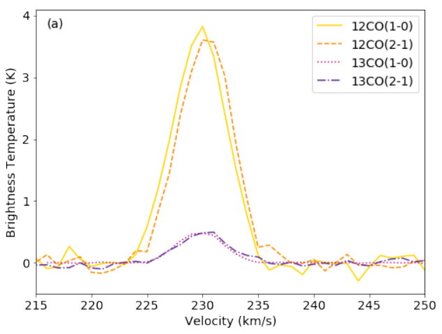
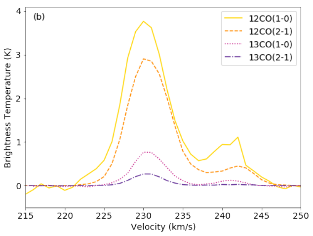
When computing RADEX models, we used a homogeneous spherical escape probability geometry with a line width of 1 km s-1 to match our observations’ velocity channels, and a background temperature of 2.73 K. We also assume that the ratio of 12CO to 13CO () is in the range 50–100 (Nikolic07) and that /.
We limited the ranges of the parameters to be between 2 and 200 K, between and cm-3, and between and cm-2. The ranges of and are evenly spaced in log space, is spaced linearly. When computing the RADEX grid, we also excluded regions of the parameter space where RADEX predictions are less reliable, such as where the optical depth gets very large (), where 12CO becomes overpopulated and the excitation gets inflated (KoeppenKegel80, ,), where any output values become unphysically negative, and where RADEX took more than 999,000 iterations to solve.
For each combination of the three parameters, = (, , ), the resultant model brightness temperatures from RADEX, , and the beam filling factor, , were used to compute a probability given the observed brightness temperature for some voxel, , and its error, , for each observed line, , using the equation
| (1) |
We find the combination of parameter values that yields the greatest probability, . We then find the odds ratio for all other parameter combinations in the grid:
| (2) |
In the case of uniform priors (so , which we assume here for all parameters), this reduces to the Bayes Factor:
| (3) |
To compare with all other combinations of parameters, we use the “Jeffreys” scale (Trotta08) to determine if is “inconclusively”, “weakly”, “moderately”, or “strongly” preferred to the other parameter combinations. Trotta08 defines this empirically derived scale as follows: a value of corresponds to inconclusive evidence, is weak evidence, is moderate evidence, and is strong evidence. The value of is zero for , and increases for parameter combinations that have lower probabilities of matching the observed intensities.
After excluding the regions of parameter space for which ( is strongly preferred over all the excluded parameter combinations) we determine the ranges of the remaining parameter space for each parameter to obtain what we call here “Bayesian intervals”. We do the same to get intervals excluding parameter combinations with and to get intervals outside of which is “moderately” and “weakly” preferred, respectively. In this case, the “strong” 5.0 Bayesian interval is the largest and least constrained of the three since parameter combinations that is only moderately or weakly preferred over are included within the interval. The “weak” 1.0 Bayesian interval is the narrowest and most constrained, since only needs to be weakly preferred over a parameter combination for it to be excluded.
The Bayesian intervals and all depend entirely on the 3-dimensional probability density function (PDF). In addition to these intervals, we also consider each individual parameter’s probability density profile, integrated over the other two parameters. From these profiles, we determine one-sigma and two-sigma, 67% and 95%, confidence intervals, defined as the smallest ranges of the parameters for which the sum under their normalized probability profiles is 0.67 and 0.95, respectively. The confidence intervals depend only on the integrated 1-dimensional profiles instead of the 3-dimensional PDF and therefore depend on the spacing of intervals used in the parameter ranges. Since the and ranges span several orders of magnitude, the confidence intervals are determined in log space so as not to overly weight the higher values. The confidence interval of is calculated with linear spacing.
An example corner plot showing a resultant distribution for one pixel of data is shown in Figure 5. The profiles along the diagonal show some of the metrics described above: , the collapsed 1-dimensional probability profiles, and the two smallest Bayesian intervals.

We attempted to independently constrain in the same way as the other parameters, adding it as a fourth dimension to the tested parameter space. However, was rarely constrained and including it significantly increased the computational requirements. We therefore assumed a range of = 50–100 instead (Nikolic07) and performed the fitting once with = 50 and once with = 100. With additional observations of higher J 12CO and 13CO lines, we might be able to constrain on a pixel-by-pixel basis, making it worth the additional computational requirements.
We similarly attempted to include fitting the beam filling factor as a fourth parameter with minimal success. Appendix goes into detail about the various attempts at fitting and measuring the beam filling factor. After examining the results of these attempts, we used a range of filling factors from 10%–20%. The lower limit of this range comes from unphysical fitting solutions (primarily defined as excessively large line-of-sight path lengths) and the upper limit comes from measured upper limits when comparing the high resolution 13CO(1-0) observations at 13″ to the low resolution maps at 45″. The exception to this is the arcminute region at 5:39:50 -70:08:00, where we found a lower limit on the filling factor to be 15% rather than 10%. A filling factor of 10% results in line-of-sight path lengths that are pc while the radius of the clouds in the region are measured to be pc. We do not take into account any potential difference in beam filling factors between different lines, despite them likely having different spatial distributions.
Using simulated data from the full range of the parameter space based on expected emission from RADEX and the measured rms error in the observed maps, we evaluated how well our data can be fit by the process described here. We also evaluated which of the Bayesian and confidence intervals best recovered true parameter values while still constraining their values. The full evaluation process is described in Appendix and additional related plots are available as supplementary material44 4 https://doi.org/10.5281/zenodo.4646288. The true parameter values were almost always recovered at cm-2 and for the full range of and . The intervals that were determined to best characterize the true parameter values were a combination of the 95% confidence interval and the 1.0 Bayesian interval. They showed similarly high recovery rates of the true parameter values and had the tightest constraints on those values. In some regions the 95% confidence interval was better constrained than the 1.0 Bayesian interval, and vice versa, hence the combination of the two.
We also consider how the fitting process depends on including all four observed lines–12CO(1-0), 13CO(1-0), 12CO(2-1), 13CO(2-1)–and how it would change if we included only the three lines with the best angular resolution and dropped 12CO(1-0), which has a resolution of 45″. This would allow us to do the entire fitting process at higher resolution since we would instead be limited by the 13CO(2-1) at 30″. We consider this case in Appendix using the fitting evaluation methods described in Appendix . We find that dropping the 12CO(1-0) results in a loss of sensitivity to moderate values of . While the resulting fitted intervals still include the correct value almost all the time for cm-2, they are only well-constrained for cm-2. We decided that the improvement in resolution is not worth the loss in sensitivity to this range of column densities.
III.2 Generating Maps of Physical Parameters


We perform the RADEX fitting on each of the pixels in the map. For each velocity component within each pixel, we find the peak of the 13CO(1-0) line profile for a single velocity component and perform a full fit of the three physical parameters—, , —for the peak value. We then assume that and are constant for that line of sight and fit the rest of the line only considering the and that were in the fitted interval of the line peak to get across the line. We include only velocities for which at least two lines have detections above 5. is then summed over the line to get a total value for the pixel. Upper and lower errors come from the upper and lower bounds of the fitted interval for each parameter, and for , the upper errors and lower errors are propagated separately to get upper and lower errors on the total for the line.
We also considered two other methods for this fitting process: fitting all three parameters for each voxel along the line of sight or holding and fixed for the entire cloud after segmenting the emission into clumps. These alternative methods are compared in Appendix , where we find that the method described here of holding and fixed for the line of sight yielded the most reliable realistic results.
This process was done once with =50 and once with =100, and also once each with a filling factor of 10% and 20% for a total of four runs, with the exception of the region around 5:39:50 -70:08:00, for which we used a lower limit on the filling factor of 15% rather than 10% as described in Appendix . To correct our final results for this filling factor, we multiplied the fitted by the assumed filling factor for the clump. We did not correct the values for the filling factor, so the values reported are those of clump structures on the scale of the assumed filling factor (4.5″ 6.75″ or 9″ for filling factor of 10%, 15%, or 20%, respectively).
When approaching a boundary between two velocity components, both spatially and in velocity space, we drew a hard barrier rather than doing any partial pixel assignments to account for overlapping line wings or spatial overlap. To check if this affected the fitting results, we did the RADEX fitting for three overlapping velocity components, but this time fitting Gaussian line profiles to each pixel to appropriately assign partial emission to the overlapping clumps. The RADEX fitting code used this partial emission assignment and continued the fitting as before. This did not result in any significant change in any of the derived quantities, and so fortunately the detailed accounting of multiple velocity components does not need to be added in general to this kind of analysis. This is likely because the line wing that was cut from Component A and assigned to Component B is well accounted for by the line wing of Component B that was assigned to Component A, so the amount of emission is not significantly changed. This result might change if there is a large temperature difference between overlapping components, but that seems unlikely to occur in most scenarios.
The results for each velocity component were combined into maps of the whole Ridge shown in Figure 6 by adding along each line of sight and using a mass-weighted average for and . We masked fits that were not well-constrained since our results from Appendix showed that poorly constrained fits often were also not accurate. How well each parameter could be expected to be constrained varied largely, as shown in Appendix . and were both usually tightly constrained, while the fitted is not as well constrained. This appears to be a reflection of how well the data at hand can inform the physical parameters rather than a reflection of how reliable the fitting process is. For both Figure 6 and deriving quantities in §, we masked values of where the error was more than 80%, where the error was more than 50%, and where the error was more than 200%. We also masked values of that were less than 3 K, and values of that rose sharply at the edges of clumps. In the case of the Molecular Ridge, we accomplished this by masking where was greater than 104 cm-3 since values larger than that only occurred in edge pixels, but this would change if the range of fitted had been higher.
After cutting pixels that had poorly constrained or unphysical fits, we combined fitted values from the runs with different and filling factors. The reported values for , , and are the mean of the best fit values from the =50 and =100 results and the 10% and 20% filling factor results. The upper and lower errors are from the highest and lowest values included in any of the fitted intervals (i.e. if is K for =50 and K for =100, the reported is K). When reporting a single error, we use the geometric mean of the upper and lower error. This results in the maps shown in Figure 6 sometimes having larger errors than the cutoffs described here.
IV Clump Definitions and Properties
IV.1 Clump Definitions

We used quickclump55 5 https://github.com/vojtech-sidorin/quickclump/(Sidorin17), which is a Python clump-finding algorithm that is similar in methodology to clumpfind (clumpfind) and DENDROFIND (Wunsch12). These clumps are based on the ALMA 13CO(1-0) cube convolved to 45″ to match the lowest resolution observation (the 12CO(1-0) from MAGMA), and the input parameters used were Nlevels=1000, Tcutoff=4=1.4 K, dTleaf=4=1.4 K, and Npixmin=5. A map of the 32 clumps identified by quickclump is shown in Figure 7 where they are also given identifying numbers. Each voxel in the data cube was assigned to at most a single clump, so overlapping clump borders in Figure 7 indicate that the clumps overlap along the line of sight and are differentiated by their velocity structure. The integrated line fluxes for each of these clumps and each observed line are given in Table . Clumps 3, 10, and 11 do not have corresponding APEX data and so were not included in the RADEX fitting.
If any clump had more than 75% of the pixels masked in any parameter, we removed the entire clump from the following analysis; this was only the case for in clumps 1, 20, 29, 30, and 32. We also discarded the fits of clumps 9, 15, and 21 because they had very few pixels with successful fits, the fitted parameters had large variations from pixel-to-pixel, and they were major outliers in later trends.
[tabular=l|c|c|c|c|c,
table head=Clump 12CO(1-0) 12CO(2-1) 13CO(1-0) 13CO(2-1) CS(2-1)
]
LineStrengthTable.csv
ClumpNames=\name,W12CO10=\wco, W13CO10=\wtco, W12CO21=\wcot, W13CO21=\wtcot, WCS21=\wcs, W12CO10err=\ewco, W13CO10err=\ewtco, W12CO21err=\ewcot, W13CO21err=\ewtcot, WCS21err=\ewcs, test=\test
\name \wco\ewco