Cell fusion through slime mold network dynamics

Sheryl Hsu^a and Laura P. Schaposnik^⋆,b Affiliation: (

\star

) Corresponding author: schapos@uic.edu

Abstract

Physarum Polycephalum is a unicellular slime mold that has been intensely studied due to its ability to solve mazes, find shortest paths, generate Steiner trees, share knowledge, remember past events, and the implied applications to unconventional computing. The CELL model is a unicellular automaton introduced in plu8 that models Physarum’s amoeboid motion, tentacle formation, maze solving, and network creation. In the present paper, we extend the CELL model by spawning multiple CELLs, allowing us to understand the interactions between multiple cells, and in particular, their mobility, merge speed, and cytoplasm mixing. We conclude the paper with some notes about applications of our work to modeling the rise of present day civilization from the early nomadic humans and the spread of trends and information around the world. Our study of the interactions of this unicellular organism should further the understanding of how Physarum Polycephalum communicates and shares information.

Keywords:

Cell fusion, network dynamics, slime mold

I Introduction

Physarum Polycephalum is a unicellular slime mold. At one point in its life cycle, it forms a plasmodium with many tubes. Experiments have shown that Physarum Polycephalum in this plasmodium state is able to solve mazes, find the shortest path, build high-quality networks between multiple points, adapt and respond to stimulus, and also remember past events plu14; plu15; plu16. Recently, several mathematical models inspired by Physarum have been developed to approach problems such as the shortest path or Steiner tree problems plu8; plu12; plu6; april2.

The behavior of Physarum Polycephalum can be studied, in particular, using cellular automaton as done in plu8 through what the authors called the CELL model. In this model, a Physarum cell is modeled on a grid with cytoplasm and cytoskeleton. At each iteration, the cytoplasm and cytoskeleton is slightly reshaped with the introduction of an outside bubble. As shown in plu8, this model can be used to simulate ameboid motion with tentacle formation, maze solving, shortest path finding, and network creation.

Inspired by plu8, we take a novel approach which allows us to discern several interesting patterns. When considering cells, one expects to observe certain behaviors. In particular:

(a)

The time it takes for two cells to merge should increase directly with the distance between them.
(b)

It should be fastest and most likely for cells to merge with the cell closest to them.
(c)

The smaller a cell is, the more mobile it should be.
(d)

The smaller cells are, the better they should fuse in terms of cytoplasm mixing.

We shall begin this paper by introducing in Section II some of the different models used in the literature to study Physarum Polycephalum, paying particular attention to the flow-conductivity model plu6, the cellular model plu8, the multi-agent model plu12, and the shuttle-streaming model april2.

After introducing these models, we dedicate Section III to the main findings of our work. By considering cells at different distances apart and studying the number of iterations it took for them to merge, we could see that:

•

The relationship between distance and iterations is linear, as shown in Figure 14.

By considering three cells and adjusting the distance between them, we measured which cells merge first and the number of iterations it took them to do so, allowing us to see that:

•

The two closest cells are most likely to merge together, followed by the next two closest cells, followed by the two furthest cells;
•

The two closest cells take the least number of iterations to merge, followed by the next two closest cells, followed by the two furthest cells.

We also considered cells of different sizes and measure mobility using the average distance from spawn point, maximum distance from spawn point, and speed, leading to the following results:

•

The relationship between average distance and size is exponentially decreasing;
•

The relationship between maximum distance and size is exponentially decreasing;
•

The relationship between speed and size is also exponentially decreasing.

Finally, by considering the fusion of two cells of varying sizes, we measured cytoplasm mixing using Lacy’s mixing index plu13, leading to the following findings:

•

There is a decreasing exponential relationship between the mean mixing index and cell area;
•

There is a decreasing logistical relationship between max mixing index and cell size.

We conclude this paper expanding on the analysis and applications of the above findings in Section IV. In particular, we explore the applications of our work to modeling the rise of present day civilization from the early nomadic humans and the spread of trends and information around the world.

II Modelling Physarum Polycephalum

We shall dedicate this section to reviewing four models inspired by Physarum Polycephalum, and which we shall consider in the present paper when building a new model to study cell fusion between multiple cells. We shall begin by reviewing a flow-conductivity model in Section II.1, a cellular model in Section II.2, and a multi-agent model in Section II.3. Finally, we shall conclude the section by introducing a shuttle-streaming model in Section II.4. A good overview of current literature on Physarum Polycephalum can be found at plu3.

II.1 Flow-conductivity model

Inspired by the idea that within Physarum Polycephalum tubes of the plasmodium grow thicker as more protoplasm flows through that tube, the authors of plu6 introduced a flow-conductivity model which we shall review below. In this setting, two further observations about Physarum’s behavior come into play:

•

when two tubes connect to the same food source, the longer one usually disappears;
•

open-ended tubes are likely to disappear.

In what follows, we shall describe this model following the ideas of plu6. Consider nodes $N_{1},N_{2}\dots$ , and let $N_{1}$ be the source node (start) and $N_{2}$ be the sink node (end). The tube/edge connecting nodes $N_{i}$ and $N_{j}$ , is denoted as $M_{ij}$ . Let $Q_{ij}$ be the flux through $M_{ij}$ , let $p_{i}$ be the pressure at node $i$ , let $L_{ij}$ be the length of $M_{ij}$ , and let $D_{ij}$ be the conductivity of $M_{ij}$ . Then, we have

Q_{ij}=\frac{D_{ij}}{L_{ij}}(p_{i}-p_{j}).

(1)

By Kirchhoff’s law,

\displaystyle\sum_{i}Q_{ij}=0\quad(j\neq 1,2).

(2)

Since $N_{1}$ and $N_{2}$ are the start and end node respectively,

	$\displaystyle\sum_{i}Q_{i1}+I_{0}$	$\displaystyle=$	$\displaystyle 0;$		(3)
	$\displaystyle\sum_{i}Q_{i2}-I_{0}$	$\displaystyle=$	$\displaystyle 0.$		(4)

The adaptation of the tube thickness can be modeled using the following equation:

\frac{d}{dt}D_{ij}=f(|Q_{ij}|)-rD_{ij},

(5)

where $f(Q)$ must be an increasing function with $f(0)=0$ , and thus for the purposes of this model one may consider $f(Q)=\alpha|Q|$ . Setting $p_{2}=0$ , one can compute all the $p_{i}^{\prime}s$ using equations (2)-(4) and therefore all $Q_{ij}$ . The flow-conductivity model has been used to find Steiner trees6684158, solve the traveling salesman problem 10.1007/978-3-642-38703-6_35, and design fault-tolerant networks FaultTolerant. It has been applied to creating a shortest path navigation system across the US interstate highway plu6, designing railroad networks similar to the Tokyo railroad system Tero439, designing transportation networks with changing traffic distributions 10.1371/journal.pone.0089231, identifying focal nodes for disease spread in epidemiological networks disease, and solving supply chain network design problems doi:10.1080/00207543.2016.1203075.

Example 1.

In order to illustrate how the flow-conductivity model can be used, consider the graph in Figure 1, where 1 is the source node and 6 is the sink node.

Refer to caption — Figure 1: Node 1 is the source node and node 6 is the sink node. The number on each edge represents the length of that edge.

Starting with a flux of $I_{0}=10$ into node 1, and assuming all tubes start off with the same conductivity $D_{ij}=2$ , one has the following system of equations:

$\displaystyle\frac{2}{2}(p_{2}-p_{1})+10$	$\displaystyle=$	$\displaystyle 0$
$\displaystyle\frac{2}{2}(p_{1}-p_{2})+\frac{2}{3}(p_{3}-p_{2})+\frac{2}{7}(p_{4}-p_{2})$	$\displaystyle=$	$\displaystyle 0$
$\displaystyle\frac{2}{3}(p_{2}-p_{3})+\frac{2}{5}(p_{4}-p_{3})+\frac{2}{4}(p_{5}-p_{3})$	$\displaystyle=$	$\displaystyle 0$
$\displaystyle\frac{2}{7}(p_{2}-p_{4})+\frac{2}{5}(p_{3}-p_{4})+\frac{2}{1}(p_{5}-p_{4})$	$\displaystyle=$	$\displaystyle 0$
$\displaystyle\frac{2}{4}(p_{3}-p_{5})+\frac{2}{1}(p_{4}-p_{5})+\frac{2}{6}(p_{6}-p_{5})$	$\displaystyle=$	$\displaystyle 0$
$\displaystyle\frac{2}{6}(p_{5}-p_{6})-10$	$\displaystyle=$	$\displaystyle 0.$

Setting $p_{6}=0$ and solving this system, leads to the values $p_{1}=57;$ $p_{2}=47;$ $p_{3}=38;$ $p_{4}=33;$ and $p_{5}=30.$ Then, from Eq. (1) one has $Q_{12}=10;$ $Q_{23}=6;$ $Q_{24}=4;$ $Q_{34}=2;$ $Q_{35}=4;$ $Q_{45}=6;$ and $Q_{56}=10.$ Updating $D_{ij}$ using $\Delta D_{ij}=\alpha|Q_{ij}|-rD_{ij}$ , and taking $\alpha=1$ , and $r=1$ one has that

	$\displaystyle\Delta D_{12}$	$\displaystyle=$	$\displaystyle 8;~\Delta D_{23}=4;~\Delta D_{24}=2,$
	$\displaystyle\Delta D_{34}$	$\displaystyle=$	$\displaystyle 0;~\Delta D_{35}=2;~\Delta D_{45}=4;~\Delta_{56}=8.$

The updated values of $D_{ij}$ then are:

	$\displaystyle D_{12}=10;~D_{23}=6;~D_{24}=4,$
	$\displaystyle D_{34}=2;~D_{35}=4;~D_{45}=6;~D_{56}=10.$

After repeating this process several times, a path appears when a lot of the $D_{ij}$ are close to zero and then the rest are much greater.

II.2 Cellular model

In the cellular model as described in plu8, or CELL model, a cell is a mass of cytoplasm surrounded by a membrane, which is placed on a lattice grid where every square has an assigned number/state. State 2 represents cytoskeleton, state 1 represents cytoplasm, and state 0 represents squares that are not part of the CELL. The model is based on the following assumptions:

1.

The membrane is the part of the cell where the cytoskeleton is concentrated and hardened;
2.

When a cytoskeleton assembly is taken apart and the membrane softens, the cytoplasm is distributed to other areas of the cell;
3.

Cytoplasmic flow is accompanied by transportation of the cytoskeleton and distribution of cytoskeleton assemblies.

The CELL model has two phases: development and foraging. In the development phase, the cell grows, forming a diamond shaped model with cytoskeleton around the edges and cytoplasm inside. In the foraging stage, the model “eats” zero which leads to a redistribution of cytoplasm and cytoskeleton/membrane. The algorithm is as follows:

1.

Chose a site with state 2, the stimulus point;
2.

Randomly choose a neighbor of the stimulus point in state 0 and replace the state of the stimulus point with the state of the chosen neighbor, so zero invades the cell. We call the zero a bubble;
3.

Replace state 1 with 2 so all non-zero cells are 2. Set number of moves to zero;
4.

Mark the site with the bubble;
5.

Decide whether $s$ sites of the bubble’s neighbors are in state 0 or not. If yes, go to 8 otherwise go to 6;
6.

Decide whether the number of moves exceeds threshold $n$ . If yes, go to 8 otherwise go to 7;
7.

Randomly choose one of the bubble’s non-marked neighbors which is in state 2. Replace the state of the bubble with the state of chosen neighbor. Add 1 to number of moves, go to 4;
8.

Reorganize the boundary and inside using algorithm described above. For example, if site with state 2 is surrounded by only neighbors with state 2, its state is changed to 1. Return to 1.

It should be noted that depending on the location of the stimulation, the model behaves differently. If the stimulus point is chosen randomly, the CELL moves like an amoeba. If the stimulus is chosen from several active zones, an adaptive network with tentacles forms.

Example 2.

In order to illustrate the model, we shall consider the CELL model in a $5\times 5$ grid. After the initial growth stage, the CELL model is seen in Figure 2 (a) below. By randomly choosing a cell (seen in grey) to be the stimulus point, and choosing a neighbor and swapping, one can see the following step in Figure 2 (b):

In the following steps, one has the bubble randomly swap with neighbors more times. Doing this a couple more times one obtains Figure 3 (a). Finally, one can reassign states to the cells, leading to Figure 3 (b).

A typical CELL has bubbles within its cytoplasm. If enough of these bubbles group together, a chamber can form within the CELL. When this chamber bursts, tentacles are formed, as illustrated in Figure 4.

This model can also be used to form networks and find the shortest path. This is mainly done by creating active zones in which the stimulus point is always chosen from. For example, in Figure 5, active zones are created in three regions of the cell, leading to the cell forming a tree between the three active zones. Finally, this model has been previously used to solve mazes, generate spanning trees plu8, and model crowd evacuation april1.

II.3 Multi-agent model

Inspired by the many different behaviors Physarum demonstrates, the authors of plu12 introduced a multi-agent model which consists of agents who travel throughout Physarum, forming a chemoattractant map. We shall represent this as a large grid similar to the CELL model, and consider an agent to fill a cell of the grid. Each agent also has three sensors which sample values sensor offset distance (SO) away. The agents then uses the readings from the three sensors and orient themselves towards the strongest chemoattractant reading from the sensors.

There are two important parameters which need to be considered in this set up:

•

There is sensor angle (SA), which is the angle between two of the three sensors;
•

There is the rotation angle (RA) which is the amount the agent rotates to the strongest chemoattractant reading.

For example, if RA $<$ SA, contraction behavior is increased but if RA $>$ SA, spontaneous branching happens.

The agent first reads from each of its 3 sensors. It turns by RA in the direction of the greatest sensor. After the agent has rotated accordingly, the agent attempts to move forward. If it can move forward (the cell isn’t occupied), chemoattractant is deposited ( and the grid is updated) and then move. Agents are randomly chosen to rotate and then move. In addition, a $3\times 3$ mean filter is applied on the grid to simulate diffusion. Depending on where one initializes agents, and what the SA and RA are, one gets different behaviors for the system, which can be summarized as follows:

•

Filamentous condensation method. Initialize a few agents at random locations and orientations. Then, a network forms. Add food sources which emit chemoattractants and the network will form a Steiner tree.
•

Filamentous Foraging Method. Initialize agents at food sources.
•

Plasmodial Shrinkage Method. Randomly remove agents, other agents will move and form a minimum spanning tree.

Example 3.

To understand the multi agent model described above, we shall consider the following chemoattractant map shown in Figure 6 (a), and assume one has an agent with $SA$ , and $RA=45$ at the shaded square in Figure 6 (a). The rightmost sensor will then sense the highest chemoattractant (29) and the agent will rotate 45 degrees to the right. The sensor then moves forward if possible and deposits chemoattractant on the map (we shall assume it always deposits 5), and thus the next step in the model can be seen in Figure 6 (b) below.

To simulate diffusion, we then apply a $3\times 3$ mean filter to the map where we replace the value of each cell with the average of the cells in the $3\times 3$ surrounding box, leading to the following Figure 7.

Finally, it should be noted that through this model one can see the agents gradually move from being randomly distributed to forming a network, as shown in Figure 8.

II.4 Shuttle-streaming model

We shall next describe the shuttle-streaming model following april2. This model is based on three biological observations about Physarum polycephalum:

•

open ended tubes gradually disappear;
•

when two tubes connect the same food sources, the longer one disappears;
•

outside changes like addition of nutrients can cause changes to the rhythmic contractions and shuttle streaming of Physarum.

Shuttle streaming is the flow of protoplasm through Physarum’s tubes and plays an important role in chemical signalling. When the organism contracts periodically (1-3 min), the direction of the shuttle streaming changes as hydrostatic pressure is produced.

In order to find the shortest path from node $v_{S}$ to $v_{F}$ , which are two food sources, one considers two different protoplasmic flows, originating at each of the two nodes $v_{S},$ and $v_{F}$ .

Forward flow ( $v_{S}$ to $v_{F}$ ). The amount ${\rm Re}_{f}((v_{i},v_{j}),t)$ of nutrients received from node $v_{i}$ through edge $(v_{i},v_{j})$ during forward flow is given by

{\rm Re}_{f}((v_{i},v_{j}),t)={\rm Se}_{f}((v_{i},v_{j}),t)-\eta L_{ij},

(6)

where ${\rm Se}((v_{i},v_{j}),t)$ is the amount of nutrients sent through edge $(v_{i},v_{j})$ at node $v_{i},$ the value $L_{ij}$ is length of edge, and $\eta$ is the absorption rate per unit length of tube wall. Additionally, ${\rm totRe}(v_{j},t)$ is the total amount of nutrients that node $v_{j}$ receives.

The node $v_{j}$ distributes the total amount of nutrients received in forward flow proportionally to the amount received in previous backward flow. Hence, the amount of nutrients sent out through edge $(v_{j},v_{k})$ by node $v_{j}$ is given by

$\displaystyle{\rm Se}_{f}((v_{j},v_{k}),t)$	$\displaystyle=$	$\displaystyle{\rm totRe}_{f}(v_{j},t)\times\frac{{\rm Re}_{b}((v_{k},v_{j}),t-\delta t)}{{\rm totRe}_{b}(v_{j},t-\delta t)}$
$\displaystyle{\rm totRe}_{f}(v_{j},t)v$	$\displaystyle=$	$\displaystyle\sum_{\forall v_{i}\in(v_{i},v_{j})}{\rm Re}_{f}((v_{i},v_{j}),t)$
$\displaystyle{\rm totRe}_{b}(v_{j},t-\delta t)$	$\displaystyle=$	$\displaystyle\sum_{\forall v_{k}\in(v_{k},v_{j})}{\rm Re}_{b}((v_{k},v_{j}),t-\delta t)$

Backwards flow at time $t+\delta t$ . Similar to the forward flow, one has that

{\rm Re}_{b}((v_{p},v_{q}),t+\delta t)={\rm Se}_{b}((v_{p},v_{q}),t+\delta t)-\eta L_{pq}.

The corresponding equations for

\displaystyle\phi:=\frac{{\rm Re}_{f}((v_{r},v_{q}),t)}{{\rm totRe}_{f}(v_{q},t)}

are given by

$\displaystyle{\rm Se}_{b}((v_{q},v_{r}),t+\delta t)$	$\displaystyle=$	$\displaystyle{\rm totRe}_{b}(v_{q},t+\delta t)\times\phi;$
$\displaystyle{\rm totRe}_{b}(v_{q},t+\delta t)$	$\displaystyle=$	$\displaystyle\sum_{\forall v_{p}\in(v_{p},v_{q})}{\rm Re}_{b}((v_{p},v_{q}),t+\delta t);$
$\displaystyle{\rm totRe}_{f}(v_{q},t)$	$\displaystyle=$	$\displaystyle\sum_{\forall v_{r}\in(v_{r},v_{q})}{\rm Re}_{f}((v_{r},v_{q}),t).$

The two nodes $v_{S}$ and $v_{F}$ act as both source and sink nodes depending on the direction of the protoplasmic flow. Assuming that the amount of nutrients the tubular network absorbs per one forward or backward flow session is $N_{in}$ , the amount of nutrients sent and received by nodes $v_{s},v_{F}$ can be computed in the following fashion.

At $t=0$ one can compute the number of nutrients sent from node $v_{j}$ as follows:

{\rm Se}_{f}((v_{j},v_{k}),T=0)=\frac{{\rm totRe}_{f}(v_{j},t=0)}{\sum\limits_{\forall v_{k}\in(v_{j},v_{k})}1}

(7)

This can be thought of as the total amount of nutrients divided by the number of edges. When the nutrients carried by an edge is zero or negative, we can discard the edge since biologically it would die without nutrients. One continues to do this until the end of the optimization process is reached, at which point each node only has one in-edge and one out-edge.

Example 4.

To illustrate this model, consider a similar graph to the flow-conductivity model of Figure 1:

Let $N_{in}=10$ , which means one puts in 10 nutrients every time. The starting values can be then computed using Equation (7). Let $\eta=0.1$ . Then we have that

$\displaystyle{\rm Se}_{f}((1,2),0)$	$\displaystyle=$	$\displaystyle 10,$
$\displaystyle{\rm Re}_{f}((1,2),0)$	$\displaystyle=$	$\displaystyle 9.8,$
$\displaystyle{\rm Se}_{f}((2,3),0)$	$\displaystyle=$	$\displaystyle 4.9,$
$\displaystyle{\rm Re}_{f}((2,3),0)$	$\displaystyle=$	$\displaystyle 4.6,$
$\displaystyle{\rm Se}_{f}((2,4),0)$	$\displaystyle=$	$\displaystyle 4.9,$
$\displaystyle{\rm Re}_{f}((2,4),0)$	$\displaystyle=$	$\displaystyle 4.2,$
$\displaystyle{\rm Se}_{f}((3,5),0)$	$\displaystyle=$	$\displaystyle 4.6,$
$\displaystyle{\rm Re}_{f}((3,5),0)$	$\displaystyle=$	$\displaystyle 4.2,$
$\displaystyle{\rm Se}_{f}((4,5),0)$	$\displaystyle=$	$\displaystyle 4.2,$
$\displaystyle{\rm Re}_{f}((4,5),0)$	$\displaystyle=$	$\displaystyle 4.1,$
$\displaystyle{\rm Se}_{f}((5,6),0)$	$\displaystyle=$	$\displaystyle 8.3,$
$\displaystyle{\rm Re}_{f}(5,6)$	$\displaystyle=$	$\displaystyle 7.7.$

The values of ${\rm totRe}_{f}(v,0)$ can be computed in a similar manner, and are given by

$\displaystyle{\rm totRe}_{f}(1,0)$	$\displaystyle=$	$\displaystyle 10,$
$\displaystyle{\rm totRe}_{f}(2,0)$	$\displaystyle=$	$\displaystyle 9.8,$
$\displaystyle{\rm totRe}_{f}(3,0)$	$\displaystyle=$	$\displaystyle 4.6,$
$\displaystyle{\rm totRe}_{f}(4,0)$	$\displaystyle=$	$\displaystyle 4.2,$
$\displaystyle{\rm totRe}_{f}(5,0)$	$\displaystyle=$	$\displaystyle 8.3,$
$\displaystyle{\rm totRe}_{f}(6,0)$	$\displaystyle=$	$\displaystyle 7.7.$

Now it is time for backwards flow. Starting from the opposite end, one sets ${\rm Se}_{b}((6,5),1)=10$ , and so ${\rm Re}_{b}((6,5),1)=9.4.$ Then, one has that

$\displaystyle{\rm Se}_{b}((5,3),1)$	$\displaystyle=$	$\displaystyle 4.7566267,$
$\displaystyle{\rm Re}_{b}((5,3),1)$	$\displaystyle=$	$\displaystyle 4.3566267,$
$\displaystyle{\rm Se}_{b}((5,4),1)$	$\displaystyle=$	$\displaystyle 4.64337,$
$\displaystyle,{\rm Re}_{b}((5,4),1)$	$\displaystyle=$	$\displaystyle 4.54337,$
$\displaystyle{\rm Se}_{b}((3,2),1)$	$\displaystyle=$	$\displaystyle 4.3566267,$
$\displaystyle{\rm Re}_{b}((3,2),1)$	$\displaystyle=$	$\displaystyle 4.0566267,$
$\displaystyle{\rm Se}_{b}((4,2),1)$	$\displaystyle=$	$\displaystyle 4.54337,$
$\displaystyle{\rm Re}_{b}((4,2),1)$	$\displaystyle=$	$\displaystyle 3.84337,$
$\displaystyle{\rm Se}_{b}((2,1),1)$	$\displaystyle=$	$\displaystyle 7.9,$
$\displaystyle{\rm Re}_{b}((2,1),1)$	$\displaystyle=$	$\displaystyle 7.7.$

As done with forward flow, one can compute ${\rm totRe}_{b}$ and then repeat the same procedure with forward flow. After repeating the procedure several times, the flow through certain edges will eventually become very small at which point one can remove such edges until obtaining the shortest path.

Since the model is a shortest path algorithm, it can be thought of as being very similar to flow-conductivity, so any of the shortest path applications such as traffic routing should be possible, although this model has been shown to not always give the shortest path.

III Exploring interactions between multiple cells

In what follows we shall introduce a modified version of the CELL model described theoretically in plu8 with memorized flow. After creating code to model our new algorithm, we shall investigate the interactions between multiple cells. To do this, our new model incorporates a unique ID corresponding to a color for each cell, so that each cell is spawned with a unique color, allowing us to distinguish between the cytoplasm of each cell.

Example 5.

An example of our model is shown in Figure 10, where one can see two CELLs initially spawned in a diamond shape. After a few iterations, one can see the cells lose their diamond shape and become more circular, and there are multiple chambers within the cells.

By the third image of Figure 10, the cells have made contact. In the fourth image, cytoplasm continues to flow between the two newly connected cells. In the fifth and sixth image, cytoplasm continues to flow further between the two cells. Finally in the seventh image, the cytoplasm appears to start becoming well mixed and in the eight image, the cell seems to have taken on a more circular or compact shape after initially being elongated due to two cells combining. In the ninth image, the cell seems circular and the cytoplasm is well dispersed. In the following sections we shall see further analysis of how cells fuse through our model.

III.1 Time to cell fusion in relation to spawn distance

We shall dedicate this section to understanding how the distance two CELLs are spawned apart affects the number of iterations it takes for the cells to contact. Across the section, we use the following parameters: n = 1000, s = 3, and define two CELLs contacting as a cytoplasm of one ID being adjacent to a cytoplasm of another CELL. To illustrate this definition, Figure 11 is an example of the first place two CELLs contact.

Figure 11: In this image, the two cells have just contacted for the first time.

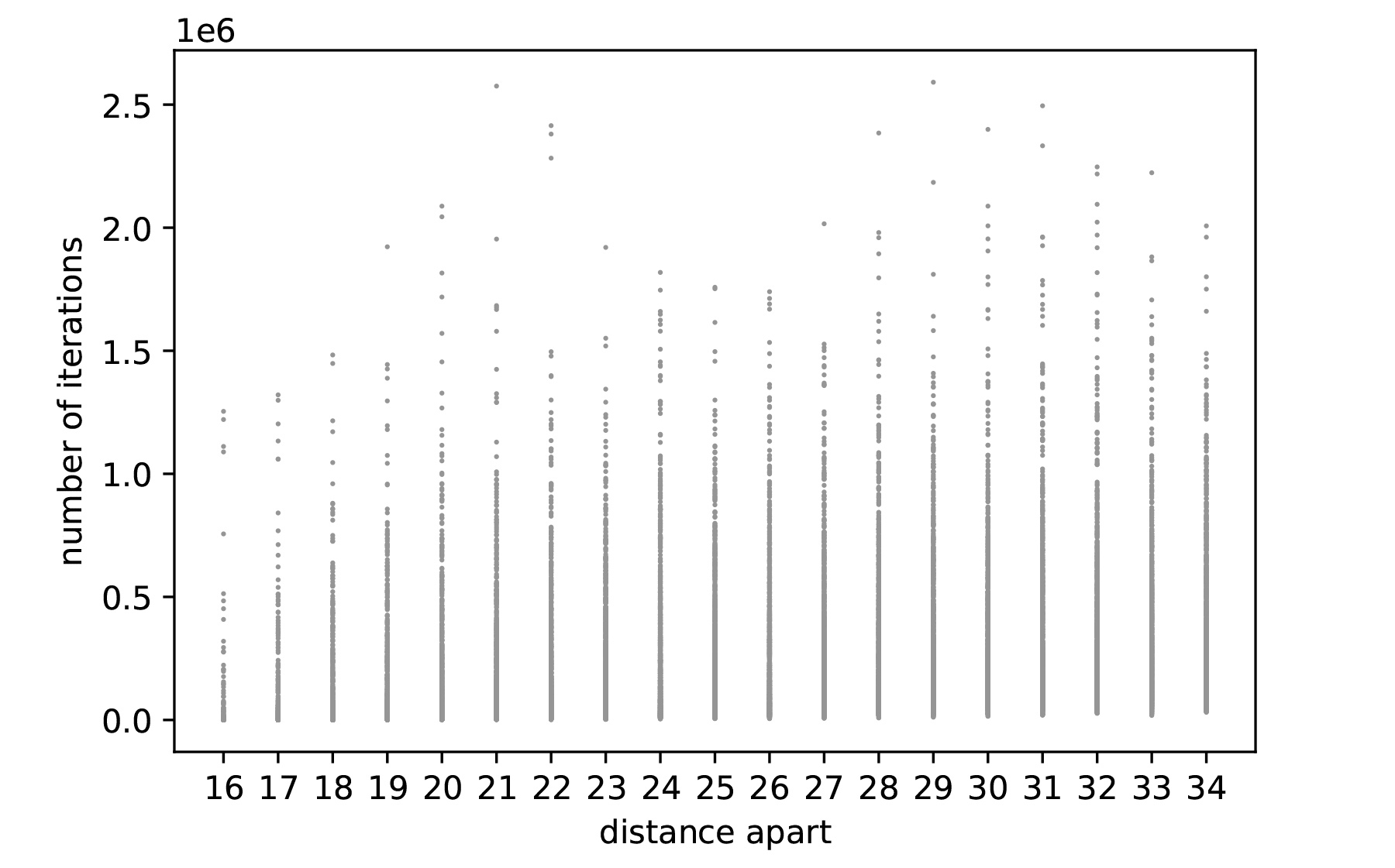
To understand the behavior of two cells through our model, we run 1025 trials of each spawn distances from 16 to 34. We graph the average iterations of each trial versus the spawn distance in Figures 12 and 13. These plots shows that there are extreme upper outlines, which is expected given the random nature of the cell model. The boxplot also shows an overall increasing trend in number of iterations as the spawn distance increases.

In order to understand the results inferred from our experiments, we fit our findings to curves to linear, exponential, and logistical functions:

$\displaystyle y$	$\displaystyle=$	$\displaystyle mx+b$	(8)
$\displaystyle y$	$\displaystyle=$	$\displaystyle a\cdot b^{x}+c$	(9)
$\displaystyle y$	$\displaystyle=$	$\displaystyle\frac{L}{1+e^{-k(x-x_{0})}}+b.$	(10)

The 10 percent trimmed mean of each spawn distance is given in Figure 14, where one can see that this data appears to be linear (Eq. (8)) with values of $m=18873.73644734$ and $b=-291495.3914131$ . It can be seen that the linear function gives an $r^{2}$ value of $0.9707$ and appears to fit the data, allowing us to conclude that the relationship between time to merge and the distance apart is linear.

Figure 14: To deal with the heavily skewed data as evidenced by the scatter and box plots, we trim 10 percent from both the upper and lower ends of the data. We then compute the trimmed mean. We use the scipy.optimize.curve_fit function to fit this data to a linear function (Eq. (8)) with the values

m=21892.74674907

and

b=-354967.6942326

. This gives a

r^{2}

value of

0.970675948980436

III.2 Analysis of cell fusion with three cells

The premise of this experiment is that we spawn three CELLs in a straight line. We adjust the distances between the cells in order to see which cells fuse first as well as gather data on the number of iterations taken for the first cell fusion event to occur. We try different distances between the three CELLs ranging from 16 to 29 inclusive. We keep track of how many iterations it takes for the first two CELLs to merge and which two cells end up merging. We perform 350 trials. In general, the distance between cells 1 and 2, or distance 1, will be greater than or equal to the distance between cells 2 and 3, or distance 2. We always spawn cell 2 in the center of the image and then spawn cells 1 and 3 the set distance away from cell 2. For example, in Figure 15, the cells are from left to right 1, 2, and 3.

Figure 15: Three cells of size 15, labeled from left to right as 1, 2, and 3. The distance between cells 1 and 2 (distance 1) is 27 and between cells 2 and 3 (distance 2) is 23.

In order to visualize the data from our experiments, we use a a 3D scatterplot in Figure 16, through which we see that there are extreme outlines when both distances are very large.

Moreover, one can see that for every set of distances, there are 3 different possibilities: cells 1 and 2 join, cells 2 and 3 join, or cells 1 and 3 join. For each of these possibilities, we compute the mean number of iterations it took for the cells to fuse. This is displayed in Figure 17. One sees that as the distances increase, so does the number of iterations. In general, it appears that the number of iterations for cells 1 and 3 (green bar) to join is overall much larger than the number of iterations for 1 and 2 or 2 and 3.

Figure 17: Using the python package matplotlib, we compute the mean of each set of distances. For each distance, we have three bars: 1 for each of the possible two CELLs combining.

In order to understand how and when two cells fuse together, we compute the probability that a certain two cells will join, depicted in Figure 18. Overall, one sees that the probability cells 1 and 3 join is the lowest, which is expected since cell 2 is between cells 1 and 3. Cells 2 and 3 have the highest probability of joining which is consistent with the fact that they are closer.

Figure 18: Using the python package matplotlib, we compute the probability that for a given set of distances between CELLs, each combination of two cells (1 2, 1 3, 2 3) will be the ones that combine first.

The number of iterations it takes for two out of the three cells to fuse steeply increases as the distance between the cells does, and this is shown in Figure 19. It is important to note that distance 1 was always greater than distance 2, so the upper triangle of this plot had no data.

III.3 The impact of cell size on movement

In what follows we shall show the importance of the CELL’s size in its ability to move. In this section, we measure mobility by computing three values: the average distance from the spawn point, the furthest distance from the spawn point, and the total distance traveled. After every iteration of the cell algorithm, we compute the center of mass of the cell by iterating through all pieces of cytoplasm and computing the average $x$ and $y$ values. We then compute the distance from the spawn point using the distance formula with the cell’s current center of mass and the spawn point (49, 49). Finally, we compute the total distance traveled by summing the distance between the current center of mass and the center of mass an iteration before. For each calculation, we have 2000 trials of each cell size.

We shall begin by analyzing the average distance from the spawn point. To do this, we compute the ten percent trimmed mean of the average distance for each given cell size, and then fit an exponential curve to this data. The results are shown in Figure 20. The exponential curve (Eq. (9)) $a=8.0305104,b=0.91459648$ , and $c=0.36077371$ appears to fit the data points very well, suggesting that the relationship between the average distance and size resembles that of exponential decay.

In what follows we shall consider the largest distance from spawn point: this value represents the furthest point that a cell has traveled to. We first compute the $10\%$ trimmed mean of the average distance for each given cell size. We then fit the exponential curve (Eq. (9) with values $a=15.91026266,b=0.91514874$ , and $c=0.71778398$ , as shown in Figure 21, allowing us to conclude that the relationship between the largest distance and area resembles that of exponential decay.

Figure 21: We compute the ten percent trimmed mean of each cell size. We then fit an exponential curve to the data.

Finally, we shall analyze the speed of the fusion: at each iteration of our modified CELL model, we compute the distance of the center of mass from the previous center of mass. Averaging all the distances to find the average speed of the cell, we see that the data fits an exponential curve, as shown in Figure 22.

Figure 22: We compute the 10 percent trimmed mean of the 1000 trials. We then attempt to fit the data to the exponential curve (Eq. (9)) with values

a=0.10144046,b=0.9192343

, and

c=0.0046737

III.4 Cytoplasm mixing in cell fusion

In this section we shall further consider how the sizes of cells can impact their fusion. To do so, we spawn two cells of varying size and measure how well the cytoplasm of each cell mix together. We use Lacy’s mixing index $M$ , described in plu13, to measure the mixing of cytoplasm. Here, the variable $M$ ranges from 0 to 1, where 0 is not mixed at all and 1 is completely mixed, and is defined in Eq. (11) below:

M=\frac{S_{0}^{2}-S^{2}}{S_{0}^{2}-S_{R}^{2}},

(11)

where $S_{0}$ and $S_{R}$ are defined in (12) and (13) respectively.

	$\displaystyle S_{0}^{2}$	$\displaystyle=$	$\displaystyle qp;$		(12)
	$\displaystyle S_{R}^{2}$	$\displaystyle=$	$\displaystyle\frac{qp}{N},$		(13)

for $q$ the proportion of the mixture that is of the first substance, $p$ the proportion of the mixture that is of the second substance, and $N$ the number of particles in the samples.

The standard deviation over $n$ samples is shown in (14), where we define $x_{i}$ to be the proportion of the sample that is the first substance, and set $\bar{x}$ to equal $p$ .

S^{2}=\frac{1}{n}\sum_{i=1}^{i=n}(x_{i}-\bar{x})^{2}.

(14)

As a point of reference, Figure 23 has a mixing index of 0.726.

Figure 23: Two cells of size 15 and 20 respectively. After 5000 iterations, mixing index of 0.726373742358510.

Considering a starting cell of size 15, we then spawn another cell of varying size from 15 to 49 (odd sizes only), and run 1000 trials for each of the sizes. Each trial consists of 10000 iterations of our modified CELL model. The cells are spawned so that they are initially barely touching as shown in Figure 24. In each iteration, we compute the mixing index as discussed above. We sample the current state of the CELLs by taking all $3\times 3$ squares in the grid. If more than half of the $3\times 3$ square is not cytoplasm, we disregard the sample. For each of the trials, we compute the mean value of the mixing index as well as the largest mixing index.

Figure 24: Here we have two CELLs of size 15 (left) and 23 (right). The CELLs have just been spawned so that they are barely touching each other at the center of the image.

We shall first analyze the mean mixing index $M$ with respect to area, which is proportional to size, and which we have been analyzing in the previous sections, squared. For each area size, we trim the lower and upper 10 percent of the dataset and graph the 10 percent trimmed mean in Figure 25. This data is clearly best fit by an exponential function.

Figure 25: We compute the 10 percent trimmed mean of the mean mixing index. We fit this data to an exponential function (Eq. (9)) pictured in blue with values

a=0.67188919,b=0.99891735

, and

c=0.21859742

We now analyze the maximum mixing index, or the highest amount of mixing achieved in the 10000 iterations. We see in Figure 26 that the max mixing index decreases as size increases and has more lower outlines than upper outlines.

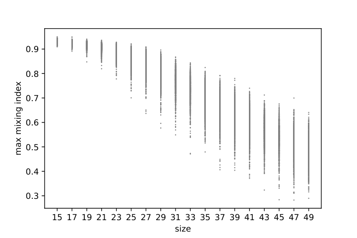
Finally, we compute the 10 percent trimmed mean of the max mixing index, and fit this data to a logistical function in Figure 27.

Figure 27: We compute the 10 percent trimmed mean of the mean mixing index. We fit this data to a logistical function (Eq. (10)) pictured in blue. The parameters are

L=-0.52639764,k=0.52639764,x_{0}=34.83393314

and

b=0.96196691

IV Concluding remarks

In the present paper we have modified the original CELL model plu8 in order to be able to study interactions between multiple CELLs of varying sizes and at different distances. Four different experiments were run. The first of these experiments measured the time it took for two cells to come into contact based on the distance between them. The second of these experiments tested which two cells out of three would merge first. The third of these experiments tested the mobility of cells in relation to cell size. The fourth of these experiments measured the mixing of cytoplasm of two cells in relation to cell size.

Summary of results. Our observed results corroborate multiple expected Physarum behaviors: merging time increases with distance, cells merge with closer cells, cells are more mobile, and smaller cells fuse better. This further validates the CELL model as well as the modified CELL model with multiple CELLs of varying sizes and at varying distances. Furthermore, we have been able to identify the relationship between important characteristics such as speed vs distance (experimental decay) which would have been difficult to determine by experimentally growing Physarum.

From the first experiment, we were able to identify that the correlation between the time to contact and the distance between CELLs is linear. In the second experiment, we determined that CELLs most often merge with the CELLs closest to them and do so quicker than merging with other CELLs. In the third experiment, we determine that there is an exponential decay relationship between measures of mobility (speed, distance from start) and size. In the fourth experiment, we identify the relationship between the mean mixing index and area as exponential decay and the maximum mixing index and size as logistical decay.

Applications. We foresee many applications of our work. In particular, our modified CELL model can be used in the following setups:

(a)

Fusion between multiple CELLs can also be used to model the rise of present day civilization from the early nomadic humans mig1. Each tribe or group is modeled as a cell. Smaller groups or tribes are able to travel faster. As the size grows, they become less and less mobile until permanent settlement occurs. As the groups travel around, they meet other groups where they could merge. As with the results described in this paper, groups closer together have a closer connection than groups further apart.
(b)

Multiple CELLs can be used to model the spread of knowledge among groups of people. Following the ideas of bhansali2020trust, certain groups would begin with certain knowledge, and when they encounter another group, they would combine and both share the knowledge possibly modified. In such way, one could potentially understand the spread and deformation of ideas and information.

In addition, there is more biological work that can be done to verify these results and further validate the CELL model plu8 as well as our generalized CELL model. In particular, each of the experiments done with the CELL model can be done with physical Physarum Polycephalum. In addition, multiple Physarum organisms can share information and communicate prior to protoplasm fusion through the mucus that surrounds Physarum. New models can be developed or existing models can be modified to represent this additional aspect of multiple Physarum fusing.

There is also potential to use multiple Physarum organisms to solve problems a single Physarum has already solved, such as maze solving and tree formation, and this is currently being studied in soon by the authors.

Final comments. Exploring the interaction between multiple Physarum Polycephalum organisms is essential to discovering more about Physarum’s unique ability as a unicellular organism to communicate with other cells and remember past events. More research into Physarum’s unique learning, communication, and memory capabilities will allow us to discover more about the mysteries of human’s and animal’s brains and ability to learn, communicate, and remember.

Acknowledgments. The authors are thankful to MIT PRIMES-USA for the opportunity to conduct this research together, and in particular to Fidel A. Schaposnik for bringing Physarum Polycephalum to our attention after it started growing in his boiler. The work of Laura Schaposnik is partially supported through the NSF grant CAREER DMS 1749013.

Affiliations.
(a) Valley Christian High School, San Jose, USA.
(b) University of Illinois, Chicago, USA.

References

(1) Rinni Bhansali and Laura P Schaposnik. A trust model for spreading gossip in social networks: a multi-type bootstrap percolation model. Proceedings of the Royal Society A, 476(2235):20190826, 2020.
(2) Romain P. Boisseau, David Vogel, and Audrey Dussutour. Habituation in non-neural organisms: evidence from slime moulds. Proceedings of the Royal Society B: Biological Sciences, 283(1829):20160446, 2016.
(3) Atsushi Tero et al. Physarum solver: a biologically inspired method of road-network navigation. Physica A: Statistical Mechanics and its Applications, vol. 363, 2006.
(4) Yukio Gunji, Yukio-Pegio Gunji, Tomohiro Shirakawa, Takayuki Niizato, and Taichi Haruna. Minimal model of a cell connecting amoebic motion andadaptive transport networks. Journal of Theoretical Biology, pages 659–667, 2008.
(5) Maarten Houbraken, Sofie Demeyer, Dimitri Staessens, Pieter Audenaert, Didier Colle, and Mario Pickavet. Fault tolerant network design inspired by physarum polycephalum. Natural Computing, 12(2):277–289, 2013.
(6) Sheryl Hsu and Laura P. Schaposnik. A comparison of multiple physarum organisms in generating spanning trees. In progress.
(7) Jeff Jones. Approximating the behaviours of physarum polycephalum for the construction and minimisation of synthetic transport networks. Unconventional Computation, pages 191–208, 2009.
(8) V.S. Kalogeiton, D.P. Papadopoulos, I.P. Georgilas, G.Ch. Sirakoulis, and A.I. Adamatzky. Cellular automaton model of crowd evacuation inspired by slime mould. International Journal of General Systems, 44(3):354–391, 2015.
(9) P. M. C. Lacey. Developments in the theory of particle mixing. Journal of Applied Chemistry, 4(5):257–268, 1954.
(10) Liang Liu, Yuning Song, Haiyang Zhang, Huadong Ma, and Athanasios V. Vasilakos. Physarum optimization: A biology-inspired algorithm for the steiner tree problem in networks. IEEE Transactions on Computers, 64(3):818–831, 2015.
(11) William H. McNeill. Human migration in historical perspective. Population and Development Review, 10(1):1–18, 1984.
(12) Toshiyuki Nakagaki, Hiroyasu Yamada, and Ágota Tóth. Maze-solving by an amoeboid organism. Nature, 407(6803):470–470, 2000.
(13) Tao Qian, Zili Zhang, Chao Gao, Yuheng Wu, and Yuxin Liu. An ant colony system based on the physarum network. In Ying Tan, Yuhui Shi, and Hongwei Mo, editors, Advances in Swarm Intelligence, pages 297–305, Berlin, Heidelberg, 2013. Springer Berlin Heidelberg.
(14) J. Siriwardana and S. Halgamuge. Fast shortest path optimization inspired by shuttle streaming of physarum polycephalum. 2012 IEEE Congress on Evolutionary Computation, pages 1–8, 2012.
(15) Yahui Sun. Physarum-inspired network optimization: A review. 2019.
(16) Atsushi Tero, Seiji Takagi, Tetsu Saigusa, Kentaro Ito, Dan P. Bebber, Mark D. Fricker, Kenji Yumiki, Ryo Kobayashi, and Toshiyuki Nakagaki. Rules for biologically inspired adaptive network design. Science, 327(5964):439–442, 2010.
(17) Atsushi Tero, Seiji Takagi, Tetsu Saigusa, Kentaro Ito, Daniel Bebber, Mark Fricker, Kenji Yumiki, Ryo Kobayashi, and Toshiyuki Nakagaki. Rules for biologically inspired adaptive network design. Science (New York, N.Y.), 327:439–42, 01 2010.
(18) Shin Watanabe and Atsuko Takamatsu. Transportation network with fluctuating input/output designed by the bio-inspired physarum algorithm. PLOS ONE, 9(2):1–11, 02 2014.
(19) Liu Y, Deng Y, Jusup M, and Wang Z. A biologically inspired immunization strategy for network epidemiology. Journal of theoretical biology, 400:92–102, 2016.
(20) Xiaoge Zhang, Felix T.S. Chan, Andrew Adamatzky, Sankaran Mahadevan, Hai Yang, Zili Zhang, and Yong Deng. An intelligent physarum solver for supply chain network design under profit maximization and oligopolistic competition. International Journal of Production Research, 55(1):244–263, 2017.