Explicit Interaction Network for
Aspect Sentiment Triplet Extraction

Sentiment Analysis is widely used in actual scenarios [27, 28]. There are many variants of sentiment analysis. In terms of task granularity, it can be divided into document level sentiment analysis [29, 30, 31] and aspect level sentiment analysis [32, 17, 33]. Among all variant of sentiment analysis, the most closely related to the ASTE problem is the Aspect-based sentiment analysis (ABSA). ABSA proposed by [34] refers to addressing various sentiment analysis tasks based on specific target words. The most widely known form of ABSA is aspect sentiment classification [35, 36], which aims to predict the sentiment polarity of a given aspect. The model used for the ABSA task usually enhances the interaction between the aspect and the context as much as possible [37, 25], so that the model can pay attention to fine-grained sentiment changes and improve the performance. While Aspect term extract (ATE) [38, 39, 40] requires a model to detect targets from a sentence. ATE is usually treated as sequence labeling problem and solved by CRF-based approaches. Aspect-sentiment pair extraction(ASPE) aims to detect targets and to classifies the sentiment of them [41, 20]. On the top of ATE and ASPE, ASTE extracts the discussed targets, the sentiment of targets, and the opinions explaining why the targets have such sentiment polarities. Compared with ASPE, ASTE can give reasons for sentiment classification, so it is more interpretable. In parallel with our work, [15] inserts four special tags into sentence to guide the encoder to extract compositional feature. [13] uses the machine reading comprehension framework, and propose a query such as ‘whats the sentiment polarity of [price] and [low]’ to classify the sentiment. Both of them try to utilize pairwise compositional features in the sentiment prediction with the specialized templates (input sequences or questions), which are fundamentally different from the proposed table encoder with explicit interaction.

Joint Entity and Relation Extraction (JERE) aims to extract triplets, consisting of named entities and their relations from the sentence, which is similar to ASTE in the form. Many methods have been proposed to solve JERE, such as pipeline extraction methods [42], joint extraction methods [9, 10, 7] and generative methods [43, 44, 45]. Our method is similar to [7] in JERE, which also extracts triplets from sentence through sequence and table encoders. However, our method is different from [7] from both motivation and model designing perspectives: 1) The core contribution of this paper is on the model architecture side of ASTE. We summarize the model architectures of previous work and figure out their potential weakness on defective subtask combination and lack of interaction among subtasks. We thus prove that proper subtask combination and bidirectional interaction among subtasks are the key to successfully from ASTE, which provides actionable insights to NLP community and is different from cfrom the motivation perspective. 2) From model designing perspective, although the model structure is largely inspired by [7], we first point out the importance of the token-pair level feature for ASTE, thus we utilize a table encoder with Multi-Dimension Gated Recurrent Unit (MDGRU) [7, 11, 12] to model it. Note that We do NOT take the credit of designing table encoder. Other encoders, e.g., Transformer [26] (each input corresponds to a token-pair), can also serve the token-pair level feature extractor. In addition, our table encoder also adopt different table filling method, i.e. we use symmetric matrix for table filling while the table in [7] is asymmetric (relation type is directional). At last, the sequence encoder we use is a basic GRU while [7] used a dedicated Transformer variant as basic building block.

Formally, in ASTE, given an input sentence $\boldsymbol{w}=[w_{i}]_{1\leq i\leq N}$, where each $w_{i}$ represents a token in the sentence. We need to extract all triplets $\{(t_{k},s_{k},o_{k})\}_{k=1}^{K}$, where $t_{k}=w_{a:b}$ is a target, $s_{k}\in\{{\rm POS},{\rm NEG},{\rm NEU}\}$ is the sentiment of $t_{k}$, and $o_{k}=w_{c:d}$ is an opinion explaining $s_{k}$, $w_{m:n}$ denotes a span in $\boldsymbol{w}$ with indices from $m$ to $n$.

We split ASTE into target-opinion detection and sentiment classification. In the target-opinion detection, we need to extract all potential targets $\{t_{i}\}_{i=1}^{T}$ and opinions $\{o_{j}\}_{j=1}^{O}$ from the sentence. We solve this subtask via sequence labeling, where the golden tags are the standard BIO scheme.¹¹ 1 {O, B-Target, B-Opinion, I-Target, I-Opinion}.

In the sentiment classification, we need to decide the sentiment of token pairs. We regard this subtask as a table filling problem [9, 10, 7, 4]. Specially, for a sentence including $N$ tokens, we create a sentiment table $T^{s}$ with the shape $N\times N$. An example of table filling is shown in the top-right part of Figure 4(a). Formally, for a sentence with triplets $\{(t_{k},s_{k},o_{k})\}_{k=1}^{K}$, the table cell $(m,n)$ has label $T^{s}_{m,n}=s_{k}$ if $m,n\in C_{t_{k},o_{k}}$,

where $t_{k}=w_{a:b}$, $o_{k}=w_{c:d}$, otherwise, $T^{s}_{m,n}=$ N/A, which indicates that token $i$ and token $j$ have no sentiment relationship. There are four kinds of labels for table cells, {N/A, POS, NEG, NEU}.

We propose a model that jointly performs target-opinion detection and sentiment classification. As shown in Figure 4(a), we use a shared base encoder to extract shared features for two subtasks, and a multi-layer sequence encoder for target and opinion detection. Meanwhile, a multi-layer 2D table encoder is utilized to predict the sentiment of token pairs. We also adopt a bidirectional explicit interaction between two encoders.

To build the implicit interaction between two encoders, given a sentence $\boldsymbol{w}=[w_{i}]_{1\leq i\leq N}$, we first encode each token $w_{i}$ to $\mathbf{x_{i}}\in\mathbb{R}^{d_{w}}$ by an embedding layer, e.g. GloVe or BERT, where ${d_{w}}$ is the embedding dimension. Then we get the shared representation for the subsequent two subtasks,

where $\mathbf{W_{b}}\in\mathbb{R}^{d_{w}\times d_{h}}$ and $\mathbf{b_{b}}\in\mathbb{R}^{d_{h}}$ are trainable parameters.

Since two subtasks are highly interdependent, some features in the table encoder can promote the target-opinion detection. We provide the sequence encoder with the features from the table encoder. Specially, we use a multi-layer table guided sequence encoder. As shown in the left part of Figure 4(b), at layer ($l$), the sequence encoder first encodes the features from the previous layer or the base encoder through GRU,

where $\mathbf{S}^{(l-1)}$ is the output of the previous sequence encoder layer. Then, since each cell of the table encoder corresponds a token pair, motivated by [7], we use Table Guide Attention (TGA) (the green arrow in Figure 4(b)) to aggregate $\bar{\mathbf{S}}^{(l)}$ as follows,

where $i$ denotes the $i$-th head in TGA, $h$ is the number of heads, $\mathbf{T}^{(l)}\in\mathbb{R}^{N\times N\times d_{h}}$ is the hidden state of the table encoder at layer ($l$). The $\mathbf{W_{o}}\in\mathbb{R}^{d_{h}\times d_{h}}$, $\mathbf{v_{i}}\in\mathbb{R}^{d_{h}}$ and $\mathbf{W_{i}}\in\mathbb{R}^{d_{h}\times\frac{d_{h}}{h}}$ are trainable parameters, and we omit their superscripts ($l$) for clarity.

Because the table encoder predicts the token pairs’ sentiment that is generated from the sentiment of target-opinion pairs, some features used to predict targets and opinions can also be used in the table encoder. We thus utilize Sequence Feature Injection (SFI) to bring some helpful features in the sequence encoding process into the table encoder.

As shown in the orange arrow of Figure 4(b), we provide each table cell $(m,n)$ with the feature from corresponding token pair in the sequence encoder as follows,

where $\mathbf{W_{s}}^{(l)}\in\mathbb{R}^{2d_{h}\times d_{h}}$, $\mathbf{b_{s}}^{(l)}\in\mathbb{R}^{d_{h}}$ are trainable parameters, and $\mathbf{X}_{m,n}^{(l)}$ is the input of Equation 11 and Equation 12.

For an input sentence $\boldsymbol{w}=[w_{i}]_{1\leq i\leq N}$, in the target-opinion detection, we utilize the output of the $L$-th layer sequence encoder to predict BIO tags,

where $\mathbf{W_{1}}\in\mathbb{R}^{d_{h}\times 5}$ and $\mathbf{b_{1}}\in\mathbb{R}^{5}$ are trainable parameters, and we use cross-entropy as the loss function,

where $y_{i}^{*}$ is the golden BIO tag of token $x_{i}$. Meanwhile, the sentiment of token pairs is determined by the output of the $L$-th layer table encoder,

where $\mathbf{W_{2}}\in\mathbb{R}^{d_{h}\times 4}$ and $\mathbf{b_{2}}\in\mathbb{R}^{4}$, and the loss function of this subtask is also cross-entropy,

where $y_{m,n}^{*}$ is the golden sentiment of the cell $(m,n)$. The final loss is $\mathcal{L}=\mathcal{L}_{seq}+\mathcal{L}_{table}$. For inference, we get the BIO tag of $x_{i}$ by taking,

and detect targets and opinions according to BIO tags of tokens. For each possible target-opinion pair $(t_{k},o_{k})$, where $t_{k}=w_{a:b}$ and $o_{k}=w_{c:d}$, we predict the sentiment $s_{k}$ by taking,

where $C_{t_{k},o_{k}}$ is defined by Equation 1.

we evaluate our method on ASTE-DATA-V1²² 2 https://github.com/xuuuluuu/SemEval-Triplet-data/tree/master/ASTE-Data-V1-AAAI2020 and ASTE-DATA-V2³³ 3 https://github.com/xuuuluuu/SemEval-Triplet-data/tree/master/ASTE-Data-V2-EMNLP2020. ASTE-DATA-V2 refines its previous version ASTE-DATA-V1 by annotating missing triplets. Both of V1 and V2 have four datasets, 14Rest, 15Rest, 16Rest in restaurant domain, and 14Lap in laptop domain. The details about four datasets of ASTE-DATA-V1 and ASTE-DATA-V2 are included in Table I and Table II, respectively. Moreover, following previous work, e.g., [2, 3, 4], we adopt the precision (P.), recall (R.) and micro F1-measure (F1.) as our evaluation metrics for triplet extraction.

For systematic comparisons, we introduce a variety of baselines,

• •

  CMLA+ [2] is modified from CMLA [18]. CMLA use attention mechanism to capture the relationship between words, and extract targets with sentiment together. CMLA+ add an MLP on CMLA to determine whether a triplet is correct in the matching stage.

• •

  RINANTE+ [2] is modified from RINANTE [19], which uses LSTM-CRF and fuses rules as weak supervision to capture dependency relations of words. The way RINANTE+ determine the correctness of a triplet is the same as CMLA+.

• •

  Li-unified-R [2] is modified from [20], which extracts targets, sentiment and opinion spans respectively based on a multi-layer LSTM neural architecture. The way Li-unified-R determine the correctness of a triplet is the same as CMLA+.

• •

  Peng20 [2] also decomposes triplet extraction to two stages: extracts unified target-sentiment and opinions via GCN first, then pairs the two results from the results before.

• •

  JET [3] regards ASTE as a sequence labeling problem based on unified tags. JET has two variants: ${\rm JET}_{t}$ predict the target, the sentiment of target and the corresponding opinion. ${\rm JET}_{o}$ predict the opinion, the sentiment of the opinion and the corresponding target.

• •

  OTE [4] utilizes a multi-task framework to solve ASTE, which learns joint features of different subtasks via a shared encoder, then predicts targets, opinions by sequence labeling and use a biaffine layer to predict sentiment.

• •

  GTS [5] formulates ASTE as an unified grid tagging task. It first extracts sentiment feature of each token, and then get the initial prediction probabilities of toke pairs based on these token-level features. At last, it designs a gird inference strategy to modeling the mutual interactions of all probabilities, and performs the final prediction.

• •

  ${\rm\mathbf{S^{3}E^{2}}}$ [16] exploits the syntactic and semantic relationships between the triplet elements with a semantic and syntactic enhanced module.

• •

  [13] formulates ASTE as a machine reading comprehension problem, and proposes three types of queries to extract targets, opinions and the sentiment polarities of target-opinion pairs, respectively.

• •

  Dual-MRC [21] constructs two machine reading comprehension problems to slove ASTE and other Aspect based sentiment analysis tasks with joint training two BERT-MRC models.

• •

  [15] proposes a two-stage model, which first extracts targets and opinions, and then inserts special tags into sentence to identify the specific target-opinion pair and finally predict the sentiment polarity of this pair.

• •

  [14] formulates ASTE as a sequence-to-sequence generation problem, and utilizes pre-trained sequence-to-sequence model BART [22] with teacher forcing training to generate targets, opinions and sentiment polarities directly.

For embedding layer, following [3], we use GloVe with dimension $300$ or BERT-base-uncased⁴⁴ 4 https://huggingface.co/bert-base-uncased/tree/main without fine-tuning. For the sequence encoder, the hidden size $d_{h}$, the number of head $h$ and layer $L$ are set to $200$, $8$ and $3$, respectively. For the table encoder, the dimension of cell vector, the hidden size of MDGRU and the layer number $L$ are set to $200$, $200$ and $3$, respectively. We use Adam [23] as our optimizer with inverse time learning rate decay, the decay rate is $0.05$ and decay step is $1000$, and the learning rate is set to $0.001$. Dropout [24] is set to $0.5$, and the batch size is $6$. We select the model parameter with the best F1 on the valid dataset and apply it to the test data for evaluation. Details of all the hyper-parameters are provided in Table V.

Table III reports the results of our model and baseline models. Firstly, when using GloVe, our model achieves the best results on all eight datasets. Secondly, when using contextual pre-trained model, our BERT-based model outperforms all previous BERT-based methods. Compared with [14], which uses BART pre-trained model, on the one hand, our BERT-based model achieves better results on six datasets, e.g., $5.88$F1 points improvement on V2-14Rest, and only achieves slight lower results on two datasets, i.e., $0.54$F1 points on V1-14Rest and $0.47$F1 points on V1-16Rest. On the other hand, the pre-trained parameters of BART-base model used in [14] is $29$M more than BERT-base parameters used in our model (nearly $30$% parameters of BERT-base). Thirdly, our GloVe-based model even beats previous popular BERT-based models, e.g., JET, OTE. In conclusion, we provides a new state-of-the-art solution for ASTE, since we carefully design the combination of subtasks, introduce a table encoder to extract compositional features of target-opinion pairs and strengthen the explicit interaction between subtasks.

In ASTE, the interaction among different subtasks is important for three elements in the triplet are closely related. On top of implicit interaction, we introduce a bidirectional explicit interaction between two subtasks with table guide attention (TGA) and sequence feature injection (SFI). In this part, we explore the effect of TGA and SFI.

Firstly, we remove the TGA and SFI from the model in turn. Specifically, when removing TGA, we follow [25] and utilize the multi-head self-attention [26] to aggregate features in the sequence encoder. When removing SFI, we calculate the input for two MDGRUs with the output of the base encoder. As shown in Table IV, bidirectional explicit interaction model (Both) outperforms unidirectional explicit interaction models (w/o SFI and w/o TGA), in addition, w/o SFI and w/o TGA beat the model without explicit interaction (w/o Both). Secondly, we share the parameters of two encoders in different layers. When the number of layers in the model increases, as shown in Figure 6, the performance of the model without explicit interaction does not improve, however, the model with explicit interactions can benefit from the increasing layer number. Since the number of parameters remains unchanged when sharing parameters, we conclude that the model performance benefits from the explicit interactions. These results show the importance of the explicit interaction in ASTE.

The table encoder explicitly injects the inductive bias of compositional token pair representation into model, so it can reduce the erroneous predictions on non-existent triplets. In this part, we explore the effect of the table encoder. Our table encoder, biaffine scorer [8] of OTE and GTS establish the similar tabular like structures. However, our table encoder extracts token-pair level features and the other two methods only model token level features. To better explore our table encoder’s advantage, we only use the sequence encoder (OnlySeq) and the table encoder (OnlyTab) to solve ASTE separately. For OnlySeq, following OTE, we utilize biaffine scorer to establish the table for sentiment classification. For OnlyTab, we use the diagonal cells to detect targets and opinions.⁵⁵ 5 We set the number of layers of OnlyTab and OnlySeq to $3$ and $6$, respectively, so these two models have about the same number of parameters.

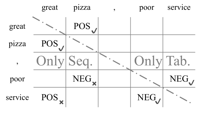
As shown in Table VI, OnlyTab outperforms OnlySeq (all 4 datasets) and GTS (3 out of 4 datasets), which shows the importance of compositional feature for ASTE. The performance of OnlyTab on 15Rest is slightly lower than that of GTS, we think the reason is that there are relatively small number of multiple triplets on 15Rest as shown in Table VII. In addition, we also conduct a case study to intuitively show the effect of our table encoder, as shown in Figure 7, the top-right and bottom-left triangles of the matrix represent the sentiment classification results of OnlyTab and OnlySeq, respectively. In this case, the sentence contains two opinions, great and poor, which express positive and negative sentiment. Since the sequence encoder extracts features at the token level, the sentiment of great and poor misleads the classification results, i.e., (service, POS, great) and (pizza, NEG, poor). However, the table encoder, which extracts sentiment features at the token-pair level, obtains the right results. These results show that modeling the compositional feature of target-opinion pair is important for ASTE, and the table encoder plays a vital role for this propose.

ASTE is a composite triplet extraction task, which consists of 3 atom subtasks, and a reasonable subtask combination is essential for ASTE. Although solving all of 3 atom subtasks by a single module, e.g., GTS, ${\rm JET_{o}}$ and ${\rm JET_{t}}$ can enhance the interaction of different subtasks, they also effect each others. As shown in Table VI. Our full model Both outperforms OnlyTab, which extracts targets, opinions and sentiment through a single module like GTS. We think enhancing the interaction of subtasks by explicit interaction mechanisms is better than formulate different subtasks as a unified task. Through explicit interaction, each module can utilize the useful information and drop the harmful information from other subtasks. However, when solving all subtasks through a single module, the single module must pay attention to all subtasks, so for a subtask, some harmful information from other subtasks can not be dropped optionally. Such a phenomenon of mutual interference is also found in other tasks [7, 42].

Our model achieves noticeable performance gain over previous methods. In this part, we explore the advantage of our model. Firstly, compared with previous method JET, which has ill task formulation and extracts token-level feature, we find out that our model has advantage in dealing sentences with multiple triplets. As shown in Table VII, the situation that one sentence has multiple triplets is usual, e.g., such cases reach a ratio from $34.67\%$ on 15Rest to $58.21\%$ on 14Rest, and our model achieves more considerable performance gain on datasets with larger ratio ${\rm R_{t>1}}$. We further divide the sentences according to the number of triplets in them. As shown in Figure 8, as the number of triplets in a sentence increases, our model outperforms other models more obviously. These results show that our model has more advantages over other methods in handling such a changeling but common situation. We also conduct a case study to show this intuitively. The sentence in Figure 9 has $5$ potential opinions (colored by green), $5$ targets (colored by blue) and $5$ golden triplets. Our model correctly extracts all triplets. however, ${\rm JET_{o}}$ misses two golden triplets of opinion delectable for its unreasonable subtask combination, and both ${\rm JET_{o}}$ and GTS extract two false triplets due to they are influenced by the potential opinion words with strong sentiment, e.g., pleasantly and uncrowded. We guess the performance gain in such a challenging situation benefits from our subtask combination, the explicit interaction mechanisms and the table encoder. Firstly, our subtask combination is more in line with human cognition, i.e., judging sentiment based on both target and opinion. Secondly, more triplets in one sentence cause the extraction more difficult, while our explicit interaction mechanisms can make different subtasks better promote each other, which helps the model perform stably, At last, since every target and every opinion may contain sentiment and form a triplet, more targets and opinions in one sentence will exacerbate the erroneous predictions on non-existent triplets, while our table encoder can alleviate this by extracting features at the token-pair level.

References

- [1] R. K. Bakshi, N. Kaur, R. Kaur, and G. Kaur, “Opinion mining and sentiment analysis,” in 2016 3rd international conference on computing for sustainable global development (INDIACom). IEEE, 2016, pp. 452–455.
- [2] H. Peng, L. Xu, L. Bing, F. Huang, W. Lu, and L. Si, “Knowing what, how and why: A near complete solution for aspect-based sentiment analysis.” in AAAI, 2020, pp. 8600–8607.
- [3] L. Xu, H. Li, W. Lu, and L. Bing, “Position-aware tagging for aspect sentiment triplet extraction,” in Proceedings of the 2020 Conference on Empirical Methods in Natural Language Processing (EMNLP), 2020, pp. 2339G–2349.
- [4] C. Zhang, Q. Li, D. Song, and B. Wang, “A multi-task learning framework for opinion triplet extraction,” in Proceedings of the 2020 Conference on Empirical Methods in Natural Language Processing: Findings, 2020, pp. 819–828.
- [5] Z. Wu, C. Ying, F. Zhao, Z. Fan, X. Dai, and R. Xia, “Grid tagging scheme for aspect-oriented fine-grained opinion extraction,” in Findings of the Association for Computational Linguistics: EMNLP 2020. Online: Association for Computational Linguistics, Nov. 2020, pp. 2576–2585. [Online]. Available: https://www.aclweb.org/anthology/2020.findings-emnlp.234
- [6] F. Li, Z. Wang, S. C. Hui, L. Liao, D. Song, J. Xu, G. He, and M. Jia, “Modularized interaction network for named entity recognition,” in Proceedings of the 59th Annual Meeting of the Association for Computational Linguistics and the 11th International Joint Conference on Natural Language Processing (Volume 1: Long Papers), 2021, pp. 200–209.
- [7] J. Wang and W. Lu, “Two are better than one: Joint entity and relation extraction with table-sequence encoders,” in Proceedings of the 2020 Conference on Empirical Methods in Natural Language Processing (EMNLP), 2020, pp. 1706–1721.
- [8] T. Dozat and C. D. Manning, “Deep biaffine attention for neural dependency parsing,” arXiv preprint arXiv:1611.01734, 2016.
- [9] P. Gupta, H. Schütze, and B. Andrassy, “Table filling multi-task recurrent neural network for joint entity and relation extraction,” in Proceedings of COLING 2016, the 26th International Conference on Computational Linguistics: Technical Papers, 2016, pp. 2537–2547.
- [10] M. Zhang, Y. Zhang, and G. Fu, “End-to-end neural relation extraction with global optimization,” in Proceedings of the 2017 Conference on Empirical Methods in Natural Language Processing, 2017, pp. 1730–1740.
- [11] A. Graves, S. Fernández, and J. Schmidhuber, “Multi-dimensional recurrent neural networks,” in International conference on artificial neural networks. Springer, 2007, pp. 549–558.
- [12] K. Cho, B. van Merriënboer, C. Gulcehre, D. Bahdanau, F. Bougares, H. Schwenk, and Y. Bengio, “Learning phrase representations using rnn encoder–decoder for statistical machine translation,” in Proceedings of the 2014 Conference on Empirical Methods in Natural Language Processing (EMNLP), 2014, pp. 1724–1734.
- [13] S. Chen, Y. Wang, J. Liu, and Y. Wang, “Bidirectional machine reading comprehension for aspect sentiment triplet extraction,” arXiv preprint arXiv:2103.07665, 2021.
- [14] H. Yan, J. Dai, X. Qiu, Z. Zhang et al., “A unified generative framework for aspect-based sentiment analysis,” arXiv preprint arXiv:2106.04300, 2021.
- [15] L. Huang, P. Wang, S. Li, T. Liu, X. Zhang, Z. Cheng, D. Yin, and H. Wang, “First target and opinion then polarity: Enhancing target-opinion correlation for aspect sentiment triplet extraction,” arXiv preprint arXiv:2102.08549, 2021.
- [16] Z. Chen, H. Huang, B. Liu, X. Shi, and H. Jin, “Semantic and syntactic enhanced aspect sentiment triplet extraction,” arXiv preprint arXiv:2106.03315, 2021.
- [17] H. Yang, B. Zeng, J. Yang, Y. Song, and R. Xu, “A multi-task learning model for chinese-oriented aspect polarity classification and aspect term extraction,” Neurocomputing, vol. 419, pp. 344–356, 2019.
- [18] W. Wang, S. J. Pan, D. Dahlmeier, and X. Xiao, “Coupled multi-layer attentions for co-extraction of aspect and opinion terms,” in Thirty-First AAAI Conference on Artificial Intelligence, 2017.
- [19] H. Dai and Y. Song, “Neural aspect and opinion term extraction with mined rules as weak supervision,” in Proceedings of the 57th Annual Meeting of the Association for Computational Linguistics, 2019, pp. 5268–5277.
- [20] X. Li, L. Bing, P. Li, and W. Lam, “A unified model for opinion target extraction and target sentiment prediction,” in Proceedings of the AAAI Conference on Artificial Intelligence, vol. 33, 2019, pp. 6714–6721.
- [21] Y. Mao, Y. Shen, C. Yu, and L. Cai, “A joint training dual-mrc framework for aspect based sentiment analysis,” arXiv preprint arXiv:2101.00816, 2021.
- [22] M. Lewis, Y. Liu, N. Goyal, M. Ghazvininejad, A. Mohamed, O. Levy, V. Stoyanov, and L. Zettlemoyer, “BART: Denoising sequence-to-sequence pre-training for natural language generation, translation, and comprehension,” in Proceedings of the 58th Annual Meeting of the Association for Computational Linguistics. Online: Association for Computational Linguistics, Jul. 2020, pp. 7871–7880. [Online]. Available: https://www.aclweb.org/anthology/2020.acl-main.703
- [23] D. P. Kingma and J. Ba, “Adam: A method for stochastic optimization,” arXiv preprint arXiv:1412.6980, 2014.
- [24] N. Srivastava, G. Hinton, A. Krizhevsky, I. Sutskever, and R. Salakhutdinov, “Dropout: a simple way to prevent neural networks from overfitting,” The journal of machine learning research, vol. 15, no. 1, pp. 1929–1958, 2014.
- [25] Y. Song, J. Wang, T. Jiang, Z. Liu, and Y. Rao, “Attentional encoder network for targeted sentiment classification,” arXiv preprint arXiv:1902.09314, 2019.
- [26] A. Vaswani, N. Shazeer, N. Parmar, J. Uszkoreit, L. Jones, A. N. Gomez, Ł. Kaiser, and I. Polosukhin, “Attention is all you need,” in Advances in neural information processing systems, 2017, pp. 5998–6008.
- [27] A. Agarwal, B. Xie, I. Vovsha, O. Rambow, and R. J. Passonneau, “Sentiment analysis of twitter data,” in Proceedings of the workshop on language in social media (LSM 2011), 2011, pp. 30–38.
- [28] X. Fang and J. Zhan, “Sentiment analysis using product review data,” Journal of Big Data, vol. 2, no. 1, p. 5, 2015.
- [29] Q. Le and T. Mikolov, “Distributed representations of sentences and documents,” in International conference on machine learning. PMLR, 2014, pp. 1188–1196.
- [30] Z. Zhao, “Learning document embeddings by predicting n-grams for sentiment classification of long movie reviews,” in Workshop Contribution (ICLR), 2016.
- [31] T. Thongtan and T. Phienthrakul, “Sentiment classification using document embeddings trained with cosine similarity,” in Proceedings of the 57th Annual Meeting of the Association for Computational Linguistics: Student Research Workshop, 2019, pp. 407–414.
- [32] L. Dong, F. Wei, C. Tan, D. Tang, M. Zhou, and K. Xu, “Adaptive recursive neural network for target-dependent twitter sentiment classification,” in Proceedings of the 52nd annual meeting of the association for computational linguistics (volume 2: Short papers), 2014, pp. 49–54.
- [33] A. Rietzler, S. Stabinger, P. Opitz, and S. Engl, “Adapt or get left behind: Domain adaptation through bert language model finetuning for aspect-target sentiment classification,” in Proceedings of The 12th Language Resources and Evaluation Conference, 2020, pp. 4933–4941.
- [34] S. Manandhar, “Semeval-2014 task 4: aspect based sentiment analysis,” in Proceedings of the 8th international workshop on semantic evaluation (SemEval 2014), 2014.
- [35] P. Chen, Z. Sun, L. Bing, and W. Yang, “Recurrent attention network on memory for aspect sentiment analysis,” in Proceedings of the 2017 conference on empirical methods in natural language processing, 2017, pp. 452–461.
- [36] L. Xu, L. Bing, W. Lu, and F. Huang, “Aspect sentiment classification with aspect-specific opinion spans,” arXiv preprint arXiv:2010.02696, 2020.
- [37] D. Ma, S. Li, X. Zhang, and H. Wang, “Interactive attention networks for aspect-level sentiment classification,” arXiv preprint arXiv:1709.00893, 2017.
- [38] B. Yang and C. Cardie, “Extracting opinion expressions with semi-markov conditional random fields,” in Proceedings of the 2012 Joint Conference on Empirical Methods in Natural Language Processing and Computational Natural Language Learning, 2012, pp. 1335–1345.
- [39] X. Li, L. Bing, P. Li, W. Lam, and Z. Yang, “Aspect term extraction with history attention and selective transformation,” in Proceedings of the 27th International Joint Conference on Artificial Intelligence, 2018, pp. 4194–4200.
- [40] D. Ma, S. Li, and H. Wang, “Joint learning for targeted sentiment analysis,” in Proceedings of the 2018 Conference on Empirical Methods in Natural Language Processing, 2018, pp. 4737–4742.
- [41] E. Ekinci and S. İlhan Omurca, “An aspect-sentiment pair extraction approach based on latent dirichlet allocation for turkish,” International Journal of Intelligent Systems and Applications in Engineering, vol. 6, no. 3, pp. 209–213, 2018.
- [42] Z. Zhong and D. Chen, “A frustratingly easy approach for joint entity and relation extraction,” arXiv preprint arXiv:2010.12812, 2020.
- [43] T. Nayak and H. T. Ng, “Effective modeling of encoder-decoder architecture for joint entity and relation extraction,” in Proceedings of the AAAI Conference on Artificial Intelligence, vol. 34, no. 05, 2020, pp. 8528–8535.
- [44] S. Xiao, M. Song et al., “A text-generated method to joint extraction of entities and relations,” Applied Sciences, vol. 9, no. 18, p. 3795, 2019.
- [45] D. Sui, Y. Chen, K. Liu, J. Zhao, X. Zeng, and S. Liu, “Joint entity and relation extraction with set prediction networks,” arXiv preprint arXiv:2011.01675, 2020.