![[Uncaptioned image]](2106.10897v1/TitlePage1.png)
Abstract
In this thesis, we study chiral topological phases of 2+1 dimensional quantum matter. Such phases are abstractly characterized by their non-vanishing chiral central charge , a topological invariant which appears as the coefficient of a gravitational Chern-Simons (gCS) action in bulk, and of corresponding gravitational anomalies at boundaries. The chiral central charge is of particular importance in chiral superfluids and superconductors (CSF/Cs), where particle-number symmetry is broken, and is, in some cases, the only topological invariant characterizing the system. However, as opposed to invariants which can be probed by gauge fields in place of gravity, the concrete physical implications of in the context of condensed matter physics is quite subtle, and has been the subject of ongoing research and controversy. The first two parts of this thesis are devoted to the physical interpretation of the gCS action and gravitational anomalies in the context of CSF/Cs, where they are of particular importance, but have nevertheless remained poorly understood.
As a first approach, we demonstrate that, at low energy, fermionic excitations in -wave CSF/Cs experience an emergent relativistic Riemann-Cartan geometry, described by the superconducting order parameter and background gauge field. This description is then used to infer gCS energy-momentum responses to a space-time dependent order parameter, and relate these to an order parameter induced gravitational anomaly. The presence of torsion in the emergent geometry, as well as the multiplicity of low energy spinors in the case of lattice systems, lead to additional effects which are not of topological origin, but nevertheless mimic closely the above gCS physics. We show how these different phenomena can be disentangled.
We then take on a fully non-relativistic analysis of CSFs, obtaining a low energy effective field theory that consistently captures both their chiral Goldstone mode and their non-relativistic gCS action. Using the theory we find that cannot be extracted from a measurement of the odd viscosity tensor alone, despite naive expectation based on previous work. Nevertheless, a related observable, termed ‘improved odd viscosity’, does allow for the bulk measurement of . Additional results of the same spirit are found in Galilean invariant CSFs.
Finally, we turn to a seemingly unrelated aspect of chiral topological phases - their computational complexity. The infamous sign problem leads to an exponential complexity in Monte Carlo simulations of generic many-body quantum systems. Nevertheless, many phases of matter are known to admit a sign-problem-free representative, allowing an efficient classical simulation. Motivated by long standing open problems in many-body physics, as well as fundamental questions in quantum complexity, the possibility of intrinsic sign problems, where a phase of matter admits no sign-problem-free representative, was recently raised but remains largely unexplored. Here, we establish the existence of an intrinsic sign problem in a broad class of chiral topological phases, defined by the requirement that is not the topological spin of an anyon. Within this class, we exclude the possibility of ‘stoquastic’ Hamiltonians for bosons, and of sign-problem-free determinantal Monte Carlo algorithms for fermions. We obtain analogous results for phases that are spontaneously chiral, and present evidence for an extension of our results that applies to both chiral and non-chiral topological matter.
Acknowledgments
Adding a grain of sand to one of the very many and ever growing summits of the mountain range known as ‘human knowledge’ is truly a great privilege. The climb, however, is usually no easy task, and the one that produced this thesis was no exception. Here, I would like to pause and thank those who supported me en route.
First, I am grateful to my advisor Ady Stern, who suggested an unorthodox but tailor made research direction, and collaborated with me on the first and most challenging part of the work. Ady is a formidable physicist as well as a generous advisor, and provided a rare combination of support and freedom in my research. It was also wonderful to work under someone who views laughter as a way of life.
Subsequent work was performed in mostly long distance but close collaborations with Sergej Moroz, Carlos Hoyos, Félix Rose, Zohar Ringel and Adam Smith. In particular, Sergej, Carlos and Zohar served as additional mentors, each with his own unique style of doing research. I also benefited greatly from extensive discussions with Paul Wiegmann, Andrey Gromov, Ryan Thorngren, Weihan Hsiao, Semyon Klevtsov, Barry Bradlyn and Thomas Kvorning.
The members of my PhD advisory committee, Micha Berkooz and David Mross, as well as my senior group members, Yuval Baum, Ion Cosma Fulga, Jinhong Park, Raquel Queiroz and Tobias Holder, provided much needed physical and meta-physical advice along the way. Our administrative staff, Hava Shapira, Merav Laniado, Einav Yaish, Inna Dombrovsky, Yuval Toledo and Yuri Magidov, sustained an incredibly efficient and warm work environment. I also thank my fellow graduate students Eyal Leviatan, Ori Katz, Dan Klein, Avraham Moriel, Shaked Rozen, Asaf Miron, Yotam Shpira, Adar Sharon, Dan Dviri and, of course, Yuval Rosenberg, who dragged me to the Weizmann institute when we were kids, and got me hooked on physics.
Zooming out, I am grateful to my parents Sharona and Gabi, for their continued support in whatever I choose to do, and to my wife and best friend Adi, for making my life happy and balanced. Since we became parents, my work would not have been possible without Adi’s backing, in particular since the spreading of Coronavirus, which eliminated some of our support systems, as well as the distinction between work and home. Finally, I thank our boys Adam and Shlomi for their smiles, laughter, and curiosity - a reminder of why I was drawn to science in the first place.
Publications
This thesis is based on the following publications:
- •
Reference [1]: Omri Golan and Ady Stern. Probing topological superconductors with emergent gravity. Phys. Rev. B, 98:064503, 2018.
- •
Reference [2]: Omri Golan, Carlos Hoyos, and Sergej Moroz. Boundary central charge from bulk odd viscosity: Chiral superfluids. Phys. Rev. B, 100:104512, 2019.
- •
Reference [3]: Omri Golan, Adam Smith, and Zohar Ringel. Intrinsic sign problem in fermionic and bosonic chiral topological matter. Phys. Rev. Research, 2:043032, 2020.
Complementary results are obtained in:
- •
Reference [4]: Félix Rose, Omri Golan, and Sergej Moroz. Hall viscosity and conductivity of two-dimensional chiral superconductors. SciPost Phys., 9:6, 2020.
- •
Reference [5]: Adam Smith, Omri Golan, and Zohar Ringel. Intrinsic sign problems in topological quantum field theories. Phys. Rev. Research, 2:033515, 2020.
1 Introduction and summary
1.1 Overview
The study of topological phases of matter began in 1980, when the Hall conductivity in a two-dimensional electron gas was measured to be an integer multiple of , to within a relative error of [6], subsequently reduced below [7]. Following this discovery, it was theoretically understood that in many-body quantum systems, certain physical observables must be precisely quantized, under the right circumstances [8, 9]. Around the same time, quantum field theorists extensively studied the phenomena of anomalies [10, 11, 12], where classical symmetries and conservation laws are quantum mechanically violated, and discovered the seemingly exotic anomaly inflow mechanism [13, 14], which physically interprets anomalies in terms of topological effective actions in higher space-time dimensions. It was only later understood that topological effective actions and anomalies actually capture the essential physics of topological phases of matter, and even classify them [15, 16, 17, 18, 19, 20].
In particular, 2+1D gapped chiral topological phases are characterized by a gravitational Chern-Simons (gCS) action [21, 22, 23, 24, 25] and corresponding 1+1D gravitational anomalies [10, 12, 26], having the chiral central charge as a precisely quantized coefficient, or topological invariant. The chiral central charge is of particular importance in chiral superfluids and superconductors [15, 27], where particle-number symmetry is broken spontaneously or explicitly, and is, in some cases, the only topological invariant characterizing the system at low energy. However, as opposed to topological invariants related to gauge fields for internal symmetries in place of gravity, the concrete physical implications of (and even its very definition) in the context of condensed matter physics is quite subtle, and has been the subject of ongoing research and controversy [28, 15, 29, 30, 31, 32, 17, 33, 34, 35, 36, 37, 38, 39, 40, 41, 42, 43, 44, 45, 46, 47, 48, 49, 50, 51, 52, 53, 54, 55]. The first goal of this thesis is to physically interpret the chiral central charge in the context of chiral superfluids and superconductors, where it is of particular importance, but has nevertheless remained poorly understood. This goal is pursued in Sec.2-3.
A seemingly unrelated aspect of chiral topological phases is the complexity of simulating them on classical (as opposed to quantum) computers. It is generally believed that chiral topological matter is ’hard’ to simulate efficiently with classical resources. Concretely, it is known that chiral topological phases do not admit local commuting projector Hamiltonians [56, 57, 58, 59, 54], nor do they admit local Hamiltonians with a PEPS state as an exact ground state [60, 61, 62, 63]. We will be interested in quantum Monte Carlo (QMC) simulations, arguably the most important tools in computational many-body quantum physics [64, 65, 66, 67, 68, 69, 70, 71], and in the infamous sign problem, which is the generic obstruction to an efficient QMC simulation [72, 73, 74].
The accumulated experience of QMC practitioners suggests that the sign problem was never solved in chiral topological matter. Since these phases are abstractly defined by their non-vanishing chiral central charge, one may suspect that the chiral central charge and related gravitational phenomena pose an obstruction to sign-problem-free QMC. Such an obstruction is termed intrinsic sign problem [75, 76], and is of interest beyond the context of chiral topological matter, as it is widely accepted that long-standing open problems in many-body quantum physics, such as the nature of high-temperature superconductivity [77, 78, 79, 80], dense nuclear matter [81, 82, 83], and the fractional quantum Hall state at filling [84, 85, 86, 87, 88, 55], remain open because no solution to the sign problem in a relevant model has thus far been found. Since the aforementioned open problems are all fermionic, we are particularly motivated to study the possibility of intrinsic sign problems in fermionic matter. The second goal of this thesis, pursued in Sec.4, is to establish the existence of an intrinsic sign problem in chiral topological phases of matter, based on their non-vanishing chiral central charge, and with an emphasis on fermionic systems.
1.2 Chiral topological matter
A gapped local many-body quantum Hamiltonian is said to be in a topological phase of matter if it cannot be deformed to a trivial reference Hamiltonian, without closing the energy gap or violating locality. If a symmetry is enforced, only symmetric deformations are considered, and it is additionally required that the symmetry is not spontaneously broken [89, 90]. For Hamiltonians defined on a lattice, a natural trivial Hamiltonian is given by the atomic limit of decoupled lattice sites, where the symmetry acts independently on each site. In this thesis we consider both lattice and continuum models.
Topological phases with a unique ground state on the 2-dimensional torus exist only with a prescribed symmetry group11 1 A subtle point is that the minimal symmetry group for fermionic systems is fermion parity - the group generated by , where is the fermion number. This should be contrasted with bosonic systems, which may have no symmetries. and are termed symmetry protected topological phases (SPTs) [91, 92, 93]. When such phases are placed on the cylinder, they support anomalous boundary degrees of freedom which cannot be realized on isolated 1-dimensional spatial manifolds, as well as corresponding quantized bulk response coefficients. Notable examples are the integer quantum Hall states, topological insulators, and topological superconductors [94]. Topological superconductivity and superfluidity will be discussed in detail in Sec.1.4.
Topological phases with a degenerate ground state subspace on the torus are termed topologically ordered, or symmetry enriched if a symmetry is enforced [95, 96]. Beyond the phenomena exhibited by SPTs, these support localized quasiparticle excitations with anyonic statistics and fractional charge under the symmetry group. Notable examples are fractional quantum Hall states [97, 98], quantum spin liquids [99], and fractional topological insulators [100, 101].
In this thesis, we consider chiral topological phases, where the boundary degrees of freedom that appear on the cylinder propagate unidirectionally. At energies small compared with the bulk gap, the boundary can be described by a chiral conformal field theory (CFT) [102, 103], while the bulk reduces to a chiral topological field theory (TFT) [104, 19], see Fig.1(a). Such phases may be bosonic and fermionic, and may be protected or enriched by an on-site symmetry, but we will not make use of this symmetry in our analysis - only the chirality of the phase will be used.
A notable example for chiral topological phases is given by Chern insulators [105, 106, 107]: SPTs protected by the fermion number symmetry, which admit free-fermion Hamiltonians. The single particle spectrum of a Chern insulator on the cylinder is depicted in Fig.1(b). Another notable example are the topologically ordered Kitaev spin liquids [104, 108], which can be described by Majorana fermions with a single particle spectrum similar to Fig.1(b), coupled to a (fermion-parity) gauge field. Note that the velocity of the boundary CFT is a non-universal parameter which generically changes as the microscopic Hamiltonian is deformed. More generally, different chiral branches may have different velocities.

The chirality of the boundary CFT and bulk TFT is manifested by their non-vanishing chiral central charge , which is rational and universal - it is a topological invariant with respect to continuous deformations of the Hamiltonian which preserve locality and the bulk energy gap, and therefore constant throughout a topological phase [109, 104, 39, 42]. On the boundary is defined with respect to an orientation of the cylinder, so the two boundary components have opposite chiral central charges. Since, as described below, is much better understood from the boundary perspective, we sometimes refer to it as the boundary chiral central charge. A main theme of this thesis is the study of from the bulk perspective, and the relation between the two perspectives implied by the anomaly inflow mechanism.
1.3 Geometric physics in chiral topological matter
The non-vanishing of implies a number of geometric, or ’gravitational’, physical phenomena [102, 103, 34, 43, 42, 44]. In particular, the boundary supports a non-vanishing energy current , which receives a correction
| (1.1) |
at a temperature , and in the thermodynamic limit , where is the circumference of the cylinder. Note that we set and throughout. Within CFT, this correction is universal since it is independent of . Taking the two counter propagating boundary components of the cylinder into account, and placing these at slightly different temperatures, leads to a thermal Hall conductance [110, 15, 111], a prediction that recently led to the first measurements of [112, 113, 84, 114].
In analogy with Eq.(1.1), the boundary of a chiral topological phase also supports a non-vanishing ground state (or ) momentum density , which receives a universal correction on a cylinder with finite circumference . The details of this finite-size correction will be described in Sec.4, where it is used to relate the chiral central charge (as well as the topological spins of anyon excitations) to the complexity of simulating chiral topological matter on classical computers.
Abstractly, both and corrections described above follow directly from the (chiral) Virasoro anomaly, or Virasoro central extension, which defines in 2D CFT. Equivalently, these corrections can be understood in terms of the ’global’ gravitational anomaly - the complex phase accumulated by a CFT partition function on the torus under a Dehn twist [102, 103]. This anomaly is termed ’global’ since the Dehn twist is a large coordinate transformation, or more accurately, an element of the diffeomorphism group of the torus, which lies outside of the connected component of the identity. The Dehn twist is therefore the geometric analog of the large gauge transformation used in the celebrated Laughlin argument, and an attempt has been made to follow this analogy and produce a ’thermal Laughlin argument’ [50].
The chiral central charge also implies a ’local’, or ’perturbative’ gravitational anomaly, which, at least in the context of relativistic QFT in curved space-time, physically corresponds to the non-conservation of energy-momentum in the presence of curvature gradients [10, 12, 26]. Through the anomaly inflow mechanism, or in more physical terms, through bulk+boundary energy-momentum conservation, this boundary anomaly implies a gravitational Chern-Simons (gCS) term in the effective action describing the 2+1D bulk of a chiral topological phase [21, 22, 23, 24, 25]22 2 Whether the gCS term matches the boundary global gravitational anomaly as well is, to the best of my knowledge, an open problem.. In turn, the gCS term implies a quantized energy-momentum-stress response to curvature gradients, in the bulk 33 3 In fact, the gCS contribution to the energy-momentum-stress tensor is proportional to the mathematically important Cotton tensor of the metric [115]. .
Though the gCS term is relatively well understood in the context of relativistic QFT, its concrete physical content in the non-relativistic setting of condensed matter physics is quite subtle, due to the following reasons:
- 1.
Physically, the actual gravitational field of the earth is usually negligible in condensed matter experiments. It is therefore clear that the adjective ’gravitational’ used above cannot be taken literally, and requires further interpretation. Namely, one must find a physical probe relevant in condensed matter experiments, which will somehow mimic the effects of a strong gravitational field. This scenario is often referred to as ’analog gravity’ or ’emergent gravity’ [27]. Mathematically, this corresponds to a physically accessible geometric structure on the space-time occupied by the system of interest, in the spirit of general relativity44 4 We use the words geometry and gravity interchangeably from here on.. The most straight forward example is given by strain - a physical deformation of the sample on which the system resides [116]. An additional set of examples is given by spin-2 inhomogeneities [117] and collective excitations [28, 27, 29, 30, 33, 45]. Finally, Luttinger’s trick relates temperature gradients to an applied gravitational field [118, 119, 37, 40, 41, 120, 50].
- 2.
Fundamentally, the coupling of a system to gravity generally depends on its global space-time symmetries in the absence of gravity. For example, relativistic systems will couple differently from Galilean invariant systems. Even when the spatial symmetries are fixed, the gravitational background may vary, e.g Riemannian vs. Riemann-Cartan geometry, which are both relativistic. Moreover, for systems defined on a lattice, there is no definite, or universal, prescription for a coupling to gravity at all, as opposed to lattice gauge fields which are very well understood. The coupling of a system to gravity therefore relies on more refined information than that used to classify topological phases of matter. In particular, known results in relativistic QFT do not directly apply to the non-relativistic condensed matter systems we are interested in.
- 3.
Technically, when describing gravity in terms of a metric, the gCS term is third order in derivatives, so obtaining effective actions that contain it consistently, i.e account for all possible terms up to the same order, is nontrivial.
Naturally, the pioneering approaches to the above difficulties were based on an adaptation of known results in relativistic QFT [28, 15, 17] (see also [31, 121]), an approach that we carefully and critically follow in Sec.2. A much more advanced treatment developed over the past decade, primarily in the context of quantum Hall states [29, 30, 33, 34, 35, 38, 39, 40, 41, 42, 43, 44, 45, 46, 47, 48, 49, 51, 52, 53, 54, 55]. In particular, a non-relativistic gCS term arises in quantum Hall states, and produces corrections to the odd viscosity (introduced below) at finite wave-vector, and in curved background [34, 42, 43, 39, 49]. We follow this observation in Sec.3. We note a couple of additional central results from the literature:
- 1.
- 2.
The gCS term is not directly related to through Luttinger’s trick, simply because it is too high in derivatives of the background metric [25]. Moreover, careful analysis in quantum Hall states shows that receives no bulk contribution at all [40, 41], and is therefore purely a boundary phenomenon, as explained below Eq.(1.1). Nevertheless, derivatives of can be computed from the bulk Hamiltonian a la Luttinger [119, 32, 41], resulting in a relative topological invariant for gapped lattice systems [54]. The latter gives a rigorous 2+1D lattice definition for the chiral central charge.
1.4 Chiral superfluids and superconductors
An important class of 2+1D chiral topological phases appears in chiral superfluids and superconductors (CSFs and CSCs, or CSF/Cs), where the ground state is a condensate of Cooper pairs of fermions, which are spinning around their centre of mass with a non-vanishing angular momentum [15, 27], see Fig.2. As reviewed below, CSF/Cs appear in a wide range of physical systems, all of which have been the subject of extensive and continued research effort, going back to the classic body of work on superfluid [125]. The interest in CSF/Cs comes from two fronts, a fermionic/topological front, and a bosonic/symmetry-breaking front, both resulting directly from the -wave condensate. A central theme of this thesis is the intricate interplay between these two facets of CSF/Cs.

On the fermionic/topological front, the -wave condensate leads to an energy gap for single fermion excitations, which form a chiral SPT phase of matter: a topological superconductor [126, 127]. Topological superconductors are of interest since their chiral central charge can be half-integer, indicating the presence of chiral Majorana spinors on boundaries, each contributing an additive to , where the sign depends on their chirality. In turn, this implies the presence of Majorana bound states, or zero modes, in the cores of vortices [15]. The observation of Majorana fermions, which are their own anti-particles, and may not exist in nature as elementary particles, is of fundamental interest. Moreover, Majorana bound states are closely related to non-abelian Ising anyons [128], which have been proposed as building blocks for topological quantum computers [129, 97].
On the bosonic/symmetry-breaking front, the -wave condensate implies an exotic symmetry breaking pattern, which leads to an unusual spectrum of bosonic excitations, and as a result, an unusual hydrodynamic description. In more detail, the condensation of -wave Cooper pairs corresponds to a non-vanishing ground-state expectation value for the operator , where is a fermion creation operator55 5 Due to Fermi statistics, must be odd if is spin-less. An even requires spin-full fermions forming spin-less (singlet) Cooper pairs, . Spin-full fermions can also form spin-1 (triplet) Cooper pairs with odd , as is the case in . Since the geometric physics we are interested in is independent of the spin of the Cooper pair, we restrict attention to spin-less fermions for odd , and write our expressions per spin component for even . and . An -wave condensate implies the breaking of time reversal symmetry and parity (spatial reflection) down to , and of the symmetry groups generated by particle number and angular momentum down to a diagonal subgroup
| (1.2) |
In CSFs, this symmetry breaking occurs spontaneously, due to a symmetric two-body attractive interaction between fermions. This phenomenon is generic, at least from the perspective of perturbative Fermi-surface renormalization group [130]. Thin films of are experimentally accessible -wave CSFs [131, 132, 133, 134], and there are many proposals for the realization of various -wave CSFs in cold atoms [135, 136, 137, 138, 139, 140, 141]. The spontaneous symmetry breaking (1.2) implies a single Goldstone field, charged under the broken generator , as well as massive Higgs fields, which are -neutral, and carry angular momentum and [142, 143, 144, 1, 145]. In particular, -wave () superfluids support Higgs fields of angular momentum and , which form a spatial metric, including a non-relativistic analog of the graviton [28, 15, 27]. This observation will play a central role in Sec.2. The angular momentum carried by the Goldstone field leads to a -odd hydrodynamic description, including an odd (or Hall) viscosity, which is introduced below, and studied in Sec.3.
An intrinsic CSC is obtained if the symmetry is gauged, by coupling to a dynamical gauge field. This gauge field physically corresponds to the 3+1D electromagnetic interaction between electrons, which are themselves confined to a 2+1D lattice of ions. Experimental evidence for chiral superconductivity was recently reported in Ref.[146]. One may also consider an emergent 2+1D gauge field, with a Chern-Simons and/or Maxwell dynamics. In particular, this leads to CSFs of ’composite fermions’ [15, 147, 148], including field theoretic descriptions of the non-abelian candidates for the fractional quantum Hall state observed at filling [84], a subject of ongoing debate [85, 86, 87, 149, 88]. The symmetry breaking pattern (1.2) may also occur explicitly, due the proximity of a conventional -wave superconductor (SC) to 2+1D spin-orbit coupled metal, in which case we speak of a proximity induced CSC, an observation of which was reported in Refs.[150, 151]. Note that in this case the Goldstone and Higgs fields can be viewed as non-dynamical.
Despite the large body of work on boundary Majorana fermions in CSFs and CSCs (CSF/Cs), the bulk geometric physics corresponding to these through anomaly inflow, and presumably captured by a gCS action, remains poorly understood, due to the difficulties mentioned in Sec.1.3. In fact, most existing statements, though made in truly pioneering and seminal work [28, 15, 17], are speculative, and are primarily based on an inaccurate adaptation of known results in relativistic QFT to -wave CSF/Cs. An understanding of the bulk geometric physics is of particular importance since, in the simplest case of spin-less fermions with no additional internal symmetry, the only charge carried by the boundary Majorana fermions is energy-momentum, and the only boundary anomalies and bulk topological effective actions are therefore gravitational66 6 For spin-full -wave CSFs, one can exploit spin rotation symmetry, and does not have to resort to gravitational probes [152, 15, 153].. In particular, the boundary Majorana fermions are always -neutral, and it follows that no boundary anomaly or bulk topological effective action occurs77 7 An exception to this rule occurs in Galilean invariant systems, where momentum and -current are identified, as we will see in Sec.3.. Motivated by this state of affairs, the goal of Sec.2-3 is to turn the insightful ideas of Refs.[28, 15, 17] into concrete physical predictions.
As a first approach to the problem, in Sec.2 we follow Refs.[28, 15, 17] and utilize the low energy relativistic description of -wave CSF/Cs, which exists because the -wave condensate is first order in derivatives. The main questions we ask are:
What type of space-time geometry emerges in the low energy relativistic description of -wave superfluids and superconductors? What are the physical implications of the emergent relativistic geometry to these non-relativistic systems?
Our answer to the first question is that the fermionic excitations in -wave CSF/Cs correspond at low energy to a massive relativistic Majorana spinor, which is minimally coupled to an emergent Riemann-Cartan geometry. This geometry is described by the -wave order parameter , made up of the Goldstone and Higgs fields, as well as a gauge field. As opposed to the Riemannian geometry previously believed to emerge [28, 15, 17], Riemann-Cartan space-times are characterized by a non-vanishing torsion tensor, in addition to the curvature tensor [154]. In condensed matter physics (or elasticity theory), torsion is well known to describe the density of lattice dislocations [155, 156, 157, 158]88 8 Similarly, curvature traditionally describes the density of lattice disclinations, as well a the curving of a two-dimensional material in three dimensional space. It is also known that temperature gradients correspond to time-like torsion via Luttinger’s trick [37, 41]. , and our results provide a new mechanism by which torsion can emerge - due to the symmetry breaking pattern (1.2) at . The above statements are relevant if one aims at studying relativistic fermions in nontrivial space-times using table-top experiments [159], or if one hopes that emergent relativistic geometry in condensed matter can answer fundamental questions about the seemingly relativistic geometry of our universe [27]. Here, however, we are interested in answering the second question posed above.
As expected, a gCS term appears in the low energy effective action of -wave CSF/Cs, and we find that it produces a precisely quantized bulk energy-momentum-stress response to the -wave Higgs fields. Accordingly, a (perturbative) gravitational anomaly that depends on the Higgs fields appears on the boundary, implying a -dependent transfer of energy-momentum between bulk and boundary. The emergence of torsion leads to additional interesting terms in the bulk effective action. In particular, a non-topological ’gravitational pseudo Chern-Simons’ term produces an energy-momentum-stress response closely mimicking that of the gCS term, and we show how to disentangle the two responses in order to extract from bulk measurements. In lattice models, the low energy description consists of an even number of relativistic Majorana spinors - a fermion doubling phenomena. Surprisingly, we find that these spinors experience slightly different emergent geometries. As a result, additional ’gravitational Chern-Simons difference’ terms are possible, which are again not of topological origin, but nevertheless imply responses which must be carefully distinguished from those of the gCS term. All other terms in the bulk effective action are either higher in derivatives, or are lower in derivatives but naively diverge within the relativistic description. The latter ’UV-sensitive’ terms cannot be reliably interpreted based on the relativistic description, and require a non-relativistic treatment. In particular, the relativistic, UV-sensitive, and somewhat controversial ’torsional Hall viscosity’ [155, 156, 157, 158, 160, 41], is found in Sec.3 to correspond to the non-relativistic and well understood odd (or Hall) viscosity of CSF/Cs [161, 162, 163, 36, 164], which is introduced below.
Before continuing, we note that there has been considerable recent interest in torsional physics in condensed matter, in systems described at low energy by 3+1D Weyl (or Majorana-Weyl) spinors, namely Weyl semi-metals and 3He-A [165, 166, 167, 168, 169, 170], and in Kitaev’s honeycomb model [171, 172].
1.5 Odd viscosity
The odd (or Hall) viscosity is a non-dissipative, time reversal odd, stress response to strain-rate [173, 174, 175, 160, 176], which can appear even in superfluids (SFs) and incompressible (or gapped) fluids, where the more familiar and intuitive dissipative viscosity vanishes. The observable signatures of are actively studied in a variety of systems [177, 178, 179, 180, 181, 182, 183, 184, 185, 186], and recently led to its measurement in a colloidal chiral fluid [187] and in graphene’s electron fluid under a magnetic field [188].
In isotropic 2+1 dimensional fluids, the odd viscosity tensor at zero wave-vector () reduces to a single component . In analogy with the celebrated quantization of the odd (or Hall) conductivity in the quantum Hall (QH) effect [9, 8, 189, 106, 190, 191], this component obeys a quantization condition
| (1.3) |
in incompressible quantum fluids, such as integer and fractional QH states [173, 161, 162]. Here is the ground state density, and is a rational-valued topological invariant99 9 In fact, an -symmetry-protected topological invariant., labeling the many-body ground state, which can be interpreted as the average angular momentum per particle (in units of , which is henceforth set to 1).
Remarkably, Eq.(1.3) also holds in CSFs, though they are compressible. Computing in an -wave CSF, one finds Eq.(1.3) with the intuitive angular momentum per fermion, [161, 162, 163, 36, 164]. Thus, a measurement of at can be used to obtain the angular momentum of the Cooper pair, but carries no additional information. It is therefore clear that the symmetry breaking pattern (1.2) which defines , rather than ground-state topology, is the origin of the quantization in CSFs 1010 10 Accordingly, the quantization of is broken in a mixture of CSFs with different s, where is completely broken. In the mixture retains its meaning as an average angular momentum per particle, but is no longer quantized. This should be contrasted with multicomponent QH states [42], where all s are proportional to the same applied magnetic field through the filling factors , and remains quantized..
Nevertheless, the gapped fermions in a CSF do carry non-trivial ground-state topology labeled by the central charge , and, based on results in quantum Hall states [34, 43, 42], a -dependent correction to of Eq.(1.3) is therefore expected to appear at small non-zero wave-vector,
| (1.4) |
This raises the questions:
In chiral superfluids, can the boundary chiral central charge be extracted from a measurement of the bulk odd viscosity? Can it be extracted from any bulk measurement?
Providing a definite answer to these questions is the main goal of Sec.3, and requires a fully non-relativistic treatment of CSFs. The main reason for this is that the relativistic low energy description misses most of the physics of the Goldstone field. Analysis of Goldstone physics in CSFs was undertaken in Refs.[192, 193, 194, 195, 153, 196, 197, 198], most of which revolving around the non-vanishing, yet non-quantized, Hall (or odd) conductivity in CSFs. More recently, Refs.[163, 164] considered CSFs in curved (or strained) space, following the pioneering work [199] on -wave () SFs. These works demonstrated that the Goldstone field, owing to its charge , produces the odd viscosity (1.3), and it is therefore natural to expect that a correction similar to (1.4) will also be produced. Nevertheless, Refs.[163, 164] did not consider the derivative expansion to the high order at which corrections to would appear, nor did they detect any bulk signature of at lower orders. In Sec.3 we obtain a low energy effective field theory that consistently captures both the chiral Goldstone mode and the gCS term, thus unifying and extending the seemingly unrelated analysis of Refs.[199, 163, 164] and Sec.2. Using the theory we show that cannot be extracted for a measurement of the odd viscosity alone, as suggested by Eq.(1.4). Nevertheless, a related observable, termed ’improved odd viscosity’, does allow for the bulk measurement of . Additional results of the same spirit are found in Galilean invariant CSFs.
1.6 Quantum Monte Carlo sign problems in chiral topological matter
Utilizing a random sampling of phase-space according to the Boltzmann probability distribution, Monte Carlo simulations are arguably the most powerful tools for numerically evaluating thermal averages in classical many-body physics [200]. Though the phase-space of an -body system scales exponentially with , a Monte-Carlo approximation with a fixed desired error is usually obtained in polynomial time [72, 201]. In Quantum Monte Carlo (QMC), one attempts to perform Monte-Carlo computations of thermal averages in quantum many-body systems, by following the heuristic idea that quantum systems in dimensions are equivalent to classical systems in dimensions [65, 71].
The difficulty with any such quantum to classical mapping, henceforth referred to as a method, is the infamous sign problem, where the mapping can produce complex, rather than non-negative, Boltzmann weights , which do not correspond to a probability distribution. Faced with a sign problem, one can try to change the method used and obtain , thus curing the sign problem [73, 74]. Alternatively, one can perform QMC using the weights , which is often done but generically leads to an exponential computational complexity in evaluating physical observables, limiting ones ability to simulate large systems at low temperatures [72].
Conceptually, the sign problem can be understood as an obstruction to mapping quantum systems to classical systems, and accordingly, from a number of complexity theoretic perspectives, a generic curing algorithm in polynomial time is not believed to exist [72, 202, 75, 73, 203, 74]. In many-body physics, however, one is mostly interested in universal phenomena, i.e phases of matter and the transitions between them, and therefore representative Hamiltonians which are free of the sing problem (henceforth ’sign-free’) often suffice [68]. In fact, QMC simulations continue to produce unparalleled results, in all branches of many-body quantum physics, precisely because new sign-free models are constantly being discovered [64, 204, 66, 67, 68, 69, 70, 71]. Designing sign-free models requires design principles (or “de-sign” principles) [68, 205] - easily verifiable properties that, if satisfied by a Hamiltonian and method, lead to a sign-free representation of the corresponding partition function. An important example is the condition where label a local basis, which implies non-negative weights in a wide range of methods [68, 203]. Hamiltonians satisfying this condition in a given basis are known as stoquastic [202], and have proven very useful in both application and theory of QMC in bosonic (or spin, or ’qudit’) systems [68, 72, 202, 75, 73, 203, 74].
Fermionic Hamiltonians are not expected to be stoquastic in any local basis [72, 71], and alternative methods, collectively known as determinantal quantum Monte-Carlo (DQMC), are therefore used [206, 65, 77, 71, 70]. The search for design principles that apply to DQMC, and applications thereof, has naturally played the dominant role in tackling the sign problem in fermionic systems, and has seen a lot of progress in recent years [207, 205, 208, 209, 210, 70, 71]. Nevertheless, long standing open problems in quantum many-body physics continue to defy solution, and remain inaccessible for QMC. These include the nature of high temperature superconductivity and the associated repulsive Hubbard model [77, 78, 79, 80], dense nuclear matter and the associated lattice QCD at finite baryon density [81, 82, 83], and the enigmatic fractional quantum Hall state at filling and its associated Coulomb Hamiltonian [84, 85, 86, 87, 88, 55], all of which are fermionic.
One may wonder if there is a fundamental reason that no design principle applying to the above open problems has so far been found, despite intense research efforts. More generally,
Are there phases of matter that do not admit a sign-free representative? Are there physical properties that cannot be exhibited by sign-free models?
We refer to such phases of matter, where the sign problem simply cannot be cured, as having an intrinsic sign problem [75]. From a practical perspective, intrinsic sign problems may prove useful in directing research efforts and computational resources. From a fundamental perspective, intrinsic sign problems identify certain phases of matter as inherently quantum - their physical properties cannot be reproduced by a partition function with positive Boltzmann weights.
To the best of our knowledge, the first intrinsic sign problem was discovered by Hastings [75], who proved that no stoquastic, commuting projector, Hamiltonians exist for the ’doubled semion’ phase [211], which is bosonic and topologically ordered. In Ref.[5], we generalize this result considerably - excluding the possibility of stoquastic Hamiltonians in a broad class of bosonic non-chiral topological phases of matter. Additionally, Ref.[76] demonstrated, based on the algebraic structure of edge excitations, that no translationally invariant stoquastic Hamiltonians exist for bosonic chiral topological phases.
In Sec.4, we will establish a new criterion for intrinsic sign problems in chiral topological matter, and take the first step in analyzing intrinsic sign problems in fermionic systems. First, based on the well established ’momentum polarization’ method for characterizing chiral topological matter [212, 213, 38, 214], we obtain a variant of the result of Ref.[76] - excluding the possibility of stoquastic Hamiltonians in a broad class of bosonic chiral topological phases. We then develop a formalism with which we obtain analogous results for systems comprised of both bosons and fermions - excluding the possibility of sign-free DQMC simulations.
| Phase of matter | Parameterization | Intrinsic sign problem? | ||
|---|---|---|---|---|
| Laughlin (B) [55] | Filling | In of first | ||
| Laughlin (F) [55] | Filling | In of first | ||
| Chern insulator (F) [3] | Chern number | For | ||
| -wave superconductor (F) [2] | Pairing channel | Yes | ||
| Kitaev spin liquid (B) [104] | Chern number | Yes | ||
| Chern-Simons (B) [215] | Level | In of first | ||
| -matrix (B) [216] | Stack of copies | For | ||
| Fibonacci anyon model (B) [215] | (mod ) | Yes | ||
| Pfaffian (F) [217] | Yes | |||
| PH-Pfaffian (F) [217] | Yes | |||
| Anti-Pfaffian (F) [217] | Yes |
All of the above mentioned topological phases are gapped, 2+1 dimensional, and described at low energy by a topological field theory [218, 104, 19]. The class of such phases in which we find an intrinsic sign problem is defined in terms of robust data characterizing them: the chiral central charge , a rational number, as well as the set of topological spins of anyons, a subset of roots of unity. Namely, we find that
An intrinsic sign problem exists if is not the topological spin of some anyon, i.e .
The above criterion applies to most chiral topological phases, see Table 1 for examples. In particular, we identify an intrinsic sign problem in of the first one-thousand fermionic Laughlin phases, and in all non-abelian Kitaev spin liquids. We also find intrinsic sign problems in of the first one-thousand Chern-Simons theories. Since, for , these allow for universal quantum computation by manipulation of anyons [219, 97], our results support the strong belief that quantum computation cannot be simulated with classical resources, in polynomial time [220]. This conclusion is strengthened by examining the Fibonacci anyon model, which is known to be universal for quantum computation [97], and is found to be intrinsically sign-problematic.
We stress that both and have clear observable signatures in both the bulk and boundary of chiral topological matter, some of which have been experimentally observed. The chiral central charge was extensively discussed in previous section, including its observation in Refs.[112, 113, 84, 114, 53]. The topological spins determine the exchange statistics of anyons, predicted to appear in interferometry experiments [97]. Experimental observation remained elusive [221] until it was recently reported in the Laughlin 1/3 quantum Hall state [222]. Additionally, a measurement of anyonic statistics via current correlations [223] was recently reported in the Laughlin 1/3 state [224].
2 Probing topological superconductors with emergent relativistic gravity
In this section, we restrict our attention to spin-less -wave chiral superfluids and superconductors (CSF/Cs), and analyze the relativistic geometry, or gravity, that emerges at low energy. We seek answers to the questions posed in Sec.1.4.
2.1 Approach and main results
2.1.1 Model and approach
As a starting point, we consider a simple model for spin-less -wave CSF/Cs [225]. The action is given by
| (2.1) |
and describes the coupling of a spin-less fermion , with effective mass and chemical potential , to a -wave order parameter . The order parameter corresponds to the condensate of Cooper pairs described in Sec.1.4. In a proximity induced CSC, the order parameter can be thought of as a non-dynamical background field, as it appears in Eq.(2.1). In intrinsic CSCs, and in CSFs, the order parameter is a quantum field which mediates an attractive interaction between fermions, and a treatment of the dynamics of is deferred to Sec.2.6 and 3. The ground-state, or unperturbed, configuration of is the configuration , where and are constants. The phase corresponds to the Goldstone field implied by Eq.(1.2), while the orientation (or chirality) corresponds to the breaking of reflection and time reversal symmetries to their product, .
One may view the model (2.1) as ’microscopic’, as will be done in Sec.3, but here we will think of it as the low energy description of a lattice model, introduced and analyzed in Sec.2.2. In the ’relativistic regime’ where the order parameter is much larger than the single particle scales, the lattice model is essentially a lattice regularization of four, generically massive, relativistic Majorana spinors, centered at the particle-hole invariant points in the Brillouin zone. Around each of these four points, the low energy description is given by an action of the form (2.1). In the relativistic regime the effective mass is large, and in the limit Eq.(2.1) reduces to a relativistic action, with mass and speed of light , for the Nambu spinor , which is a Majorana spinor. The different Majorana spinors, associated with the four particle-hole invariant points, have different orientations and masses , where .
The chiral central charge of the lattice model can be deduced from its Chern number [15, 104, 27, 107]. The th Majorana spinor contributes , and summing over one obtains the central charge of the lattice model , which gives the topological phase diagram purely in terms of the low energy relativistic data , see Sec.2.2. This formula motivates a study of the geometric physics associated with , purely within the low energy relativistic description, which we now pursue.
In order to access the physics associated with , we perturb the order parameter out of the configuration, and treat as a general space-time dependent field. This is analogous to applying an electromagnetic field in order to measure a quantized Hall conductivity in the quantum Hall effect. Following the observations of Refs.[27, 15], we show in Sec.2.3 that, in the relativistic limit, the Majorana spinor experiences such a general order parameter (along with a general gauge field) as a non trivial gravitational background, namely Riemann-Cartan geometry. See also Sec.2.2.2 for the basics of this statement. Some of the emergent geometry is described by the (inverse) spatial metric
| (2.2) |
where brackets denote the symmetrization, and the sign is a matter of convention. The metric corresponds to the Higgs field included in the order parameter. Parameterizing with the overall phase and relative phase , the metric is independent of and of the orientation , which splits order parameters into -like and -like. Note that in the configuration the metric is euclidian, . For our purposes it is important that the metric be perturbed out of this form, and in particular it is not enough to take the configuration with a space-time dependent Goldstone field .

2.1.2 Topological bulk responses from a gravitational Chern-Simons term
Using the mapping of -wave CSF/Cs to relativistic Majorana fermions in Riemann-Cartan space-time, we compute and analyze in Sec.2.5 the effective action obtained by integrating over the bulk fermions in the presence of a general order parameter , and gauge field. Here we discuss the main physical implications of this effective action. As already explained in Sec.1.4, we only describe UV-insensitive physics, which can be reliably understood within the low energy relativistic description. This physics is controlled by dimensionless coefficients, including the chiral central charge in which we are primarily interested.
| (2.3) |
with coefficient , and where is the Christoffel symbol of the space-time metric obtained from Eq.(2.2), see Sec.2.5.2.2. Although we obtain this result in the limit , we expect it to hold throughout the phase diagram. This is based on known arguments for the quantization of the coefficient due to symmetry, and on the relation with the boundary gravitational anomaly described below.
The gCS term implies a topological bulk response, where energy-momentum currents and densities appear due to a space-time dependent order parameter. To see this in the simplest setting, assume that the order parameter is time independent, and that the relative phase is , as in the configuration, so that , . Then the metric is time independent, and takes the simple form
| (2.4) |
On this background, we find the following contributions to the expectation values of the fermionic energy current , and momentum density 1111 11 () is the density of the () component of momentum.,
| (2.5) | |||||
Here is the curvature, or Ricci scalar, of the metric , which is the inverse of , and . The curvature for the above metric is given explicitly by
| (2.6) |
It is a nonlinear expression in the order parameter, which is second order in derivatives. Thus the responses (2.5) are third order in derivatives, and start at linear order but include nonlinear contributions as well. The first equation in (2.5) is analogous to the response of the IQHE, see Fig.3(a),(b). The second equation is analogous to the dual response .
2.1.3 Additional bulk responses from a gravitational pseudo Chern-Simons term
Apart from the gCS term, the effective action obtained by integrating over the bulk fermions also contains an additional term of interest, which we refer to as a gravitational pseudo Chern-Simons term (gpCS). To the best of our knowledge, the gpCS term has not appeared previously in the context of -wave CSF/Cs. It is possible because symmetry is spontaneously broken in -wave CSF/Cs. In the geometric point of view, this translates to the emergent geometry in -wave CSF/Cs being not only curved but also torsion-full. The gpCS term produces bulk responses which are closely related to those of gCS, despite it being fully gauge invariant. This gauge invariance implies that it is not associated with a boundary anomaly, nor does its coefficient need to be quantized. Hence, gpCS does not encode topological bulk responses. Remarkably, we find that is quantized and identical to the coefficient of the gCS term in the limit of , but we do not expect this value to hold outside of this limit. Let us now describe the bulk responses from gpCS, setting . First, we find the following contributions to the fermionic energy current and momentum density,
| (2.7) | |||||
Up to the sign difference in the first equation, these responses are the same as those from gCS (2.5). As opposed to gCS, the gpCS term also contributes to the fermionic charge density . For the bulk responses we have written thus far, every Majorana spinor contributed , and summing over produced the central charge . For the density response this is not the case. Here, the th Majorana spinor contributes
| (2.8) |
where is the emergent volume element. The orientation in Eq. (2.8) makes the sum over the four Majorana spinors different from the central charge, . The appearance of can be understood by considering the effect of time reversal, since both the density and curvature are time reversal even. The response (2.8) also holds when the order parameter is time dependent, in which case will also contain time derivatives. One then finds a time dependent density, but there is no corresponding current response, which is due to the breaking of .
To gain some insight into the expressions we have written thus far, we write the operators more explicitly. For each Majorana spinor (suppressing the index ),
| (2.9) | |||||
The momentum density is the familiar expression for free fermions, but in the energy current we have only written explicitly contributions that survive the limit . These contributions are only possible due to the -wave pairing, and are of order . From the relation (2.9) between , and we can understand that the equality expressed in equation (2.5) is a result of the vanishing contribution of gCS to the density . We can also understand the sign difference between the first and second line of (2.7) as a result of (2.8). The important point is that a measurement of the charge density can be used to fix the value of the coefficient , which is generically unquantized, and thus separate the contributions of gpCS to , from those of gCS. In this manner, one can overcome the obscuring of gCS by gpCS.
2.1.4 Bulk-boundary correspondence from gravitational anomaly
Among the two terms in the bulk effective action which we described in Sec.2.1.2-2.1.3, only gCS is related to the boundary gravitational anomaly. This relation can be explicitly analyzed in the case where is a perturbation of the configuration with small , and there is a domain wall (or boundary) at where the value of jumps. For simplicity, assume for and for . This situation is illustrated in Fig.3(d). In Appendix A we derive the action for the boundary, or edge mode,
| (2.10) |
which describes a chiral Majorana fermion localized on the boundary, with a space-time dependent velocity . Classically, the edge fermion conserves energy-momentum in the following sense,
| (2.11) |
Here is the canonical energy-momentum tensor for , with indices , and is the edge Lagrangian, , see Sec.2.4.1.2. For (), Eq.(2.11) describes the sense in which the edge fermion conserves energy (momentum) classically. The source term follows from the space-time dependence of through . Quantum mechanically, the action is known to have a gravitational anomaly, which means that energy-momentum is not conserved at the quantum level [12]. In the context of emergent gravity, this implies that Eq.(2.11) is violated for the expectation values,
| (2.12) |
This equation is written with and for simplicity. Since depends on time, is not the curvature of the spatial metric , but of a corresponding space-time metric (2.3), and is given by in this case. Note that time dependence in this example is crucial. From gCS we find for the bulk energy-momentum tensor
| (2.13) |
which explains the anomaly as the inflow of energy-momentum from the bulk to the boundary,
| (2.14) |
Since jumps from 1/2 to 0 at the energy-momentum current (2.13) stops at the boundary and does not extend to the region. The gravitationally anomalous boundary mode is then essential for the conservation of total energy-momentum to hold. As this example shows, bulk-boundary correspondence follows from bulk+boundary conservation of energy-momentum in the presence of a space-time dependent order parameter.
2.2 Lattice model
In this section we review and slightly generalize a simple lattice model for a -wave SC [226], which will serve as our microscopic starting point. We describe its band structure and its symmetry protected topological phases, and also explain some of the basics of the emergent geometry which can be seen in this setting.
The hamiltonian is given in real space by
| (2.15) |
Here the sum is over all lattice sites of a 2 dimensional square lattice , with a lattice spacing . are creation and annihilation operators for spin-less fermions on the lattice, with the canonical anti commutators . denotes the nearest neighboring site to in the direction. The hopping amplitude is real and is the chemical potential. Apart from the single particle terms , there is also the pairing term , with the order parameter . We think of as resulting from a Hubbard-Stratonovich decoupling of interactions, in which case we refer to it as intrinsic, or as being induced by proximity to an -wave SC. In both cases we treat as a bosonic background field that couples to the fermions.
The generic order parameter is charged under a few symmetries of the single particle terms. The order parameter has charge 2 under the global group generated by , in the sense that , which physically represents the electromagnetic charge of Cooper pairs1212 12 Since has charge 2, commutes with the fermion parity . The Ground state of will therefore be labelled by a fermion parity eigenvalue , in addition to the topological label which is the Chern number [15, 227]. Fermion parity is a subtle quantity in the thermodynamic limit, and will not be important in the following.. The order parameter is also charged under time reversal , which is an anti unitary transformation satisfying , that acts as the complex conjugation of coefficients in the Fock basis corresponding to . The equation shows under time reversal. Finally, is also charged under the point group symmetry of the lattice, which for the square lattice is the Dihedral group . The continuum analog of this is that the order parameter is charged under spatial rotations and reflections, and more generally, under space-time transformations (diffeomorphisms), which is due to the orbital angular momentum 1 of Cooper pairs in a -wave SC. This observation will be important for our analysis, and will be discussed further below.
In an intrinsic SC, the configuration of which minimizes the ground state energy is given by , where is determined by the minimization, but the sign and the phase (which dynamically corresponds to a goldstone mode) are left undetermined. See [27] for a pedagogical discussion of a closely related model within mean field theory. A choice of and corresponds to a spontaneous symmetry breaking of the group including both the and time reversal transformations. More accurately, in the SC, the group is spontaneously broken down to a certain diagonal subgroup. We discuss the continuum analog of this and its implications in section 2.4.1.2.
Crucially, we do not restrict to the configuration, and treat it as a general two component complex vector . In the following we will take to be space time dependent, , and show that this space time dependence can be thought of as a perturbation to which there is a topological response, but for now we assume is constant.
2.2.1 Band structure and phase diagram
Writing the Hamiltonian (2.15) in Fourier space, and in the BdG form in terms of the Nambu spinor we find
| (2.16) |
with real and symmetric, and complex and anti-symmetric. Here is the vector of Pauli matrices and is the Brillouin zone . By definition, the Nambu spinor obeys the reality condition , and is therefore a Majorana spinor, see appendix B.5.1. Accordingly, the BdG Hamiltonian is particle-hole (or charge conjugation) symmetric, , and therefore belongs to symmetry class D of the Altland-Zirnbauer classification of free fermion Hamiltonians [107]. The constant in (2.16) is where is the infinite volume. This operator ordering correction is important as it contributes to physical quantities such as the energy density and charge density, but we will mostly keep it implicit in the following. The BdG band structure is given by where
| (2.17) |
For the configuration , and therefore can only vanish at the particle-hole invariant points , which happens when . Representative band structures are plotted in Fig.4. For the spectrum takes the form of a gapped single particle Fermi surface with gap , while for one obtains Four regulated relativistic fermions centered at the points with masses , speed of light , bandwidth and momentum cutoff .


With generic the spectrum is gapped, and the Chern number labeling the different topological phases is well defined. It can be calculated by where is the Berry curvature on the Brillouin zone [107]. A more general definition is 1313 13 More explicitly, ., where is the single particle propagator [27], which remains valid in the presence of weak interactions, as long as the gap does not close. For two band Hamiltonians such as (2.16), reduces to the homotopy type of the map from (which is a flat torus) to the sphere,
| (2.18) |
One obtains for , for and for . The topological phase diagram is plotted in Fig.5(a).
Away from the configuration, the topological phase diagram is essentially unchanged. For , gap closings happen at the same points and the same values of described above. takes the same values, with the orientation , described below, generalizing the sign that characterizes the configuration. For the spectrum is always gapless. The topological phase diagram is most easily understood from the formula where are orientations associated with the relativistic fermions which we describe below [228].
It will also be useful consider a slight generalization of the single particle part of the lattice model, with un-isotropic hopping . This changes the masses to . In particular, the degeneracy between the masses breaks, and additional trivial phases appear around . See Fig.5(b).


2.2.2 Basics of the emergent geometry
A key insight which we will extensively use, originally due to Volovik, is that the order parameter is in fact a vielbein. In the present space-time independent situation, this vielbein is just a matrix which generically will be invertible
where . More accurately, is invertible if . We refer to an order parameter as singular if . From the vielbein one can calculate a metric, which in the present situation is a general symmetric positive semidefinite matrix
Every vielbein determines a metric uniquely, but the converse is not true. Vielbeins that are related by an internal reflection and rotation with give rise to the same metric. By diagonalization, it is also clear that any metric can be written in terms of a vielbein. Therefore the set of (constant) metrics can be parameterized by the coset . To see this explicitly we parameterize with the overall phase and relative phase . Then
is independent of which parametrizes and which parametrizes . Note that the group of internal rotations and reflections is just acting on . In more detail, (or ) corresponds to with
| (2.26) |
The internal reflections, corresponding to a reversal of time, flip the orientation of the vielbein , and therefore every quantity that depends on is time reversal odd. We will also refer to as the orientation of the order parameter. An order parameter with a positive (negative) orientation can be thought of as -like (-like).
For the configuration, , one obtains a scalar metric , independent of the phase and the orientation . We see that correspond precisely to the degrees of freedom of the vielbein to which the metric is blind to. Thus the metric corresponds to the Higgs part of the order parameter, by which we mean the part of the order parameter on which the ground state energy depends, in the intrinsic case.
The fact that transformations map to internal rotations also appears naturally in the BdG formalism which we will use in the following. Consider the Nambu spinor . It follows from the action that where is the Pauli matrix. We see that acts on as a spin rotation. Moreover, the fact that has charge while has charge 1 implies is an vector while is a spinor.
2.2.3 Non-relativistic continuum limit
Consider the lattice model (2.15), with a general space time dependent order parameter , and minimally coupled to electromagnetism,
| (2.27) |
Here are the components of a gauge field describing background electromagnetism, on the discrete space and continuous time. We will work in the relativistic regime where is a characteristic scale for . To obtain a continuum description, we split into four quadrants centered around the four points , and decompose the fermion operator as a sum , where has non zero Fourier modes only in . Thus the fermions all have non zero Fourier modes only in . This restriction of the quasi momenta provides the fermions with a physical cutoff , which will be important when we compare results from the continuum description to the lattice model. Assuming have small derivatives relative to , the inter fermion terms in can be neglected and splits into a sum , with a Hamiltonian for . We then expand the Hamiltonians in small derivatives relative to . The resulting Hamiltonian, focusing on the point , is the -wave superfluid (SF) Hamiltonian
| (2.28) |
where the fermion field has been redefined such that . Here is the -covariant derivative, with the connection related to by , and with . Note the appearance of the flat background spatial metric . The effective mass is related to the hopping amplitude , and the order parameter is , so it is essentially the lattice order parameter. The chemical potential for the -wave SF is . The coupling to in the pairing term is lost, since . For this reason it is a derivative and not a covariant derivative that appears in , and one can verify that this term is gauge invariant. Moreover, due to the anti-commutator any operator put between two s is anti-symmetrized, and in particular where is the anti-commutator of differential operators. This Hamiltonian is essentially the one considered in [15] for the -wave SF. The corresponding action is the -wave SF action
| (2.29) |
in which are no longer fermion operators, but independent Grassmann valued fields, . This action comes equipped with a momentum cutoff inherited from the lattice model.
For the other points the SF action obtained is slightly different. The chemical potential for the th fermion is .The order parameter for the th fermion is , and we note that . The order parameters for are related by an overall sign, which is a transformation, and so are the order parameters for . Thus the order parameters for are physically indistinguishable, and so are order parameters for . The order parameters for and are however physically distinct. First, the orientations are different, with . Second, the metrics are generically different, with the same diagonal components, but . We note that if the relative phase between and is , as in the configuration, then all metrics are diagonal and therefore equal. These differences between the orientations and metrics of the different lattice fermions will be important later on.
2.2.4 Relativistic continuum limit
Since we work in the relativistic regime we can treat the term as a perturbation and compute quantities to zeroth order in . Then reduces to what we refer to as the relativistic limit of the -wave SF action, given in BdG form by
| (2.30) |
It is well known that when takes the configuration and this action is that of a relativistic Majorana spinor in Minkowski space-time, with mass and speed of light . In the following, we will see that for general and , (2.30) is the action of a relativistic Majorana spinor in curved and torsion-full space-time. We wil sometimes refer to the relativistic limit as , though this is somewhat loose, because in the relativistic regime both is large and is small.
Before we go on to analyze the -wave SF in the relativistic limit, it is worth considering what of the physics of the -wave SF is captured by the relativistic limit, and what is not. First, the coupling to is lost, so the relativistic limit is blind to the magnetic field. Since superconductors are usually defined by their interaction with the magnetic field, the relativistic limit is actually insufficient to describe the properties of the -wave SF as a superconductor. Of course, a treatment of superconductivity also requires the dynamics of . Likewise, the term seems to be the only term in that includes the flat background metric , describing the real geometry of space. It appears that the relativistic limit is insufficient to describe the response of the system to a change in the real geometry of space1414 14 In fact, some of the response to the real geometry can be obtained, see our discussion, section 2.6.. Nevertheless, as is well known, the relativistic limit does suffice to determine the topological phases of the -wave SC as a free (and weakly interacting) fermion system. Indeed, the Chern number labeling the different topological phases can be calculated by the formula , which only uses data from the relativistic limit. Here the sum is over the four particle-hole invariant points of the lattice model, with orientations and masses . This suggests that at least some physical properties characterizing the different free fermion topological phases can be obtained from the relativistic limit. Indeed, in the following we will see how a topological bulk response and a corresponding boundary anomaly can be obtained within the relativistic limit.
2.3 Emergent Riemann-Cartan geometry
We argue that (2.30) is precisely the action which describes a relativistic massive Majorana spinor in a curved and torsion-full background known as Riemann-Cartan (RC) geometry, with a particular form of background fields. We refer the reader to [154] parts I.1 and I.4.4, for a review of RC geometry and the coupling of fermions to it, and provide only the necessary details here, focusing on the implications for the -wave SF. For simplicity we work locally and in coordinates, and we differ the treatment of global aspects to appendix B.6.
The action describing the dynamics of a Majorana spinor on RC background in 2+1 dimensional space-time can be written as
| (2.31) |
Here is a Majorana spinor with mass obeying, as a field operator, the canonical anti-commutation relation , where we suppressed spinor indices. As a Grassmann field . The field is an inverse vielbein which is an invertible matrix at each point in space-time. The indices are (Lorentz) indices which we refer to as internal indices, while are coordinate indices.
We will also use for spatial internal indices and for spatial coordinate indices
The vielbein , is the inverse of , such that . It is often useful to view the vielbein as a set of linearly independent (local) one-forms . The metric corresponding to the vielbein is and the inverse metric is , where is the flat Minkowski metric. Internal indices are raised and lowered using , while coordinate indices are raised and lowered using and its inverse. Using one can replace internal indices with coordinate indices and vice versa, e.g . The volume element is defined by . are gamma matrices obeying , and we will work with 1515 15 The gamma matrices form a basis for the Clifford algebra associated with . The above choice of basis is a matter of convention. . The covariant derivative 1616 16 We use the notation for spin, Lorentz, and covariant derivatives in any representation, and the exact meaning should be clear from the field acts on. contains the spin connection , where generate the spin group which is the double cover of the Lorentz group . Note that and therefore is an connection. It follows that is metric compatible, . It is often useful to work (locally) with a connection one-form . is the Dirac conjugate defined as in Minkowski space-time . The derivative acts only on and is explicitly given by .
Our statement is that evaluated on the fields
reduces precisely to of equation (2.30), where one must keep in mind that is written in relativistic units where and , which we will use in the following. Moreover, the functional integral over is equal to the functional integral over . This refines the original statement by Volovik and subsequent work by Read and Green [15]. We defer the proof to appendices B.1 and B.3, where we also address certain subtleties that arise. Here we describe the particular RC geometry that follows from (2.3), and attempt to provide some intuition for this geometric description of the -wave SF. Starting with the vielbein, note that the only nontrivial part of is the spatial part , which is just the order parameter , as in (2.2.2). The inverse metric we obtain from our vielbein is
where the spatial part is the Higgs part of the order parameter, as in (2.2.2). For the configuration the metric reduces to the Minkowski metric. If is time independent describes a Riemannian geometry which is trivial in the time direction, but we allow for a time dependent . A metric of the form (2.3) is said to be in gaussian normal coordinates with respect to space [229].
The connection maps to a connection which corresponds to spatial spin rotations. This is a special case of the general connection which appears in RC geometry. The fact that transformations map to spin rotations when acting on the Nambu spinor is a general feature of the BdG formalism as was already discussed in section 2.2.2. From the spin connection it is natural to construct a curvature, which is a matrix valued two-form defined by . In local coordinates it can be written as , where the components are given explicitly by . It follows from (2.3) that in our case the only non zero components are
| (2.40) |
where the two form is the field strength, or curvature, comprised of the electric and magnetic fields.
2.3.1 Torsion and additional geometric quantities
Since we treat and as independent background fields, so are the spin connection and vielbein . This situation is referred to as the first order vielbein formalism for gravity [154]. Apart from the metric and the curvature which we already described, there are a few more geometric quantities which can be constructed from , and that will be used in the following. These additional quantities revolve around the notion of torsion.
The torsion tensor is an important geometrical quantity, but a pragmatic way to view it is as a useful parameterization for the set of all spin connections , for a fixed vielbein . Thus one can work with the variables instead of . We will see later on that the bulk responses in the -wave SC are easier to describe using . This is analogous to, and as we will see, generalizes, the situation in -wave SC, where the independent degrees of freedom are and , but it is natural to change variables and work with and instead. We now provide the details.
The torsion tensor, or two-form, is defined in terms of as , or in coordinates . Since our temporal vielbein is trivial and the connection is only an connection, for all and . All other components of the torsion are in general non trivial, and are given by . This describes the simple change of variables from to .
Going from back to is slightly more complicated, and is done as follows. One starts by finding the that corresponds to . The solution is the unique torsion free spin connection which we refer to as the Levi Civita (LC) spin connection1717 17 The unique torsion free spin connection is also referred to as the Cartan connection is the literature.. This connection is given explicitly by where . Now, for a general the difference is referred to as the contorsion tensor, or one-form. It carries the same information as and the two are related by () and . One can then reconstruct from as . Note that are both connections, but are tensors.
For the configuration one finds (with all other components vanishing), and it follows that . These are familiar quantities in the theory of superconductivity, and one can view and as generalizations of these. General formulas are given in appendix B.4.
Using one can define a covariant derivative and curvature just as and are constructed from . The quantity is the usual Riemann tensor of Riemannian geometry and general relativity. Note that depends solely on which is the Higgs part of the order parameter . Since is flat in the configuration, we conclude that a non vanishing Riemann tensor requires a deviation of the Higgs part of from the configuration. As in Riemannian geometry we can define the Ricci tensor and Ricci scalar . Examples for the calculation of in terms of were given in section 2.1.2.
Another important quantity which can be constructed from is the affine connection , or affine connection (local) one-form . It is not difficult to see that is the anti symmetric part of , , and it follows that the LC affine connection , for which , is symmetric in its the two lower indices. This is the usual metric compatible and torsion free connection of Riemannian geometry, given by the Christoffel symbol . appears in covariant derivatives of tensors with coordinate indices, for example , , and so on. We also denote by the total covariant derivative of tensors with both coordinate and internal indices, which includes both and . Thus, for example, . The most important occurrence of is in the identity , which follows from the definition of in this formalism, and is sometimes called the first vielbein postulate. It means that the covariant derivative commutes with index manipulation preformed using and . To obtain more intuition for what is from the -wave SC point of view, we can write it as . Then it is clear that the non vanishing components of are given by
2.4 Symmetries, currents, and conservation laws
In order to map fermionic observables in the -wave SF to those of a Majorana fermion in RC space-time, it is usefull is to map the symmetries and the corresponding conservation laws between the two. We start with , and then review the analysis of and show how it maps to that of , in the relativistic limit. The bottom line is that there is a sense in which electric charge and energy-momentum are conserved in a -wave SC, and this maps to the sense in which spin and energy-momentum are conserved for a Majorana spinor in RC space-time.
2.4.1 Symmetries, currents, and conservation laws of the -wave superfluid action
2.4.1.1 Electric charge
gauge transformations act on by
| (2.41) |
This symmetry of implies a conservation law for electric charge,
| (2.42) |
where is the fermion electric current. Since does not enter the pairing term, is the same as in the normal state where ,
| (2.43) |
Here . The conservation law (2.42) shows that the fermionic charge alone is not conserved due to the exchange of charge between the fermions and Cooper pairs . If one adds a ( gauge invariant) term to the action and considers as a dynamical field, then it is possible to use the equation of motion for and the definition of the Cooper pair current in order to rewrite (2.42) as . This expresses the conservation of total charge in the -wave SC.
2.4.1.2 Energy-momentum
Energy and momentum are at the heart of our analysis, and obtaining the correct expressions for these quantities, as well as interpreting correctly the conservation laws they satisfy, will be crucial.
In flat space, one usually starts with the canonical energy-momentum tensor. For a Lagrangian , where is any fermionic of bosonic field, it is given by
| (2.44) |
and satisfies, on the equation of motion for ,
| (2.45) |
which can be obtained from Noether’s first theorem for space-time translations. Thus is conserved if and only if the Lagrangian is independent of the coordinate . This motivates the identification of as the energy current, and of as the current of the th component of momentum (-momentum). is just the Hamiltonian density, or energy density, and is the -momentum density.
It is well known however, that the canonical energy-momentum tensor may fail to be gauge invariant, symmetric in its indices, or traceless, in situations where these properties are physically required, and it is also sensitive to the addition of total derivatives to the Lagrangian. To obtain the physical energy-momentum tensor one can either “improve“ or appeal to a geometric (gravitational) definition which directly provides the physical energy-momentum tensor [154, 230].
We will comment on the coupling of the -wave SF to a real background geometry our discussion, section 2.6, but here we fix the background geometry to be flat, and instead continue by introducing the -covariant canonical energy-momentum tensor. It can be shown to coincide with the physical energy-momentum tensor obtained by coupling the -wave SF to a real background geometry. Since we work with a fixed flat background geometry in this section, we will only consider space-time transformations which are symmetries of this background, and it will suffice to consider space-time translations and spatial rotations.
The -covariant canonical energy-momentum tensor is relevant in the following situation. Assume that the dependence in is only through a gauge field to which is minimally coupled, . Then, is not gauge invariant, and therefore physically ambiguous. This is reflected in the conservation law (2.45) which takes the non covariant form
| (2.46) |
where is the current. This lack of gauge invariance is to be expected, as this conservation law follows from translational symmetry, and translations do not commute with gauge transformations. Instead, one should use -covariant space-time translations, which are translations from to followed by a parallel transport from back to , where under and the integral is over the straight line from to . This is still a symmetry because the additional is just a gauge transformation. The conservation law that follows from this modified action of translations is
| (2.47) |
where is the electromagnetic field strength, and
| (2.48) |
is the -covariant version of , which we refer to as the -covariant canonical energy-momentum tensor. The right hand side of (2.47) is just the usual Lorentz force, which acts as a source of -covariant energy-momentum. We stress that the covariant and non covariant conservation laws are equivalent, as can be verified by using the fact that in this case. Both hold in any gauge, but in (2.47) all quantities are gauge invariant.
For the -wave SF one obtains the -covariant energy-momentum tensor
| (2.49) | |||||
The -covariant conservation law is slightly more complicated than (2.47) due the additional background field ,
| (2.50) |
where we have used the conservation law (2.42), and . This conservation law shows that (-covariant) fermionic energy-momentum is not conserved due to the exchange of energy-momentum with the background fields . Apart from the Lorentz force there is an additional source term due to the space-time dependence of .
As in the case of the electric charge, if one considers as a dynamical field and uses its equation of motion, (2.50) can be written as1818 18 is the -covariant energy-momentum tensor of Cooper pairs. It is defined by (2.48) with and being the (gauge invariant) term added to the -wave SF Lagrangian. Here it is important that the coupling of to in (2.29) can be written without derivatives of .
| (2.51) |
which is of the general form (2.47).
Note that the spatial part is not symmetric,
| (2.52) |
which physically represents an exchange of angular momentum between and , possible because of the intrinsic angular momentum of Cooper pairs in a -wave SC. Explicitly, the (-covariant) angular momentum current is given by where is the generator of spatial rotations around , and is the polar angle. From (2.50) and (2.52) we find its conservation law
| (2.53) | |||
which shows that even when the Lorentz force in the direction vanishes and is (-covariantly) constant in the direction, still acts a source for fermionic angular momentum, due to the last term.
Even though fermionic angular momentum is never strictly conserved in a -wave SF, it is well known that a certain combination of fermionic charge and fermionic angular momentum can be strictly conserved [36, 231, 232, 233]. Indeed, using (2.53) and (2.42),
| (2.54) |
We see that when , and , the above current is strictly conserved
| (2.55) |
which occurs in the generalized configuration , written in the gauge , and where . This conservation law follows from the symmetry of the generalized configuration under the combination of a spatial rotation by an angle and a transformation by a phase .
2.4.2 Symmetries, currents, and conservation laws in the geometric description
The symmetries and conservation laws for Dirac fermions have been described recently in [156]. Here we review the essential details (for Majorana fermions) and focus on the mapping to the symmetries and conservation laws of the -wave SF action (2.30), which were described in section 2.4.1.
2.4.2.1 Currents in the geometric description
The natural currents in the geometric description are defined by the functional derivatives of the action with respect to the background fields ,
| (2.56) |
is the energy momentum (energy-momentum) tensor and is the spin current. Note that we use as opposed to to distinguish the geometric currents from the -wave SF currents described in the previous section, though the two are related as shown below.
Calculating the geometric currents for the action (2.31) one obtains
| (2.57) | |||||
where is (twice) the Lagrangian, which vanishes on the equation of motion. We see that is essentially the -covariant version of the canonical energy-momentum tensor of the spinor . We also see that the spin current has a particularly simple form in , it is just the spin density times a tensor that only depends on the background field . Using the expressions (2.3) for the geometric fields we find that are related simply to the electric current and the (-covariant) canonical energy-momentum tensor described in section 2.4.1, in the limit ,
| (2.58) | |||
Here we have simplified using the equation of motion for , and one can also use the equation of motion to remove time derivatives and obtain Schrodinger picture operators. For example, is just the (-covariant) Hamiltonian density in the relativistic limit. The expression for the energy current is more complicated, and it is convenient to write it using some of the geometric quantities introduced above
| (2.59) | ||||
This is an expression for the energy current in terms of the momentum and charge densities, and it will be obtained below as a consequence of Lorentz symmetry in the relativistic limit. We now describe the symmetries of the action (2.31) and the conservation laws they imply for these currents. As expected, these conservation laws turn out to be essentially the ones derived in section (2.4.1), in the relativistic limit.
2.4.2.2 Spin
The Lorentz Lie algebra is comprised of matrices with entries such that . These can be spanned as where the generators are defined such that is the antisymmetric matrix with () at position () and zero elsewhere. The spinor representation of is
| (2.60) |
Local Lorentz transformations act on by
| (2.61) |
The subgroup of that is physical in the -wave SC is generated by . Using the relations (2.3) between the -wave SC fields and the geometric fields, and choosing , the transformation law (2.61) reduces to the transformation (2.41),
| (2.62) |
The factor of 2 in shows that actually maps to , the double cover of . Moreover, the fact that has charge 2 while has charge 1 corresponds to being an vector while is an spinor. The Lie algebra version of (2.61) is
| (2.63) |
Invariance of under this variation implies the conservation law
| (2.64) |
valid on the equations of motion for [156, 41]. This conservation law relates the anti symmetric part of the energy-momentum tensor to the divergence of spin current. Essentially, the energy-momentum tensor isn’t symmetric due to the presence of the background field which transforms under . From a different point of view, the vielbein acts as a source for the fermionic spin current since it is charged under . Inserting the expressions (2.3) into the component of (2.64) we obtain (2.42),
| (2.65) |
The other components of (2.64) follow from the symmetry under local boosts, which is only a symmetry of when . These can be used to obtain the formula (2.59) for the energy current of the -wave SF, in the limit , in terms of the momentum and charge densities.
2.4.2.3 Energy-momentum
A diffeomorphism is a smooth invertible map between manifolds. We consider only diffeomorphisms from space-time to itself and denote the group of such maps by . Since the flat background metric decouples in the relativistic limit, it makes sense to consider all diffeomorphisms, and not restrict to symmetries of as we did in section 2.4.1.2.
Locally, diffeomorphisms can be described by coordinate transformations . The lie algebra is that of vector fields , which means diffeomorphisms in the connected component of the identity can be written as where is the flow of [234]. acts on the geometric fields by the pullback
| (2.66) |
The action of on the -wave SF fields is similar, and follows from (2.66) supplemented by the dictionary (2.3). For generated by , the Lie algebra version of (2.66) is given by the Lie derivative,
| (2.67) | |||||
Since these variations are not Lorentz covariant, they will give rise to a conservation law which is not Lorentz covariant. This follows from the fact that the naive action (2.66) does not commute with Lorentz gauge transformations, as was described for the simpler case of translations and gauge transformations in section 2.4.1.2. Instead, one should use the Lorentz-covariant action, which is the pull back from to followed by a Lorentz parallel transport from to along the integral curve ,
| (2.68) | |||||
where and is the spin parallel transport given by the path ordered exponential. At the Lie algebra level, this modification of (2.66) amounts to an infinitesimal Lorentz gauge transformation generated by , which modifies (2.67) to the covariant expressions
| (2.69) | |||||
Since the usual and Lorentz actions on the fields are both symmetries of , so is the Lorenz-covariant action. This leads directly to the conservation law
| (2.70) |
valid on the equations of motion for [41, 156]. We find it useful to rewrite (2.70) in a way which isolates the effect of torsion,
| (2.71) |
where we note that the curvature also depends on the torsion, . Equation (2.70) can also be massaged to the non-covariant form
| (2.72) |
Using the dictionary (2.3) and the subsequent paragraph, and (2.58), this reduces to
| (2.73) |
which is just the energy-momentum conservation law (2.50) for the -wave SF (with ).
Writing the conservation law in the form (2.72) may not seem natural from the geometric point of view because it uses the partial derivative as opposed to a covariant derivative. It is however natural from the -wave SC point of view, where space-time is actually flat and is viewed as a bosonic field with no geometric role, which is the order parameter . This point is important in the context of the gravitational anomaly in the -wave SC, see Appendix A.2.
2.5 Bulk response
2.5.1 Currents from effective action
The effective action for the background fields is obtained by integrating over the spin-less fermion ,
| (2.74) |
The integral is a fermionic coherent state functional integral, over the Grassmann valued fields , and the action is given in (2.29).
As described in section 2.3, in the relativistic limit is equal to the effective action obtained by integrating over a Majorana fermion coupled to RC geometry,
| (2.75) | |||||
where are given in terms of by (2.3).
It follows from the definition (2.56) of the spin current and the energy-momentum tensor as functional derivatives of that their ground state expectation values are given by
| (2.76) |
Using the mapping (2.58) between and we see that
| (2.77) | |||
This is the recipe we will use to obtain the expectation values from the effective action for a Majorana spinor in RC space-time.
Note that in (2.77) there are derivatives with respect to all components of the vielbein, not just the spatial ones which we can physically obtain from . For this reason, to get all components of , we should obtain for general , take the functional derivative in (2.77), and only then set to the configuration obtained from according to (2.3). From the -wave SF point of view, this corresponds to the introduction of a fictitious background field which enters by generalizing to , and setting at the end of the calculation, as in [41].
Before we move on, we offer some intuition for the expressions (2.77). The first equation in (2.77) follows from the definition of the electric current and the simple relation between the spin connection and the connection. The second equation in (2.77) is slightly trickier. It implies that the (relativistic part of the) energy-momentum tensor is given by a functional derivative with respect to the order parameter , because is essentially the vielbein . This may seem strange, and it is certainly not the case in an -wave SC, where has nothing to do with energy-momentum. In a -wave SC, the operator contains a spatial derivative which hints that it is related to fermionic momentum. More accurately, we see from (2.49) that the operator enters the energy-momentum tensor in a -wave SC.
2.5.2 Effective action from perturbation theory
2.5.2.1 Setup and generalities
We consider the effective action for a -wave SF on the plane , with the corresponding space-time manifold , by using perturbation theory around the configuration with no electromagnetic fields . After gauge fixing 1919 19 In doing so we are ignoring the possibility of vortices, see [198]., we obtain . Let us start with the configuration, which has a positive orientation, in which case the corresponding (gauge fixed) vielbein and spin connection are just and . A perturbation of the configuration corresponds to with a small and to a small spin connection . In other words, a perturbation of the configuration without electromagnetic fields corresponds to a perturbation of flat and torsion-less space-time.
The effective action for a Dirac spinor in a background RC geometry was recently calculated perturbatively around flat and torsionless space-time, with a positive orientation, in the context of geometric responses of Chern insulators [156, 157]. This is equal to where is the effective action for a Majorana spinor in RC geometry.
At this point is seems that we can apply these results in order to obtain the effective action for the -wave SC, in the relativistic limit. There is however, an additional ingredient in the perturbative calculation of the effective action which we did not yet discuss, which is the renormalization scheme used to handle diverging integrals. We refer to terms in the effective action that involve diverging integrals as UV sensitive. The values one obtains for such terms depend on the details of the renormalization scheme, or in other words, on microscopic details that are not included in the continuum action.
For us, the continuum description is simply an approximation to the lattice model, where space is a lattice but time is continuous. This implies a physical cutoff for wave-vectors, but not for frequencies. In particular, such a scheme is not Lorentz invariant, even though the action in the relativistic limit is. Lorentz symmetry is in any case broken down to spatial for finite . For these reasons, UV sensitive terms in the effective action for the -wave SC will be assigned different values than those obtained before, using a fully relativistic scheme.
The perturbative calculation within the renormalization scheme outlined above is described in appendix E, where we also demonstrate that it produces physical quantities that approximate those of the lattice model, and compare to the fully relativistic schemes used in previous works. In the following we will focus on the UV insensitive part of the effective action, and in doing so we will obtain results which are essentially2020 20 See the discussion of corrections below. independent of microscopic details that do not appear in the continuum action. We start by quoting the fully relativistic results of [156, 157], and then restrict our attention to the UV insensitive part of the effective action, and describe the physics of the -wave SC it encodes.
2.5.2.2 Effective action for a single Majorana spinor
The results of [156, 157] can be written as
| (2.78) | |||||
where
| (2.79) |
is the Chern-Simons (local) 3-form, is the totally antisymmetric piece of the contorsion tensor, and are coefficients that will be discussed further below. The first two lines of (2.78) are written in terms of differential forms, and the third line is written in terms of scalars. By scalars we mean invariant objects. In the differential forms the wedge product is implicit, as it will be from now on, so is written as and so on. The integrals over differential forms can be written as integrals over pseudo-scalars,
| (2.80) | |||
which are only invariant under the orientation preserving subgroup of which we denote . Here is the orientation of . These expressions are odd under orientation reversing diffeomorphisms because so are and the pseudo-tensor 2121 21 In this section always stands for the usual totally anti symmetric symbol, normalized to 1. Thus . Note that is an tensor, and an pseudo-tensor, while is a (coordinate) tensor density, is a tensor and is a pseudo-tensor. .
Equation (2.78) can be expanded in the perturbations and to reveal the order in perturbation theory at which the different terms arise, see appendix E. Additionally, at every order in the perturbations the effective action can be expanded in powers of derivatives of the perturbations over the mass . The terms written explicitly above show up at first and second order in and at up to third order in their derivatives. They also include higher order corrections that make them and Lorentz gauge invariant, or invariant up to total derivatives.
All other contributions denoted by are at least third order in the perturbations or fourth order in derivatives. Such a splitting is not unique [156], but the form (2.78) has been chosen because it is well suited for the study of the bulk responses.
Let us now describe the different terms in (2.78). The first term is the gravitational Chern-Simons (gCS) term. It has a similar structure to the more familiar CS term , and is in fact an CS term, but note that the LC spin connection is a functional of the vielbein . It is important that the spin connection in gCS is not , since through this would imply a quantized Hall conductivity in a -wave SC, which does not exist [15, 153]. As it is written in (2.78), gCS is invariant under , but not under if has a boundary. This is the boundary anomaly, which is discussed further in section 2.5.3. Using the relation between and , one can derive an important formula,
where unusually, is treated in this expression as a matrix valued function [23, 25]. The variation with respect to of the two terms on the right hand side is a total derivative, which means that they are irrelevant for the purpose of calculating bulk responses. One can therefore use , which only depends on the metric , instead of . The form of gCS is invariant under but not under , as opposed to . Thus the right hand side of () has the effect of shifting the boundary anomaly from to .
The second term in (2.78) has a structure similar to a CS term with playing the role of a connection, and indeed some authors refer to it as such [237]. Nevertheless, it is and invariant, as can be seen from (2.80). This term was related to the torsional Hall viscosity in [156], where it was discussed extensively. The third term in (2.78) is also and invariant. We refer to this term as gravitational pseudo Chern-Simons (gpCS), to indicate its similarity to gCS, and the fact that it is not a Chern-Simons term. The similarity between gCS and gpCS is demonstrated and put in a broader context in the discussion, section 2.6. In section 2.5.4 we will see that gCS and gpCS produce similar contributions to bulk responses. For now, we simply note that both terms are second order in and third order in derivatives of .
The third line in (2.78) contains the Einstein-Hilbert action with a cosmological constant familiar from general relativity, and an additional torsional contribution . The coefficient of the Einstein-Hilbert term is usually related to a Newton’s constant . Note that in Riemannian geometry, where torsion vanishes and , only the gCS term, the Einstein-Hilbert term, and the cosmological constant survive.
The coefficients are given by frequency and wave-vector integrals that arise within the perturbative calculation, and are described in appendix E. In particular are dimension-full, with mass dimensions , and naively diverge. In other words, they are UV sensitive. On the other hand, is dimensionless and UV insensitive. With no regularization, one finds
| (2.82) |
Thus, the effective action for a single Majorana spinor can be written as
| (2.83) |
where
| (2.84) |
is the sum of gCS and gpCS, and the dots include UV sensitive terms, or terms of a higher order in derivatives or perturbations, as described above.
Since the lattice model implies a finite physical cutoff for wave-vectors, (2.83) is exact only for . For non-zero there are small corrections2222 22 All expressions here are with . Restoring units one finds and so in the relativistic regime. to (2.83). We will keep these corrections implicit for now, and come back to them in section 2.5.3.
2.5.2.3 Summing over Majorana spinors
As discussed in Appendix 2.2, the continuum description of the -wave SC includes four Majorana spinors labeled by , with masses , which are coupled to vielbeins . Let us repeat the necessary details. The vielbein is associated with the order parameter of the underlying lattice model, as in (2.3), up to an unimportant rescaling by the lattice spacing . For this reason we treat it as a fundamental vielbein and write in some expressions. The other vielbeins are obtained from by multiplying one of the columns or both by . This implies that , and that the metrics are identical apart from . With this in mind, we can sum over the four Majorana spinors and obtain and effective action for the -wave SC,
| (2.85) | |||||
Note that the Chern number of the lattice model is given by , but since also depends on the different vielbeins , (2.85) does not only depend on in the general case.
Some simplification is possible however. Since and up to a space-time independent () transformation,
| (2.86) | |||||
where in the second line, we have only written explicitly gCS terms. Here we defined
| (2.87) | ||||
which are both integers, The Chern number of the lattice model is given by the sum . Thus the lattice model seems to behave like a bi-layer, with layer index . In the topological phases of the model , , and so
| (2.88) | |||||
where again, in the second line we have only written explicitly the gCS term. This result is close to what one may have guessed. In the topological phases with Chern number , the effective action contains a single gCS term, with coefficient . A result of this form has been anticipated in [28, 15, 31, 17, 121], but there are a few details which are important to note. First, apart from gCS, also contains the a gpCS term of the form , which is possible due to the emergent torsion. Second, the connection that appears in the CS form is a LC connection, and not the torsion-full connection . Moreover, this LC connection is not , but a modification of it , where the subscript indicates the effect of the multiple Majorana spinors in the continuum description of the lattice model. Third, the geometric fields are given by .
In the trivial phases , , and we find
| (2.89) | |||||
This result is quite surprising. Instead of containing no gCS terms, some trivial phases contain the difference of two such terms, with slightly different spin connections. One may wonder if these trivial phases are really trivial after all. This is part of a larger issue which we now address.
2.5.3 Symmetries of the effective action
By considering the gauge symmetry of the effective action we can reconstruct the topological phase diagram appearing in Fig.5 from (2.86). This will also help us understand which of our results are special to the relativistic limit, and which should hold throughout the phase diagram. By gauge symmetry we refer in this section to the subgroup of , which corresponds to the physical symmetry of the -wave SC. Equation () shows that we can equivalently consider symmetry. The physical reason for this equivalence is that the -wave order parameter is charged under both symmetries, and therefore maps them to one another.
The effective action was calculated within perturbation theory on the space-time manifold , but for this discussion, we use its locality to assume it remains locally valid on more general , which may be closed (compact and without a boundary) or have a boundary. A closed space-time is most simply obtained by working on with closed, and with background fields which are periodic in time, such that can be compactified to a circle.
As described in appendix B.6, a non singular order parameter endows with an orientation and a spin structure, and in particular requires that be orientable [238], which we assume. Thus, for example, we exclude the possibility of being the Mobius strip. Moreover, a non singular order parameter on a closed requires that contain magnetic monopoles [15], where is the genus of , and we assume that this condition is satisfied. For example, if is the sphere then it must contain a single monopole or anti-monopole depending on the orientation [239, 240].
2.5.3.1 Quantization of coefficients
The first fact about the gCS term that we will need, is that gauge symmetry of for all closed requires that be quantized such that , see equation (2.27) of [24]. In order to understand how generic is our result (2.86), we will check what quantization condition on is required for gauge symmetry of on all closed . Following the arguments of [24] we find that , but are not separately restricted, see appendix C. It is therefore natural to define and rewrite
| (2.90) | |||
where but . Comparing with the result (2.86), we identify , , and we conclude that must be precisely an integer and equal to the Chern number, while need not be quantized. We therefore interpret the corrections to produced in our computation as artifacts of our approximations2323 23 Specifically, in obtaining the relativistic continuum approximation we split the Brillouin zone into four quadrants and linearized the lattice Hamiltonian (2.16) in every quadrant. Applying any integral formula for the Chern number to the approximate Hamiltonian will give a result which is only approximately quantized in the relativistic regime, simply because the approximate Hamiltonian is discontinuous on . Nevertheless, the known quantization and the fact that are enough to obtain the exact result ., which must vanish due to gauge invariance. On the other hand, we interpret the quantization as a special property of the relativistic limit with both and , which should not hold throughout the phase diagram.
So far we have only considered gCS terms. As already explained, the gpCS term is gauge invariant on any , and we therefore see no reason for the quantization of its coefficient. Explicitly, is gauge invariant for all . Thus we interpret the approximate quantization of the coefficients of gpCS terms as a special property of the relativistic limit, which should not hold throughout the phase diagram. We note that even for a relativistic spinor any can be obtained, by adding a non minimal coupling to torsion [156].
In light of the above, it is natural to interpret (2.86) as a special case of
| (2.91) | |||
where is the Chern number and are additional, non quantized, yet dimensionless, response coefficients. In the relativistic limit happen to be quantized, but this is not generic. Only the first gCS term encodes topological bulk responses, proportional to the Chern number , and below we will see that only this term is related to an edge anomaly. We can also write (2.91) more symmetrically,
| (2.92) | |||
but here we must keep in mind the quantization condition .
This equation should be compared with the result in the relativistic limit (2.86), where are all quantized, and . We note that the quantization of in the relativistic limit can be understood on dimensional grounds: in this limit there are simply not enough dimension-full quantities which can be used to construct dimensionless quantities, beyond and . Of course, this does not explain why in the relativistic limit.
2.5.3.2 Boundary anomalies
We can strengthen the above conclusions by considering space-times with a boundary. The second fact about the gCS term that we will need is that it is not gauge invariant when has a boundary, even with a properly quantized coefficient. In more detail, the variation of gCS is given by
| (2.93) |
Up to normalization, the boundary term above is called the consistent Lorentz anomaly, which is one of the forms in which the gravitational anomaly manifests itself [12]2424 24 Generally speaking, consistent anomalies are given by symmetry variations of functionals. We will also discuss below the more physical covariant anomalies, which correspond to the actual inflow of some charge from bulk to boundary. The anomaly is a local functional that can either be written as the gauge variation of a local bulk functional, as it is written above, or as the gauge variation of a nonlocal boundary functional , such that , but cannot be written as the gauge variation of a local boundary functional [241]. The difference of two gCS terms is also not gauge invariant,
| (2.94) | ||||
but here there is a local boundary term that can produce the same variation, given by .
The physical interpretation is as follows. Since is non local it can be interpreted as the effective action obtained by integrating over a gapless, or massless, boundary field coupled to . These are the boundary chiral Majorana fermions of the -wave SC. The statement that cannot be local implies that this boundary field cannot be gapped. In this manner the existence of the gCS term in the bulk effective action, with a coefficient that is fixed within a topological phase, implies the existence of gapless degrees of freedom that cannot be gapped within a topological phase. We study this bulk-boundary correspondence in more detail in Appendix A. Naively, the difference of two gCS terms implies the existence of two boundary fermions with opposite chiralities, one of which is coupled to and the other coupled to . The boundary term can only be generated if the two counter propagating fermions are coupled, and its locality indicates that this coupling can open a gap. Thus the term represents the effect of a generic interaction between two counter propagating chiral Majorana fermions.
Again, as opposed to the gCS term, the gpCS term is gauge invariant on any , and is therefore unrelated to edge anomalies. Thus, in the effective action (2.91), only the first gCS term is related to an edge anomaly.
2.5.3.3 Time reversal and reflection symmetry of the effective action
Time reversal and reflection are discussed in appendices B.5.2 and B.5.3. The orientation of the order parameter is odd under both , and it follows that so are the coefficients . Therefore are -odd response coefficients. More generally, in (2.92) are -odd response coefficients. As described in section 2.5.2.2, integrals over differential forms are also odd under the orientation reversing diffeomorphisms , and therefore is invariant under .
2.5.4 Calculation of currents
To derive the currents we start with the expression
| (2.95) |
which is the effective action for the layer . We then sum the results over , as in (2.92), to get the full low energy response of the lattice model, keeping in mind that .
2.5.4.1 Bulk response from gravitational Chern-Simons terms
For the purpose of calculating the contribution of gCS to the bulk energy-momentum tensor it is easier to use instead of . The result is [22, 115, 25]
| (2.96) |
where is the Cotton tensor, which can be written as
| (2.97) |
Relevant properties of the Cotton tensor are , , and . It follows from (2.96) that
| (2.98) |
For order parameters of the form
| (2.99) |
the metrics for both layers are identical. Since only depends on the metric it follows that for such order parameters the summation over gives
| (2.100) |
Put differently, the difference of gCS terms in (2.92), with coefficient , does not produce a bulk response for such order parameters. This provides a simple way to separate the topological invariant from the non quantized .
The Cotton tensor takes a simpler form if the geometry is a product geometry, where the metric is of the form . Here depends on whether is a space-like or time-like coordinate, and we will use both in the following. The two coordinates are space-like if is time-like and mixed if is space-like. In this case the curvature is determined by the curvature scalar, which corresponds to the curvature scalar of the two dimensional metric . In particular and the other components of vanish. Then
| (2.101) |
and the other components vanish. In terms of ,
| (2.102) | |||
Taking is natural in the context of the -wave SC, since the emergent metric (2.3) is always a product metric if is time independent. Then, with a general time independent order parameter,
| (2.103) | |||
where is the curvature associated with the spatial metric . Again, for order parameters of the form (2.99) the metrics for both layers are identical, and the summation over produces
| (2.104) | |||
These are the topological bulk responses described in section 2.1.2. It is also usefull to consider order parameters of the form
| (2.105) |
where is space dependent. Here the metrics satisfy , with the other components constant, and therefore the Ricci scalars satisfy . The summation over for such order parameters then gives
| (2.106) |
Unlike the sum , the difference is not quantized. The response (2.106) is therefore not a topological bulk response. Measuring for an order parameter such that , and then for an order parameter such that , allows one to fix both , or both and .
To demonstrate how closely (2.106) can resemble a topological bulk response, we go back to the lattice model. In the relativistic limit we found that some trivial phases, where , have . It follows that these trivial phases have in the relativistic limit a quantized response
| (2.107) |
for order parameters .
Another case of interest is when is a spatial coordinate. As an example, we take . This decomposition is less natural in the -wave SC, as can be seen from (2.3). It allows for time dependence, but restricts the configuration the order parameter can take at any given time. A simple example for an order parameter that gives rise to a product metric with respect to is , which is a perturbation of the configuration with a small real function . Then
| (2.108) |
where we have summed over . This an interesting contribution to the -momentum current and energy current in the direction. If we consider, as in Fig.3, a boundary or domain wall at , between a topological phase and a trivial phase where , we see that there is an inflow of energy and -momentum into the boundary from the topological phase. This shows that energy and -momentum are accumulated on the boundary, at least locally, which corresponds to the boundary gravitational anomaly. We complete the analysis of this situation from the boundary point of view in Appendix A.3.
2.5.4.2 Bulk response from the gravitational pseudo Chern-Simons term
The gpCS term contributes to the energy-momentum tensor, and also provides a contribution to the spin density,
| (2.109) | ||||
These are calculated in appendix D.
Using (2.77), the above contribution to the spin density corresponds to a contribution to the charge density,
| (2.110) |
The most notable feature of this density is that it is not accompanied by a current, even for time dependent background fields, where . This represents the non conservation of fermionic charge in a -wave SC (2.42). The appearance of can be understood from (2.80). One can also understand the appearance of based on time reversal symmetry. Since both and are time reversal even, the coefficient of the above response cannot be , which is time reversal odd.
We now discuss the energy-momentum contributions in (2.109), with the purpose of comparing them to the gCS contributions . To do this in the simplest setting, we restrict to a product geometry with respect to the coordinate as described in the previous section. We will also assume for simplicity that torsion vanishes, and generalize to non-zero torsion in appendix D. For a torsion-less product geometry reduces to
| (2.111) |
Note that while the gpCS term vanishes in a torsion-less geometry, the currents it produces, given by its functional derivatives, do not. Comparing with (2.101), we see that , while , with the proportionality constant , that goes to 1 in the relativistic limit. This demonstrates the similarity between the gpCS and gCS terms.
In particular, we find in a time independent situation the following contributions to the energy current and momentum density,
| (2.112) | |||
Comparing with (2.103), we see that , while . This sign difference can be understood from the density response (2.110), and the relation (2.59) between the operators and , in the relativistic limit. With vanishing torsion it reduces to
| (2.113) |
Thus the gCS contributions (2.103) satisfy because gCS does not contribute to the density. On the other hand, the gpCS does contribute to the density, which is why . This conclusion holds regardless of the value of the coefficient of gpCS. One can therefore fix the value of by a measurement of the density, and thus separate the topological bulk responses (gCS) from the non-topological bulk responses (gpCS).
More accurately, we have seen that the lattice model behaves as a bi-layer with layer index , and there are actually two coefficients . As in the previous section, one can extract both by first considering an order parameter (2.99) such that , and then considering an order parameter (2.105) such that .
Another case of interest is when is a spatial coordinate, and as in the previous section we take , . We then find from (2.111), , or
| (2.114) |
In the presence of a boundary (or domain wall) at , this describes an inflow of energy and -momentum from the bulk to the boundary, such that . After summing over one finds the proportionality constant , that goes to 1 in the relativistic limit. Nevertheless, we argue that corresponds to a boundary gravitational anomaly while does not, in accordance with section 2.5.3.2. The relation between gCS and the boundary gravitational anomaly is well known within the gravitational description, and is described from the -wave SC point of view in Appendix A.3. The fact that is unrelated to any boundary anomaly follows from the fact that it is and invariant. Due to this invariance the bulk gpCS term produces not only the bulk currents (2.109), but also boundary currents, such that bulk+boundary energy-momentum is conserved. In a product geometry with we find the boundary currents
| (2.115) | ||||
which are calculated in appendix D. We see that
| (2.116) |
This conservation law is the statement of bulk+boundary conservation of energy-momentum within the gravitational description. It can be understood from (2.71), by noting that the source terms in (2.71) vanish because , and because we assumed torsion vanishes. The additional source term , absent in (2.71), represents the inflow from the bulk. In Appendix A.3 we translate (2.116) to the language of the -wave SC.
2.6 Discussion
Beyond the relativistic limit
In this section we have shown that there is a topological bulk response of -wave CSF/Cs to a perturbation of their order parameter, which follows from a gCS term, and we described a corresponding gravitational anomaly of the edge states. The coefficient of gCS was found to be where is the chiral central charge, as anticipated. We provided arguments, based on symmetry and topology, for the validity of these results beyond the relativistic limit in which they were computed. The appearance of torsion in the emergent geometry brought about a surprise: an additional term, closely related but distinct from gCS, which we referred to as gravitational pseudo Chern-Simons (gpCS), with a dimensionless coefficient . The gpCS term is completely invariant under the symmetries we considered, and is therefore unrelated to edge anomalies. Therefore, the quantization of seems to be a property of the relativistic limit2525 25 The quantization of can be understood on dimensional grounds - in the relativistic limit there are simply not enough dimension-full quantities which can be used to construct dimensionless quantities, beyond and . Of course, this does not explain why in the relativistic limit. , which will not hold throughout the phase diagram.
The above results are based on a careful mapping of -wave CSF/Cs, in the regime where the order parameter is large, to relativistic Majorana spinors in a curved and torsion-full space-time. Though the relativistic limit captures a rich geometric physics in CSF/Cs, it is in fact very limited in its ability to describe the full non-relativistic system, as discussed in Appendix 2.2.4. This raises the question of whether the results obtained in this section truly characterize -wave CSF/Cs, especially in the physically important weak coupling limit where is small, which is opposite to the relativistic limit. Moreover, it is natural to ask whether the results obtained here apply to -wave CSF/Cs with , which do not admit a relativistic low energy description. These questions will be answered, in part, in Sec.3, where we perform a general non-relativistic analysis of continuum models for -wave CSF/Cs. In order to address these questions in the context of lattice models, numerical studies seem to be required. Recently, such studies where initiated in the context of emergent gravity in Kitaev’s honeycomb model [171, 172], which is closely related to the -wave CSF/Cs discussed in this section. For non-topological physical properties, the results show that the lattice model is well described by relativistic predictions, but only in the relativistic regime, where the masses of low energy relativistic fermions are small and the correlation length is large, as might be expected. An interesting question is whether the topological physics associated with the gCS term is more robustly captured by the relativistic predictions made in this section.
Real background geometry and manipulation of the order parameter
In this section we considered -wave CSF/Cs in flat space, and focused on the emergent geometry described by a general -wave order parameter. It is also natural to consider the effect of a real background geometry, obtained by deforming, or straining, the 2-dimensional sample in 3-dimensional space, possibly in a time dependent manner. Treating this at the level of the lattice model is beyond the scope of this thesis, but we can take the non-relativistic action (2.1) as a starting point. On a general deformed sample it generalizes to
| (2.117) |
which now depends on three background fields: the order parameter , the connection , which enters , and includes a chemical potential, and the real background metric , coming from the embedding of the 2-dimensional sample in 3-dimensional space, which corresponds to the strain tensor . This action is written for the fermion , which satisfies as an operator. In this problem there are two (inverse) metrics, the real and emergent , and it is interesting to study their interplay. In our analysis we focused on the relativistic limit, where . In this limit the metric completely decouples from the action, when written in terms of the fundamental fermion density [242, 243, 34] . Thus, results obtained within the relativistic limit, are essentially unaffected by the background metric . This conclusion is appropriate as long as the order parameter is treated as an independent background field, which is always suitable for the purpose of integrating out the gapped fermion density . One then obtains the bulk currents and densities that we have described, which depend on the configuration of , and the question that remains is what this configuration physically is. Two scenarios are of importance.
The first scenario is that of a proximity induced CSC, where the order parameter is induced by proximity to a conventional -wave SC. In this case both and are background metrics, a scenario similar to a bi-metric description of anisotropic quantum Hall states [46]. In this case the magnitude of the order parameter depends on the distance between the sample and the -wave SC, so if the position of the -wave SC is fixed but the sample is deformed, a space-time dependent order parameter is obtained. One can also obtain the same effect by considering a flat sample, where is euclidian, and an -wave SC with a curved surface, leading to non-Euclidian . This provides one rout to a manipulation of the order parameter that will result in the bulk effects we have described.
The second scenario is that of intrinsic CSCs, and CSFs, where the order parameter is dynamical. The order parameter splits into a massive Higgs field, which is the emergent metric , and a massless Goldstone field which is the overall phase . The quantum theory of the emergent metric is on its own an interesting problem, which will be discussed in Sec.5. Nevertheless, as long as the probes are slow compared to the Higgs mass, can be treated as fixed to its instantaneous ground state configuration, which in general will depend on the details of the attractive fermionic interaction. For an interaction that depends only on the geodesic distance, the ground state configuration is expected to be the curved space configuration, where the pairing term is , see Appendix J and Refs.[15, 163, 164, 238, 240]. Here is a constant, is the Goldstone phase, and is a vielbein for the real metric , such that , which is a fixed background field2626 26 The ambiguity in choosing can be incorporated into , which has charge 1. What this means, in the language of this section, is that the emergent metric is proportional to the real metric, . It follows that the responses to the emergent metric that we have described are, in this case, responses to the real metric . This suggests a second rout to the manipulation of the order parameter that will result in the bulk effects we have described.
Of course, in the intrinsic case one cannot ignore the dynamics of the Goldstone phase , which will be gapless as long as is treated as a background field, as appropriate in CSFs. It is then interesting to see how the results obtained in this section are modified by the dynamics of . The interplay between the topological gCS term and the -dependent gpCS term suggests a non-trivial modification, which will be explored in Sec.3.
Towards experimental observation
There are a few basic questions that arise when trying to make contact between the phenomena described in this section and a possible experimental observation. Here we take as granted that one has at one’s disposal either a -wave CSF/C, or a candidate material. The first question is how to manipulate the Higgs part of the order parameter, which is the emergent metric, and was discussed above.
The second natural question is how to measure energy currents and momentum densities. Also relevant, though not accentuated in this section, is a measurement of the stress tensor, comprised of the spatial components of the energy-momentum tensor. One possible approach, which provides both a means to manipulate the order parameter, and a measurement of energy-momentum-stress is a measurement of the phonon spectrum a la [244, 245, 246]. For the gpCS term, apart from energy-momentum-stress, there is also the density response (2.8), which is a simpler quantity for measurement, though not a topological bulk response. A possible way to avoid the need to measure energy-momentum-stress may be possible in a Galilean invariant system, where electric current and momentum density are closely related. The simplest scenario is that of a -wave CSF on a curved sample (2.117), where one assumes that the emergent metric follows the real metric, . Here the electric current is related to the momentum density by
| (2.118) |
Our result (2.5) then implies that the expectation value has a contribution related to the gCS term,
This is not a topological response per se, due to the appearance of . But, if is known, then the central charge can be extracted from a measurement of the electric current, which may be simpler to measure than energy-momentum-stress. This motivates the study of Galilean invariant CSFs, which will pursued in Sec.3.
Hall viscosity and torsional Hall viscosity
In the effective action (2.78) for a Majorana spinor in Riemann-Cartan space-time, there is a term , which describes an energy-momentum-stress response termed torsional Hall viscosity [155, 156, 157], due to its similarities with the odd (or Hall) viscosity that occurs in quantum Hall states and CSF/Cs [116, 247, 34, 163, 164]. As opposed to the well understood , the torsional Hall viscosity remains somewhat controversial [158, 160, 41], because it only appears if a non-symmetric stress tensor is used, and because it is UV-sensitive. The latter is also the reason that, in this section, we avoided from interpreting in the context of -wave CSF/Cs. However, the mapping between -wave CSF/Cs and relativistic Majorana spinors in Riemann-Cartan space-time developed in this section, along with the existence of a Hall viscosity on one side of the mapping, and of a torsional Hall viscosity on the other, strongly suggests that the two types of Hall viscosity should map to one another, in this context. Moreover, it is known that the gCS term implies universal corrections to at non-zero wave-vector or in curved background [34, 42, 43], and that the gpCS term implies curvature corrections to [156], which we expect to be non-universal. These observations provide us with a strong motivation to study the interplay between torsional Hall viscosity, Hall viscosity, and chiral central charge in CSFs, which we do in Sec.3.
3 Boundary central charge from bulk odd viscosity: chiral superfluids
As discussed in Sec.2.6, our analysis of CSF/Cs within the relativistic limit raises many questions which require a fully non-relativistic treatment. These questions revolve around the quantization of coefficients, application of strain (or a background metric), odd viscosity, dynamics of the Goldstone mode, and Galilean symmetry, and will be addressed in this section. In particular, we will answer the questions posed in Sec.1.5, by deriving a low energy effective field theory that consistently captures both the chiral Goldstone mode implied the symmetry breaking pattern (1.2), and the gCS term discussed in Sec.2. This theory unifies and extends the seemingly unrelated analysis of Refs.[199, 163, 164] and Sec.2.
3.1 Building blocks for the effective field theory
In order to probe a CSF, we minimally couple it to two background fields - a time-dependent spatial metric , which we use to apply strain and strain-rate , and a -gauge field , where we absorb a chemical potential . The microscopic action is then invariant under gauge transformations, implying the number conservation , where . It is also clear that is invariant under spatial diffeomorphisms generated by , if transforms as a tensor and as a 1-form. Less obvious is the fact that a Galilean invariant fluid is additionally symmetric under , provided one adds to the transformation rule of a non-standard piece that dependens on the non-relativistic mass [199, 248, 163, 35, 249, 250, 251, 252],
| (3.1) |
We refer to as local Galilean symmetry (LGS), as it can be viewed as a local version of the Galilean transformation . The LGS implies the momentum conservation law2727 27 We use the notation for the totally anti-symmetric (pseudo) tensor, normalized such that , as well as .
| (3.2) |
where is the stress tensor and the right hand side is the Lorentz force. This identifies the momentum density - a familiar Galilean relation.
Since CSFs spontaneously break the rotation symmetry in flat space, in order to describe them in curved, or strained, space, it is necessary to introduce a background vielbein. This is a field valued in , such that , where . For a given metric the vielbein is not unique - there is an internal ambiguity, or symmetry, acting by , . The generators correspond to internal spatial rotations and reflections, and are analogs of angular momentum and spatial reflection (parity), acting on the tangent space rather than on space itself. The inverse vielbein is defined by .
The charge of the Goldstone field implies the covariant derivative
| (3.3) |
with a geometric spin . Here is the non-relativistic spin connection, an -gauge field which is -compatible, see Appendix F. So far we assumed that the microscopic fermion does not carry a geometric spin, , which defines the physical system of interest, see Fig.6(a). It will be useful, however, to generalize to . A non-zero changes the SSB pattern (1.2), by modifying the geometric spin of the Goldstone field to and the unbroken generator to . In the special case the Cooper pair is geometrically spin-less and is unbroken, as in an -wave SF, see Fig.6(b). This CSF is, however, distinct from a conventional -wave SF, because and are still broken down to , and we therefore refer to it as a geometric -wave (g-wave) CSF, to distinguish the two. In particular, a central charge , which is -odd, is not forbidden by symmetry, and is in fact independent of . This makes the g-wave CSF particularly useful for our purposes.
We note that transforms as a 1-form under LGS only if is added to [163, 164], which we do implicitly throughout. For , this is equivalent to adding a g-factor [250].

3.2 Effective field theory
Based on the above characterization of CSFs, the low energy, long wave-length, behavior of the system can be captured by an effective action , formally obtained by integrating out all massive degrees of freedom - the single fermion excitations and the Higgs fields. In this Section we describe a general expression for , compatible with the symmetries, SSB pattern, and ground state topology of CSFs.
The effective action can be written order by order in a derivative expansion, with the power counting scheme [199, 163]. The spin connection is a functional of that involves a single derivative (see Appendix F), so . Denoting by the term in the Lagrangian which is and invariant under all symmetries, we have . The desired corrections to are , which poses the main technical difficulty.
The leading order Lagrangian
| (3.4) |
was studied in detail in [163], and contains the earlier results of [192, 193, 194, 195, 153, 196, 197]. Here is the unique scalar, which reduces to the chemical potential in the ground state(s) , and is an arbitrary function of that physically corresponds to the ground state pressure . The function also determines the ground state density , and the leading dispersion of the Goldstone mode , where is the speed of sound. For , the spin connection appears in each , see Eq.(3.3), and so includes contributions, which produce the leading odd viscosity and conductivity, discussed below. There are no additional terms at , so that [163].
At one has
| (3.5) |
where and are the extrinsic curvature and Ricci scalar of the spatial slice at time [229], the s are arbitrary functions of , and dots indicate additional terms which do not contribute to up to , see Appendix H.2 for the full expression. The Lagrangian was obtained in [199] for -wave SFs. For the spin connection in produces contributions to , and, in turn, non-universal corrections to .
The term is the last ingredient required for reliable results at . Most importantly, it includes the non-relativistic gCS term [42, 44], , where
| (3.6) |
Here , and is the chiral central charge of the boundary degrees of freedom, as required to match the boundary gravitational anomaly [23, 25, 1]. Unlike the lower order terms, is independent of , and encodes only the response of the fermionic topological phase to the background metric. The direct confirmation of (3.6) within a non-relativistic microscopic model has been anticipated for some time [28, 15], and is a main result of Appendix J. In Appendices G.5 and H.4 we argue that additional terms in do not produce corrections to .
There are three symmetry-allowed topological terms that can be added to [253, 254, 34, 35, 39, 255, 43, 42, 256, 47, 52]. These are the Chern-Simons (CS) and first and second Wen-Zee (WZ1, WZ2) terms, which can be added to , , , respectively 2828 28 These are not LGS invariant, and would need to be modified along the lines of [248, 249, 251]. ,
| (3.7) |
As our notation suggests, WZ2 and gCS are identical for the purpose of local bulk responses, of interest here, but the two are globally distinct [42, 44, 52]. Based on symmetry, and ignoring boundary physics, the independent coefficients , , and obey certain quantization conditions [24], but are otherwise unconstrained. The absence of a boundary -anomaly then fixes [1], but leaves undetermined [42, 44, 52]. One can argue that a Chern-Simons term can only appear for the unbroken generator , so that implies . Moreover, in the following section we will see that a perturbative computation within a canonical model for shows that , which applies to any deformation of the model (which preserves the symmetries, SSB pattern, and single fermion gap), due to the quantization of . Accordingly, we set in the following.
3.3 Benchmarking the effective theory against a microscopic model
In this section we take a complementary approach and compute perturbatively, starting from a canonical microscopic model for a -wave CSF. The perturbative computation verifies the general expression in a particular example, and determines the coefficients of topological terms which are not completely fixed by symmetry. It also gives one a sense of the behavior of the coefficients of non-topological terms as a function of microscopic parameters such as the chemical potential and mass . In particular, the results of Sec.2 are reproduced in the relativistic limit .
Here we will outline the computation and describe its results, omitting many technical details which can be found in Appendix J. The microscopic model is given by
| (3.8) |
where the covariant derivative of the spin-less (or single component) fermion is . Note that we allow for a geometric spin , as discussed in Sec.3.1. Apart from the standard non-relativistic kinetic term, the action includes the simplest attractive two-body interaction [225, 238], mediated by the complex vector , the order parameter, with coupling constant . A simplified version of this action was already discussed in Sec.2.6.
For a given , the fermion is gapped, unless the chemical potential or chirality are tuned to 0, and forms a fermionic topological phase characterized by the boundary chiral central charge [15, 27, 107]
| (3.9) |
An effective action for in the background is then obtained by integrating over the fermion. The subscript ’m’ indicates that this is obtained from the particular microscopic model . Since Eq.(3.8) is quadratic in , obtaining is formally straight forward, and leads to a functional Pfaffian.
To zeroth order in derivatives , where the potential is minimized by the order parameter. In flat space this is given by the familiar . Here is a fixed function of and , determined by the minimization, while the phase and chirality are undetermined. In order to write down the configuration in curved space it is necessary to use the background vielbein [163, 238]
| (3.10) |
Fluctuations of away from these configurations correspond to massive Higgs modes, which should in principle be integrated out to obtain a low energy action that can be compared with the general of the previous section. We will simply ignore these fluctuations, and obtain by plugging Eq.(3.10) into . This will suffice as a derivation of from a microscopic model. A proper treatment of the massive Higgs modes will only further renormalize the coefficients we find, apart from the central charge .
To practically compare the actions and we expand them in fields, to second order around , and in derivatives, to third order, see appendices H and J.5. Equating these two double expansions leads to an overdetermined system of equations for the phenomenological parameters in in terms of the microscopic parameters in , with a unique solution. In particular, we find the dimensionless parameters
| (3.11) | ||||
where , primes denote derivatives with respect to , and the cases refer to and . We note that for there is a single particle Fermi surface, with energy and wave-vector , which for small will acquire an energy gap . In this weak-coupling regime, it is natural to parametrize the coefficients in (3.11) using the small parameter .
The coefficient determines the leading odd (or Hall) conductivity and has been computed previously in the literature [192, 193, 194, 195, 153, 196, 197, 163, 198], while and , to the best of our knowledge, have not been computed previously, even for an -wave SF. Crucially, Eq.(3.11) shows that the coefficient of the bulk gCS term matches the known boundary central charge (3.9), which is a main result of the perturbative computation. It follows that there is no WZ2 term in , so , in accordance with the general discussion of the previous section. We additionally confirm that .
A few additional comments regarding Eq.(3.11) are in order:
- 1.
The seeming quantization of and for is a non-generic result, as was shown explicitly for [198].
- 2.
The free fermion limit , or , of certain coefficients in (3.11) diverges for but not for . This signals the breakdown of the gradient expansion for a gapless Fermi surface, but not for gapped free fermions.
- 3.
The opposite limit, , or , is the relativistic limit studied in Sec.2, in which the fermionic part of the model reduces to a 2+1 dimensional Majorana spinor with mass and speed of light , coupled to a Riemann-Cartan geometry described by . Accordingly, there is a sense in which the limit of reproduces the effective action of a massive Majorana spinor in Riemann-Cartan space-time (see Sec.2.5). In particular, in the limit the dimensionless coefficients (3.11) are all quantized, as expected based on dimensional analysis. Apart from , only the coefficient is discontinuous at within this limit, with a quantized discontinuity that matches the coefficient of the gravitational pseudo Chern-Simons term of Sec.2. As anticipated in Sec.2, the coefficient remains quantized away from the relativistic limit, while , or , does not. Finally, we note that our perturbative computation of the gCS term generalizes the computations of Refs.[257, 258, 259, 260, 261] and Appendix E for relativistic fermions, and reduces to these as .
3.4 Induced action and linear response
By expanding to second order in the fields , and performing Gaussian integration over , we obtain an induced action that captures the linear response of CSFs to the background fields, see Appendix I for explicit expressions. Taking functional derivatives one obtains the expectation values , of the current and stress, and from them the conductivity , the viscosity , and the mixed response function . We will also need the static susceptibilities , defined by restricting to time independent , and computing and , respectively.
Before we compute , it is useful to restrict its form based on dimensionality and symmetries: space-time translations and spatial rotations, as well as . The analysis is performed in Appendices G.1-G.4, and results in the expression
| (3.12) |
which is written in a basis of anti-symmetrized tensor products of the symmetric Pauli matrices, [174]. As components of the strain tensor, the matrices correspond to shears, while the identity matrix corresponds to a dilatation. The details of the system are encoded in two independent coefficients , which are themselves arbitrary functions of . In the case of uniform strain (), the odd viscosity tensor reduces to a single component, , as is well known [173, 174, 175, 160, 176]. The additional component has not been discussed much in the literature [34, 262], and also appears in the presence of vector, or pseudo-vector, anisotropy [263, 264], in which case should be replaced by a background vector . The expression (3.12) applies at finite temperature, out of equilibrium, and in the presence of disorder that preserves the symmetries on average. For clean systems at zero temperature, are both real, even functions of . In gapped systems will usually be regular at , though an exception to this rule was recently found in Ref.[4].
For the CSF, we find the coefficients
| (3.13) |
where are generically non-zero, and are given by particular linear combinations of the dimensionless coefficients , defined in (3.5), see Appendix I for more details.
The leading term in is the familiar (1.3), which also appears in gapped states, while the non-analytic leading term in is possible because the superfluid is gapless, and does not contribute to the viscosity tensor when at [163]. Both leading terms obey the same quantization condition due to SSB, can be used to extract , and are independent of . The sub-leading corrections to both contain the quantized gCS contributions proportional to , but also the non-universal coefficients . Thus the central charge cannot be extracted from a measurement of alone.
Noting that the non-universal sub-leading corrections to originate from the geometric spin of the Goldstone field, one is naturally led to consider the g-wave CSF, where , and the odd viscosity is, to leading order in , purely due to the gCS term
| (3.14) | ||||
Here and below we use and , for the quantity in the CSF and in the corresponding s-wave CSF, respectively. Equation (3.14) follows from (3.13) by setting , but can be understood directly from . Indeed, for the g-wave CSF, is identical to that of the conventional -wave SF up to , but contains the additional at , which is the leading -odd term, and produces the leading odd viscosity (3.14).
Due to the LGS (3.1)-(3.2), the viscosity (3.14) implies also
| (3.15) |
where , and the subscript “o” (“e”) refers to the -odd (even) part of an object, which is odd (even) in . In particular, a steady -odd current flows perpendicularly to gradients of curvature, which has the linearized form . We stress that the fundamental relation is the momentum density , which follows from the odd viscosity (3.14) along with momentum conservation, irrespective of Galilean symmetry. This relation was predicted for -wave CSFs based on the relativistic limit, see Sec.2.1.2 and 2.6. We conclude that, in the g-wave CSF, can be extracted from a measurement of , and in the Galilean invariant case, also from a measurement of the current in response to (time-independent) strain.
Though the simple results above do not apply to the physical system of interest, the CSF, there is a relation between the observables of the CSF and the corresponding s-wave CSF, which we can utilize. At the level of induced actions it is given by the simple relation
| (3.16) |
where is expressed through as in Appendix F, and by taking functional derivatives one finds relations between response functions [250]. In particular,
| (3.17) |
where the response functions depend on . In a Galilean invariant system one further has
| (3.18) |
and we note the relations , between the above susceptibilities, the response functions , and the London diamagnetic response . Though the above expressions are a mouthful, they correspond to the simple subtraction of an angular momentum per fermion, as expressed by Eq.(3.16).
3.5 Discussion
Equations (3.14) and (3.17) are the main results of this Section. They rely on the SSB pattern (1.2), but not on Galilean symmetry. Equation (3.17) expresses as a bulk observable of CSFs, which we refer to as the improved odd viscosity. According to (3.14), the leading term in the expansion of around is fixed by . Since this leading term occurs at second order in , in order to extract one needs to measure , and , at zeroth, first, and second order, respectively. In a Galilean invariant system, (3.14) and (3.17) imply (3.15) and (3.18) respectively, which, in turn, show that can be extracted in an experiment where fields and strain are applied, and the resulting number current and density are measured. In particular, a measurement of the stress tensor is not required. Since fields can be applied in Galilean invariant fluids by tilting and rotating the sample [265], we believe that a bulk measurement of the boundary central charge, through (3.15) and (3.18), is within reach of existing experimental techniques [132, 131, 133, 134].
The problem of obtaining from a bulk observable has been previously studied in QH states, described by (3.6)-(3.7) [253, 254, 34, 35, 39, 255, 43, 42, 256, 44, 47, 52]. It was found that can only be extracted if , as in Laughlin states, or in a single filled Landau level. Under this condition, the response to strain, at fixed , depends purely on [42, 44] - a useful theoretical characterization, which seems challenging experimentally. However, the improved odd viscosity (3.17), constructed here, applies also to QH states, with replaced by , and defines a concrete bulk observable which is precisely quantized, and determined by .
4 Intrinsic sign problem in chiral topological matter
The question of intrinsic Monte Carlo sign problems was motivated in Sec.1.6, where we also stated and discussed the criterion , which we obtain for intrinsic sign problems in chiral topological phases. Here we precisely state and derive the results that hold under this criterion.
In Sec.4.1 we discuss the universal finite-size correction to the boundary momentum density in chiral topological phases, arriving at the ’momentum polarization’ Eq.(4.2). Relying on the above, Sec.4.2 then obtains Result 1 - an intrinsic sign problem in bosonic chiral topological matter. In Sec.4.3 we perform a similar analysis for the case where chirality (or time reversal symmetry breaking), appears spontaneously rather than explicitly, arriving at Result 2. We then turn to fermionic systems. In Sec.4.4 we develop a formalism which unifies and generalizes the currently used DQMC algorithms, and the corresponding design principles. In Sec.4.5, we obtain within this formalism Result 1F and Result 2F, the fermionic analogs of Results 1 and 2. Section 4.6 describes a conjectured extension of our results that applies beyond chiral phases, and unifies them with the intrinsic sign problems found in our parallel work [5]. In Sec.5 we discuss our results and provide an outlook for future work.
4.1 Signs from geometric manipulations
4.1.1 Momentum finite-size correction
In analogy with the correction to the energy current in Eq.(1.1), the boundary of a chiral topological phase, described by a chiral CFT, also supports a non-vanishing ground state (or ) momentum density , which receives a universal correction on a cylinder with finite circumference ,
| (4.1) |
Equation (4.1) is the main property of chiral topological matter that we use below, so we discuss it in detail. The appearance of the chiral central charge is a manifestation of the global gravitational anomaly, as explained in Sec.1.3. The rational number is a chiral conformal weight from the boundary CFT. Like the chiral central charge, the two boundary components of the cylinder have opposite s, see Fig.1. From the bulk TFT perspective, corresponds to the topological spin of an anyon quasi-particle, defined by the phase accumulated as the anyon undergoes a rotation [104]. The set of topological spins of anyons is associated with the -dimensional ground state subspace on the torus, and the unique defined by (4.1) corresponds to the generically unique ground state on the cylinder, with a finite-size energy separation from the low lying excited states, see Appendix K.
As the equation suggests, only is universal for a topological phase. The integer part of can change as the Hamiltonian is deformed on the cylinder, while maintaining the bulk gap, and even as a function of for a fixed Hamiltonian. Additionally, the choice of from the set is non-universal, and can change due to bulk gap preserving deformations, or as a function of . Both types of discontinuous jumps in may be accompanied by an accidental degeneracy of the ground state on the cylinder. Therefore, the universal and -independent statement regarding is that, apart from accidental degeneracies, - a fact that will be important in our analysis.
The non-trivial behavior of described above appears when the boundary corresponds to a non-conformal deformation of a CFT, by e.g a chemical potential. As demonstrated analytically and numerically in Appendix L, such behavior appears already in the simple context of Chern insulators with non-zero Fermi momenta, as would be the case in Fig.1(b) if the chemical potential is either raised or lowered.
4.1.2 Momentum polarization
In this section we describe a procedure for the extraction of in Eq.(4.1), given a lattice Hamiltonian on the cylinder. Since the two boundary components carry opposite momentum densities, the ground state on the cylinder does not carry a total momentum, only a ’momentum polarization’. It is therefore clear that some sort of one-sided translation will be required.
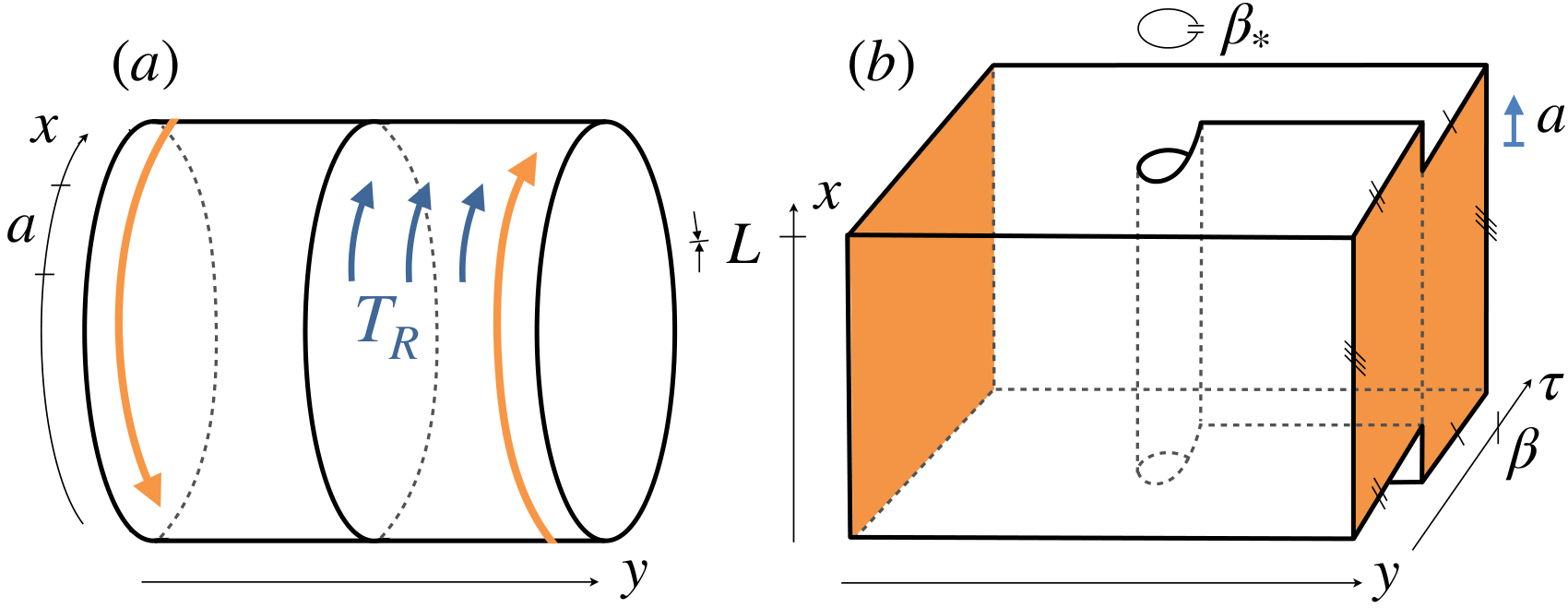
Following Ref.[212], we define , which is related to the usual partition function (), by the insertion of the operator , which translates the right half of the cylinder by one unit cell in the periodic direction, see Fig.7(a). The object satisfies
| (4.2) |
where is the number of sites in the direction, is non-universal and has a negative real part, and indicates corrections that decay faster than as . The above expression is valid at temperatures low compared to the finite-size energy differences on the boundary, , see Appendix K.
Equation (4.2) follows analytically from the low energy description of chiral topological matter in terms of chiral TFT and CFT [212], and was numerically scrutinized in a large number of examples in Refs.[212, 213, 38, 61, 214], as well as in Appendix L. Nevertheless, we are not aware of a rigorous proof of Eq.(4.2) for gapped lattice Hamiltonians. Therefore, in stating our results we will use the assumption ’the Hamiltonian is in a chiral topological phase of matter’, the content of which is that admits a low energy description in terms of a chiral TFT with chiral central charge and topological spins , and in particular, Eq.(4.2) holds for any bulk-gap preserving deformation of , with (apart from accidental degeneracies on the cylinder, as explained below Eq.(4.1)). In the remainder of this section we further discuss the content of Eq.(4.2) and its expected range of validity, in light of the Hamiltonian and space-time interpretations of .
From a Hamiltonian perspective, is the thermal expectation value of , evaluated at a temperature low enough to isolate the ground state. The exponential decay expressed in Eq.(4.2) appears because is not a symmetry of , and can be understood as the energy density of the line defect where is discontinuous, see Fig.7(a). In fact, we expect Eq.(4.2) to hold irrespective of whether the uniform translation is a symmetry of , or of the underlying ’lattice’ on which is defined, which may be any polygonalization of the cylinder (see Ref.[266] for a similar scenario). The only expected requirement is that the low energy description of is homogeneous. Furthermore, if Eq.(4.2) only holds after a disorder averaging of , our results and derivations in the following sections remain unchanged.
There is also a simple space-time interpretation of , which will be useful in the context of DQMC. The usual partition function has a functional integral representation in terms of bosonic fields (fermionic fields ) defined on space, the cylinder in our case, and the imaginary time circle , with periodic (anti-periodic) boundary conditions [267]. In , the insertion of produces a twisting of the boundary conditions of in the time direction, such that is the partition function on a space-time carrying a screw dislocation, see Fig.7(b).
The above interpretation of , supplemented by Eq.(4.1), allows for an intuitive explanation of Eq.(4.2), which loosely follows its analytic derivation [212]. As seen in Fig.7(b), the line where is discontinuous can be interpreted as an additional boundary component at a high effective temperature, . Since the effective temperature is much larger than the finite size energy-differences on the boundary CFT, the screw dislocation contributes no finite size corrections to . This leaves only the contribution of the boundary component on the right side of the cylinder, where produces the phase , assuming . Equation (4.1) then leads to the universal finite size correction .
4.2 Excluding stoquastic Hamiltonians for chiral topological matter
In this section we consider bosonic (or ’qudit’, or spin) systems, and a single design principle - existence of a local basis in which the many-body Hamiltonian is stoquastic. A sketch of the derivation of Result 1 is that the momentum polarization is positive for Hamiltonians which are stoquastic in an on-site and homogenous basis, and this implies that for any Hamiltonian obtained from by conjugation with a local unitary.
4.2.1 Setup
The many body Hilbert space is given by , where the tensor product runs over the sites of a 2-dimensional lattice , and are on-site ’qudit’ Hilbert spaces of finite dimension . With finite-size QMC simulations in mind, we consider a square lattice with spacing 1, sites, and periodic boundary conditions, so that is a discretization of the flat torus . Generalization to other 2-dimensional lattices is straight forward. On this Hilbert space a gapped -local Hamiltonian is assumed to be given. Here the terms are supported within a range of - they are defined on and act as the identity on all other qudits.
Fix an tensor product basis , labeled by strings , where labels a basis for . For any vector , the corresponding translation operator is defined in this basis, , with . These statements assert that is both an on-site and a homogeneous basis, or on-site homogenous for short. Note that acts as a permutation matrix on the s, and in particular, has non-negative matrix elements in this basis.
In accordance with Sec.4.1.2, we assume that the low energy description of is invariant under , as defined above. In doing so, we exclude the possibility of generic background gauge fields for any on-site symmetry that may posses, which is beyond the scope of this thesis. Nevertheless, commonly used background gauge fields, such as those corresponding to uniform magnetic fields with rational flux per plaquette, can easily be incorporated into our analysis, by restricting to translation vectors in a sub-lattice of . A restriction to sub-lattice translations can also be used to guarantee that acts purely as a translation in the low energy TQFT description. In particular, a lattice translation may permute the anyon types 2929 29 We thank Michael Levin for pointing out this phenomenon.. Since the number of anyons is finite, restricting to large enough translations will eliminate this effect. An example is given by Wen’s plaquette model, where different anyons are localized on the even/odd sites of a bipartite lattice [268], and a restriction to translations that maps the even (odd) sites to themselves will be made.
Finally, we assume that is locally stoquastic: it is term-wise stoquastic in a local basis. This means that a local unitary operator exists, such that the conjugated Hamiltonian is a sum of local terms , which have non-positive matrix elements in the on-site homogeneous basis, for all basis states . Note that we include the diagonal matrix elements in the definition, without loss of generality.
The term local unitary used above refers to a depth- quantum circuit, a product where each is itself a product of unitary operators with non-overlapping supports of diameter . It follows that has a range , where is the range of . Equivalently, we may take to be a finite-time evolution with respect to an -local, smoothly time-dependent, Hamiltonian , given by the time-ordered exponential . The two types of locality requirements are equivalent, as finite-time evolutions can be efficiently approximated by finite-depth circuits, while finite-depth circuits can be written as finite-time evolutions over time with piecewise constant -local Hamiltonians [269, 90].
4.2.2 Constraining and
In order to discuss the momentum polarization, we need to map the stoquastic Hamiltonian from the torus to a cylinder . This is done by choosing a translation vector , and then cutting the torus along a line parallel to . To simplify the presentation we restrict attention to the case , where (and in the following ). All other cases amount to a lattice-spacing redefinition, see Appendix M. The cylinder is then obtained from the torus by cutting along the line . A stoquastic Hamiltonian on the cylinder can be obtained from that on the torus by removing all local terms whose support overlaps , see Fig.8. Note that this procedure may render acting as on certain qudits with within a range of , but this does not bother us. Since all terms are individually stoquastic, this procedure leaves , now defined on the cylinder, stoquastic. One can similarly map and to the cylinder such that the relation remains valid on .

Let us now make contact with the momentum polarization Eq.(4.2). Having mapped to the cylinder, we consider the ’partition function’
| (4.3) |
where is defined by , , and is a heavy side function supported on the right half of the cylinder. Though is generally different from appearing in Eq.(4.2), it satisfies two useful properties:
- 1.
. Both and have non-negative entries in the on-site basis , and therefore so does .
- 2.
is in the same phase of matter as , so and . Moreover, for all . Treating as a finite time evolution, we have , where , as a deformation from to which maintains locality and preserves the bulk-gap. Moreover, the full spectrum on the cylinder is -independent, and therefore so is .
Combining Eq.(4.2), for instead of , with the two above properties leads to
| (4.4) | ||||
where is generally different from of Eq.(4.2) since . The non-universal integer part of can then be eliminated by raising Eq.(4.4) to the th power,
| (4.5) |
where we used , and as . We also indicated explicitly the possible -dependence of , as described in Sec.4.1.1. We proceed under the assumption that no accidental degeneracies occur on the cylinder, so that for all , deferring the degenerate case to Appendix N. Now, for rational , the series () covers periodically a subset of the th roots of unity, including . On the other hand, for irrational the series is dense in the unit circle. Combined with the fact that is valued in the finite set , while is -independent, Equation (4.5) implies that must be rational, and that the values attained by cover the set periodically, for large enough . It follows that . We therefore have
- Result 1
-
If a local bosonic Hamiltonian is both locally stoquastic and in a chiral topological phase of matter, then one of the corresponding topological spins satisfies . Equivalently, a bosonic chiral topological phase of matter where is not the topological spin of some anyon, i.e , admits no local Hamiltonians which are locally stoquastic.
The above result can be stated in terms of the topological -matrix, which is the representation of a Dehn twist on the torus ground state subspace, and has the spectrum [218, 104, 213, 212, 98, 270].
- Result 1’
-
If a local bosonic Hamiltonian is is both locally stoquastic and in a chiral topological phase of matter, then the corresponding -matrix satisfies . Equivalently, a bosonic chiral topological phase of matter where , admits no local Hamiltonians which are locally stoquastic.
The above result is our main statement for bosonic phases of matter. The logic used in its derivation is extended in Sec.4.3-4.5, where we generalize Result 1 to systems which are fermionic, spontaneously-chiral, or both.
4.3 Spontaneous chirality
The invariants and change sign under both time reversal and parity (spatial reflection) , and therefore require a breaking of and down to to be non-vanishing. The momentum polarization Eq.(4.2) is valid if this symmetry breaking is explicit, i.e does not commute with and separately. Here we consider the case where is -symmetric, but these are broken down to spontaneously, as in e.g intrinsic topological superfluids and superconductors [27, 2, 271]. We first generalize Eq.(4.2) to this setting, and then use this generalization to obtain a spontaneously-chiral analog of Result 1.
Note that the physical time-reversal is an on-site anti-unitary operator acting identically on all qudits, which implies , while is a unitary operator that maps the qudit at to that at , where is the nontrivial element in , e.g .
4.3.1 Momentum polarization for spontaneously-chiral Hamiltonians
For simplicity, we begin by assuming that is ’classically symmetry breaking’ - it has two exact ground states on the cylinder, already at finite system sizes. We therefore have two ground states , such that is obtained from by acting with either or . In particular, have opposite values of and . The density matrix is then , where , and this modifies the right hand side of Eq.(4.2) to its real part,
| (4.6) | ||||
where are the values of the non-universal obtained from Eq.(4.2), by replacing by . Indeed, it follows from that if two density matrices are related by , then are complex conjugates, .
Now, for a generic symmetry breaking Hamiltonian , exact ground state degeneracy happens only in the infinite volume limit [272]. At finite size, the two lowest lying eigenvalues of would be separated by an exponentially small energy difference , with some . The two corresponding eigenstates would be -even/odd, of the form , where is a -invariant local unitary [90]. One can think of these statements as resulting from the existence of a bulk-gap preserving and -symmetric deformation of to a ’classically symmetry breaking’ Hamiltonian3030 30 The canonical example is the transverse field Ising model in 1+1d. Exact ground state degeneracy appears at finite only for , though spontaneous symmetry breaking occurs for all , where a splitting appears..
In the generic setting, we have
| (4.7) |
and, following our treatment of the local unitary in the previous section, Equation (4.6) remains valid, with modified , but unchanged . This statement holds for temperatures much higher than and much smaller that the CFT energy spacing, , or more accurately and (cf. Sec.4.1.2). Note that the universal content of Eq.(4.6) is the absolute value , since the cosine is even and is non-universal.
4.3.2 Constraining and
Let us now assume that a gapped and local Hamiltonian is ,-symmetric, and is locally stoquastic, due to a unitary . It follows that , where . If happens to be ,-symmetric, then so is , and Eq.(4.6) holds for , with in place of . For a general , we have
| (4.8) |
where need not be ,-symmetric. As result, satisfies a weaker form of Eq.(4.6),
| (4.9) |
where may differ from , and we also indicated the positivity of . Now, if , one of the chiral contributions is exponentially suppressed relative to the other as , and we can apply the analysis of Sec.4.2. If , we obtain
| (4.10) |
in analogy with Eq.(3.3).Unlike Eq.(3.3), taking the th power of this equation does not eliminate the mod 1 ambiguity in . This corresponds to the fact that, as opposed to explicitly chiral systems, stacking copies of a spontaneously chiral system does not increase its net chirality. One can replace in with a larger half-translation , which would multiply the argument of the cosine by . However, since the largest translation on the cylinder is obtained for , this does not eliminate the mod 1 ambiguity in . Moreover, even if it so happens that , Equation (4.10) does not imply (mod 1) since is large.
In order to make progress, we make use of the bagpipes construction illustrated in Fig.9. We attach identical cylinders, or ’pipes’, to the given lattice, and act with on these cylinders. The global topology of the given lattice is unimportant - all that is needed is a large enough disk in which the construction can be applied. The construction does require some form of homogeneity in order to have a unique extension of the Hamiltonian to the pipes, and which will be identical for all pipes. We will assume a strict translation symmetry with respect to a sub-lattice, but we believe that this assumption can be relaxed.

The resulting surface, shown in Fig.9, has negative curvature at the base of each pipe, which requires a finite number of lattice disclinations in this region. In order to avoid any possible ambiguity in the definition of at a disclination, one can simply remove any local term whose support contains a disclination, which amounts to puncturing a hole around each disclination. The resulting boundary components do not contribute to the momentum polarization since acts on these as the identity.
With the construction at hand, the identical contributions of all cylinders to add, which implies
| (4.11) |
Setting gives
| (4.12) | ||||
where we indicate explicitly the possible -dependence of . This is the spontaneously chiral analog of Eq.(4.5), and can be analyzed similarly. Since is valued in the finite set , both must be rational, . Restricting then to , such that , and attains a constant value for large enough , we have
| (4.13) |
for some anyon . Repeating the analysis with times more pipes , replaces in Eq.(4.13) with its th power, for all . This infinite set of equations then implies . To summarize,
- Result 2
-
If a local bosonic Hamiltonian is both locally stoquastic and in a spontaneously-chiral topological phase of matter, then one of the corresponding topological spins satisfies . Equivalently, a bosonic spontaneously-chiral topological phase of matter where is not the topological spin of some anyon, i.e , admits no local Hamiltonians which are locally stoquastic.
This extends Result 1 beyond explicitly-chiral Hamiltonians, and clarifies that the essence of the intrinsic sign problem we find is the macroscopic, physically observable, condition , as opposed to the microscopic absence (or presence) of time reversal and reflection symmetries.
4.4 DQMC: locality, homogeneity, and geometric manipulations
In order to obtain fermionic analogs of the bosonic results of the previous sections, we first need to establish a framework in which such results can be obtained. In this section we develop a formalism that unifies and generalizes the currently used DQMC algorithms and design principles, and implement within it the geometric manipulations used in previous sections, in a sign-free manner. Since we wish to treat the wide range of currently known DQMC algorithms and design principles on equal footing, the discussion will be more abstract than the simple setting of locally stoquastic Hamiltonians used above. In particular, Sections 4.4.1-4.4.2 lead up to the definition of locally sign-free DQMC, which is our fermionic analog of a locally stoquastic Hamiltonian. This definition is used later on in Sec.4.5 to formulate Result 1F and Result 2F, the fermionic analogs of Results 1 and 2. The new tools needed to establish these results are the sign-free geometric manipulations described in Sec.4.4.4.
4.4.1 Local DQMC
In the presence of bosons and fermions, the many-body Hilbert space is given by , where is a fermionic Fock space, equipped with an on-site occupation basis , , generated by acting with fermionic (anti-commuting) creation operators on the Fock vacuum . The product is taken with respect to a fixed ordering of fermion species and lattice sites . We will also make use of the single-fermion space , spanned by , where is the system size. As in Sec.4.2, is a many-qudit Hilbert space with local dimension . It can also be a bosonic Fock space where .
We consider local fermion-boson Hamiltonians , of the form
| (4.14) |
where the free-fermion Hermitian matrix is -local, it vanishes unless , and we suppress, here and in the following, the fermion species indices. The Hamiltonian describes all possible -local interactions which preserve the fermion parity , where , including fermion-independent terms as in Sec.4.2. Thus is of the form
| (4.15) | ||||
where (for all ) is a local bosonic operator with range , and vanishes unless , and similarly for , which vanishes unless are contained in a disk or radius . In Eq.(4.15) dots represent additional pairing terms of the form , , or , , as well as terms with a higher number of fermions, all of which are -local and preserve the fermion parity.
Since locality is defined in terms of anti-commuting Fermi operators, a local stoquastic basis is not expected to exist, and accordingly, the sign problem appears in any QMC method in which the Boltzmann weights are given in terms of Hamiltonian matrix elements in a local basis [72, 71]. For this reason, the methods used to perform QMC in the presence of fermions are distinct from the ones used in their absence. These are collectively referred to as DQMC [206, 65, 77, 71, 70], and lead to the imaginary time path integral representation of the partition function ,
| (4.16) | ||||
involving a bosonic field with an action , and a fermionic (grassmann valued) field , with a quadratic action defined by the -dependent single-fermion operator . In the third line of Eq.(4.16) we assumed the Hamiltonian form , and used a standard identity for the determinant in terms of the single-fermion imaginary-time evolution operator [206], where TO denotes the time ordering. The field () is defined on a continuous imaginary-time circle , with periodic (anti-periodic) boundary conditions, and on the spatial lattice . The second and third lines of Eq.(4.16) define the Monte Carlo phase space and Boltzmann weight
| (4.17) | ||||
In applications, the DQMC representation (4.16) may be obtained from the Hamiltonian in a number of ways. If a Yukawa type model is assumed as a starting point [70], i.e , then the action is obtained from the Hamiltonian , and . Alternatively, the representation (4.16) may be obtained through a Hubbard-Stratonovich decoupling and/or a series expansion of fermionic self-interactions [273, 207, 205]. Such is the case e.g when there are no bosons , and . Note that for a given fermionic self-interaction, there are various possible DQMC representations, obtained e.g via a Hubbard-Stratonovich decoupling in different channels.
To take into account and generalize the above relations between and the corresponding DQMC representation, we will only assume (i) that the effective single-fermion Hamiltonian reduces to the free fermion matrix in the absence of , i.e , (ii) that the boson field is itself an -local object3131 31 Thus is a map from sets of lattice sites with diameter less than , such as links, plaquettes etc., to a fixed vector space . Additionally, the integration in (4.16) runs over all such functions. As an example, restricting to constant functions leads to non-local all to all interactions between fermions., and (iii) that the -locality of and implies the -locality of and , where is some function of , independent of system size. The physical content of these assumptions is that the fields and operators correspond to the same physical fermion3232 32 Technically, via the fermionic coherent state construction of the functional integral [267]., and that the boson mediates all fermionic interactions , and therefore corresponds to both the physical bosons in and to composite objects made of an even number of fermions within a range (e.g a Cooper pair ).
We can therefore write
| (4.18) | ||||
where each term depends only on the values of at points with , and similarly, each term is supported on a disk of radius around , and depends on the values of at points within this disk.
Note that even though is Hermitian, we do not assume the same for . Non-Hermitian s naturally arise in Hubbard–Stratonovich decouplings, see e.g [274, 205]. Even when is Hermitian for all , its time-dependence implies that is non-Hermitian, and therefore in Eq.(4.17) is generically complex valued [206]. This is the generic origin of the sign problem in DQMC. Section 4.4.2 below describes the notion of fermionic design principles, algebraic conditions on implying , and defines what it means for such design principles to be local and homogenous.
In the following analysis, we exclude the case of ’classically-interacting fermions’, where is time-independent and is Hermitian. In this case the fermionic weight is trivially non-negative, and sign-free DQMC is always possible, provided . We view such models as ’exactly solvable’, on equal footing with free-fermion and commuting projector models. Given a phase of matter, the possible existence of exactly solvable models is independent of the possible existence of sign-free models. Even when an exactly solvable model exists, QMC simulations are of interest for generic questions, such as phase transitions due to deformations of the model [275]. In particular, Ref.[276] utilized a classically-free description of Kitaev’s honeycomb model to obtain the thermal Hall conductance and chiral central charge, which should be contrasted with the intrinsic sign problem we find in the corresponding phase of matter, see Table 1 and Sec.4.5.
4.4.2 Local and homogenous fermionic design principles
The representation (4.16) is sign-free if for all . A design principle then amounts to a set of polynomially verifiable properties 3333 33 That is, properties which can be verified in a polynomial-in- time. As an example, given a local Hamiltonian, deciding whether there exists a local basis in which it is stoquastic is NP-complete [73, 74]. In particular, one does not need to perform the exponential operation of evaluating on every configuration to assure that . Had this been possible, there would be no need for a Monte Carlo sampling of the phase space . of and that guarantee that the complex phase of is opposite to that of . For the sake of presentation, we restrict attention to the case where is manifestly real valued, and due to an algebraic condition on the operator , which we write as . This is assumed to follow from an algebraic condition on , written as , manifestly satisfied for all . The set is assumed to be closed under addition, while is closed under multiplication: for all , and for all .
The simplest example, where is the set of matrices obeying a fixed time reversal symmetry, is discussed in Sec.4.4.3. In Appendix P we review all other design principles known to us, demonstrate that most of them are of the simplified form above, and generalize our arguments to those that are not. Comparing with the bosonic Hamiltonians treated in Sec.4.2, we note that is analogous to the set of stoquastic Hamiltonians in a fixed basis, while is analogous to the resulting set of matrices with non-negative entries.
Design principles, as defined above (and in the literature), are purely algebraic conditions, which carry no information about the underlying geometry of space-time. However, as demonstrated in Sec.4.4.3, in order to allow for local interactions, mediated by an -local boson , a design principle must also be local in some sense. We will adopt the following definitions, which are shown to be satisfied by all physical applications of design principles that we are aware of, in Sec.4.4.3 and Appendix P.
Definition (term-wise sign-free):
We say that a DQMC representation is term-wise sign-free due to a design principle , if each of the local terms obey the design principle separately, rather than just they sums . Thus is real valued, and , for all .
This is analogous to the requirement in Sec.4.2.1 that be term-wise stoquastic. Note that even when a DQMC representation is term-wise sign-free, the resulting Boltzmann weights are sign-free in a non-local manner: involves the values of at all space-time points, and splitting the determinant into a product of local terms by the Leibniz formula reintroduces signs, which capture the fermionic statistics. In this respect, the “classical” Boltzmann weights are always non-local in DQMC.
Definition (on-site homogeneous design principle):
A design principle is said to be on-site homogenous if any permutation of the lattice sites obeys it. That is, the operator
| (4.19) |
viewed as a single-fermion imaginary-time evolution operator, obeys the design principle: , for all .
This amounts to the statement that the design principle treats all lattice sites on equal footing, since it follows that if and only if , for all permutations . It may be that a design principle is on-site homogeneous only with respect to a sub-lattice . In this case we simply treat as the spatial lattice, and add the finite set to the internal degrees of freedom. Comparing with Sec.4.2.1, on-site homogeneous design principles are analogous to the set of Hamiltonians which are stoquastic in an on-site homogeneous basis - any qudit permutation operator has non-negative entries in this basis, like the imaginary time evolution .
With these two notions of locality and homogeneity in design principles, we now define the DQMC analog of locally stoquastic Hamiltonians (see Sec.4.2).
Definition (locally sign-free DQMC):
Given a local fermion-boson Hamiltonian , we say that allows for a locally sign-free DQMC simulation, if there exists a local unitary , such that has a local DQMC representation (4.16), which is term-wise sign-free due to an on-site homogeneous design principle.
Note that the DQMC representation (4.16) is not of the Hamiltonian but of the partition function, and clearly . What the above definition entails, is that it is , rather than , from which the DQMC data is obtained, as described in Sec.4.4.1. This data is then assumed to be term-wise sign-free due to an on-site homogeneous design principle. The local unitary appearing in the above definition is generally fermionic [277]: it can be written as a finite time evolution , where is a local fermion-boson Hamiltonian, which is either piecewise-constant or smooth as a function of , c.f Sec.4.2.1.
4.4.3 Example: time reversal design principle
To demonstrate the above definitions in a concrete setting, consider the time-reversal design principle, defined by an anti-unitary operator acting on the single-fermion Hilbert space , such that . The set contains all -invariant matrices, . It follows that , so that in this case, and this implies [81, 274].
A sufficient condition on that guarantees that the design principle it defines is on-site homogenous is that it is of the form , where is the identity matrix on , and is an anti-unitary on that squares to . Equivalently, is block diagonal, with identical blocks corresponding to the lattice sites . It is then clear that the permutation matrices defined in Eq.(4.19) commute with , so for all . Note that the design principle may correspond to a physical time-reversal , discussed in Sec.4.3, only if it is on-site homogenous, which is why we distinguish the two in our notation.
Additionally, if the operator is -local with some range , then any local which is sign-free due to can be made term-wise sign-free. Indeed, if then
| (4.20) | ||||
where is now supported on a disk of radius and commutes with , for all . We see that the specific notion of -locality coincides with the general notion of ’term-wise sign free’. In particular, has a range , and can therefore be applied term-wise.
The above statements imply that if , where is a single-fermion local unitary, and has a local DQMC representation which is sign-free due to , then allows for a locally sign-free DQMC simulation. Indeed, extending to a many-body local unitary , we see that admits a local DQMC representation where . Since is on-site homogenous, and can be assumed term-wise sign-free (see Eq.(4.20)), we have the desired result. As demonstrated in Appendix P, much of the above analysis carries over to other known design principles.
All realizations of presented in Ref.[274] in the context of generalized Hubbard models, and in Ref.[70] in the context of quantum critical metals, have the on-site homogeneous form , and therefore correspond to locally sign-free DQMC simulations.
We now consider a few specific time-reversal design principles . The physical spin-1/2 time reversal , where , and correspond to up and down spin components, is an on-site homogeneous design principle, which accounts for the absence of signs in the attractive Hubbard model [274]. The composition of with a modulo 2 translation, , where is the even part of , is an on-site homogeneous design principle with respect to the sub-lattice, but not with respect to . On the other hand, the composition of with a spin-less reflection (or parity) , is not on-site homogeneous with respect to any sub-lattice.

The latter example is clearly non-local, and we use it to demonstrate the necessity of locality in design principles. As discussed in Sec.4.3, the breaking of and down to actually defines the notion of chirality, and therefore is a natural symmetry in chiral topological matter. Accordingly, the design principle applies to a class of models for chiral topological phases, see Appendix O. This seems to allow, from the naive algebraic perspective, for a sign-free DQMC simulation of certain chiral topological phases. However, the weights will only be non-negative for bosonic configurations which are is invariant under . Restricting the integration in Eq.(4.16) to such configurations leads to non-local interactions between fermions , coupling the points and . These interactions effectively fold the non-local chiral system into a local non-chiral system on half of space, see Fig.10. Thus, does not allow for sign-free DQMC simulations of chiral topological matter.
4.4.4 Sign-free geometric manipulations in DQMC
Let be a partition function in a local DQMC form (4.16), on the discrete torus and imaginary time circle , which is term-wise sign-free due to an on-site homogenous design principle. In this section we show that it is possible to cut to the cylinder , and subsequently introduce a screw dislocation in the space-time , which corresponds to the momentum polarization (4.2), while maintaining the DQMC weights non-negative.
Introducing spatial boundaries
Given a translation (), we can cut the torus along a line parallel to , and obtain a cylinder where acts as a translation within each boundary component, as in Sec.4.2. Given the DQMC representation (4.16) on , the corresponding representation on is obtained by eliminating all local terms whose support overlaps , as in Fig.8. This procedure may render independent of certain degrees of freedom , with within a range of , in which case we simply remove such degrees of freedom from the functional integral (4.16)3434 34 For -local , which is defined on links, plaquettes, etc., we also remove from the functional integration those links, plaquettes, etc. which overlap .. Since obey the design principle for every , the resulting still obey the design principle and the weights remain real and non-negative.
Introducing a screw dislocation in space-time
Let us now restrict attention to , and make contact with the momentum polarization (4.2). Given a partition function on the space-time , consider twisting the boundary conditions in the time direction,
| (4.21) | ||||
Note that , since . In particular, the full twist is equivalent to the untwisted case , which is equivalent to the statement that the modular parameter of the torus is defined mod 1 (see e.g example 8.2 of [234]). The case gives the standard boundary conditions, where the partition function is, in Hamiltonian terms, just . In this case since is Hermitian, though its QMC representation will generically involve complex valued weights . The twisted case includes the insertion of the half-translation operator
| (4.22) |
which appears in the momentum polarization (4.2). Since is unitary rather than hermitian, itself will generically be complex. However,
Claim:
If has a local DQMC representation (4.16), which is term-wise sign-free due to an on-site homogeneous design principle, then also has a sign-free QMC representation: , with . In particular, .
Proof of the claim is provided below. It revolves around two physical points: (i) For the boson , we only use the fact that all boundary conditions, and those in Eq.(4.21) in particular, are locally invisible. (ii) For the fermion , the local invisibility of boundary conditions does not suffice, and the important point is that translations do not act on internal degrees of freedom, and therefore correspond to permutations of the lattice sites. The same holds for the half translation . This distinguishes translations from internal symmetries, as well as from all other spatial symmetries, which involve point group elements, and generically act non-trivially on internal degrees of freedom. For example, a rotation will act non-trivially on spin-full fermions.
Proof:
We first consider the fermionic part of the Boltzmann weight, . The Hamiltonian depends on the values of at a single time slice , and is therefore unaffected by the twist in bosonic boundary conditions. It follows that is independent of the twist in bosonic boundary conditions. On the other hand, the fermionic boundary conditions in (4.21) correspond to a change of the time evolution operator , in analogy with (4.22). Since the design-principle is assumed to be on-site homogeneous, and is a permutation operator, with , we have , and .
Let us now consider the bosonic part of the Boltzmann weight , where each of the local terms is manifestly real valued for all . We assume that the imaginary time circle is discretized, such that the total number of space-time points is finite. Such a discretization is common in DQMC algorithms [206, 207], and the continuum case can be obtained by taking the appropriate limit. The term can then be written as a composition , where is a real valued function, and chooses the values of on which depends, where is the support of . The bosonic boundary conditions (4.21) then amount to a modification of the support , as depicted in Fig.11, but not of the function , which remains real valued. In particular, for we have , and .
Combining the above conclusions for the bosonic and fermionic parts of , we find that for all .

4.5 Excluding sign-free DQMC for chiral topological matter
We are now ready to demonstrate the existence of an intrinsic sign problem in chiral topological matter comprised of bosons and fermions, using the machinery of Sections 4.2-4.4.
Let be a gapped local fermion-boson Hamiltonian on the discrete torus, which allows for a locally sign-free DQMC simulation. Unpacking the definition, this means that has a local DQMC representation which is term-wise sign-free due to an on-site homogeneous design principle. As shown in Sec.4.4.4, this implies that , written on the cylinder, also has a local DQMC representation, obeying a local and on-site design principle, and as a result, . Now, as shown in Sec.4.2, the positivity of implies for some anyon . We therefore have the fermionic version of Result 1,
- Result 1F
-
If a local fermion-boson Hamiltonian , which is in a chiral topological phase of matter, allows for a locally sign-free DQMC simulation, then one of the corresponding topological spins satisfies . Equivalently, a chiral topological phase of matter where is not the topological spin of some anyon, i.e , admits no local fermion-boson Hamiltonians for which locally sign-free DQMC simulation is possible.
As shown in Sec.4.3, the positivity of implies for some anyon , even if chirality appears only spontaneously. We therefore obtain the fermionic version of Result 2,
- Result 2F
-
If a local fermion-boson Hamiltonian , which is in a spontaneously-chiral topological phase of matter, allows for a locally sign-free DQMC simulation, then one of the corresponding topological spins satisfies . Equivalently, a spontaneously-chiral topological phase of matter where is not the topological spin of some anyon, i.e , admits no local fermion-boson Hamiltonians which allow for a locally sign-free DQMC simulation.
In stating these results, we do not restrict to fermionic phases, because bosonic phases may admit a fermionic description, for which DQMC is of interest. When a bosonic phase admits a fermionic description, the bosonic field in Eq.(4.16) will contain a gauge field that couples to the fermion parity of . An important series of examples is given by the non-abelian Kitaev spin liquids, which admit a description in terms of gapped Majorana fermions with an odd Chern number , coupled to a gauge field [104]. As described in Table 1, the criterion applies to the Kitaev spin liquid, for all . Result 1 then excludes the possibility of locally stoquastic Hamiltonians for the microscopic description in terms of spins, while Result 1F excludes the possibility of locally sign-free DQMC simulations in the emergent fermionic description.
4.6 Conjectures: beyond chiral matter
In Sec.4.2 and Appendices 4.3-4.5 we established a criterion for the existence of intrinsic sign problems in chiral topological matter: if , or equivalently (see Result 1’), then an intrinsic sign problem exists. Even if taken at face value, this criterion never applies to non-chiral bosonic topological phases, where , due to the vacuum topological spin . The same statement applies to all bosonic phases with . In this section we propose a refined criterion for intrinsic sign problems in topological matter, which non-trivially applies to both chiral and non-chiral cases, and also unifies the results of this section with those obtained by other means in a parallel work [5].
Reference [266] proposed the ’universal wave-function overlap’ method for characterizing topological order from any basis for the ground state subspace of a local gapped Hamiltonian on the torus . The method is based on the conjecture
| (4.23) |
where is the area of the torus, is a non-universal complex number with non-negative real part, the microscopic Dehn-twist operator implements the Dehn twist on the Hilbert space, and are the entries of the topological -matrix that characterizes the phase of , in the basis . The same statement applies to any element of the mapping class group of the torus, isomorphic to , with in place of in Eq.(4.23). The non-universal exponential suppression of the overlap is expected because will not generically map the ground-state subspace to itself, but if happens to be a symmetry of , then [278, 98]. Though we are not aware of a general analytic derivation of Eq.(4.23), it was verified analytically and numerically in a large number of examples in Refs.[266, 270, 279, 280, 281], for Hamiltonians in both chiral and non-chiral phases.
Note the close analogy between Eq.(4.23) and the momentum polarization (4.2), where the microscopic Dehn-twist on the torus and the half translation on the cylinder play a similar role, and non-universal extensive contributions are followed by sub-extensive universal data. To make this analogy clearer, and make contact with the analysis of Sections 4.2 and 4.5, we consider the object , which satisfies
| (4.24) |
and can be interpreted as either the (unnormalized) thermal expectation value of , or the partition function on a space-time twisted by , in analogy with Sec.4.1.2. Equation (4.24) is valid for temperatures , much lower than the bulk gap and much higher than any finite size splitting in the ground state-subspace, .
Just like , the operator acts as a permutation of the lattice sites. Therefore, following Section 4.2 and Appendix 4.5, if is either locally stoquastic, or admits a locally sign-free DQMC simulation, then . In terms of and , this implies , where the sum runs over all topological spins.
The last statement applies to both bosonic and fermionic Hamiltonians. For bosonic Hamiltonians, it can be strengthened by means of the Frobenius-Perron theorem. If is stoquastic in the on-site basis , Hermitian, and has a degenerate ground state subspace, then this subspace can be spanned by an orthonormal basis with positive entries in the on-site basis, , see e.g Ref.[5]. This implies that
| (4.25) |
where is generally different from , but the matrix has the same spectrum as in Eq.(4.23). This is a stronger form of (J.18), which implies . Since is also unitary, it is a permutation matrix, for some , where is the number of ground states. In turn, this implies that the spectrum of is a disjoint union of complete sets of roots of unity,
| (4.26) |
where is the set of th roots of unity, , and . Therefore,
- Conjecture 1
-
A bosonic topological phase of matter where is not a disjoint union of complete sets of roots of unity, admits no local Hamiltonians which are locally stoquastic.
In particular, this implies an intrinsic sign problem whenever , thus generalizing Result 1. Moreover, the above statement applies non-trivially to phases with . In particular, for non-chiral phases, where , it reduces to the result established in Ref.[5], thus generalizing it as well. The simplest example for a non-chiral phase with an intrinsic sign problem is the doubled semion phase, where [211].
Though we are currently unaware of an analog of the Frobenius-Perron theorem that applies to DQMC, we expect that an analogous result can be established for fermionic Hamiltonians.
- Conjecture 1F
-
A topological phase of matter where is not a complete set of roots of unity, admits no local fermion-boson Hamiltonians for which locally sign-free DQMC simulation is possible.
The above conjectures suggest a substantial improvement over the criterion . To demonstrate this, we go back to the Laughlin phases and Chern-Simons theories considered in Table 1. We find a conjectured intrinsic sign problem in all of the first one-thousand bosonic Laughlin phases ( even), fermionic Laughlin phases ( odd), and Chern-Simons theories. In particular, we note that the prototypical Laughlin phase is not captured by the criterion , but is conjectured to be intrinsically sign-problematic.
4.7 Discussion
In this section we established the existence of intrinsic sign problems in a broad class of chiral topological phases, namely those where does not happen to be the topological spin of an anyon. Since these intrinsic sign problems persist even when chirality appears spontaneously, they are rooted in the macroscopic and observable data , , rather than the microscopic absence (or presence) of time reversal symmetry. Going beyond the simple setting of stoquastic Hamiltonians, we provided the first treatment of intrinsic sign problems in fermionic systems. In particular, we constructed a general framework which describes all DQMC algorithms and fermionic design principles that we are aware of, including the state of art design principles [205, 209, 208, 210] which are only beginning to be used by practitioners. Owing to its generality, it is likely that our framework will apply to additional design principles which have not yet been discovered, insofar as they are applied locally. We also presented conjectures that strengthen our results, and unify them with those obtained in Refs.[75, 5], under a single criterion in terms of and . These conjectures also imply intrinsic sign problems in many topological phases not covered by existing results.
Conceptually, our results show that the sign problem is not only a statement of computational complexity: it is, in fact, intimately connected with the physically observable properties of quantum matter. Such a connection has long been heuristically appreciated by QMC practitioners, and is placed on a firm and quantitative footing by the discovery of intrinsic sign problems. Despite the progress made here, our understanding of intrinsic sign problems is still in its infancy, and many open questions remain:
Quantum computation and intrinsic sign problems
Intrinsic sign-problems relate the physics of topological phases to their computational complexity, in analogy with the classification of topological phases which enable universal quantum computation [219, 97]. As we have seen, many phases of matter that are known to be universal for quantum computation are also intrinsically sign-problematic, supporting the paradigm of ’quantum advantage’ or ’quantum supremacy’ [220]. Determining whether intrinsic sign-problems appear in all phases of matter which are universal for quantum computation is an interesting open problem. Additionally, we identified intrinsic sign problems in many topological phases which are not universal for quantum computation. The intermediate complexity of such phases between classical and quantum computation is another interesting direction for future work.
Unconventional superconductivity and intrinsic sign problems
As described in the introduction, a major motivation for the study of intrinsic sign problems comes from long standing open problems in fermionic many-body systems, the nature of high temperature superconductivity in particular. It is currently believed that many high temperature superconductors, and the associated repulsive Hubbard models, are non-chiral -wave superconductors [80, 70], in which we did not identify an intrinsic sign problem. The optimistic possibility that the sign problem can in fact be cured in repulsive Hubbard models is therefore left open, though this has not yet been accomplished in the relevant regime of parameters, away from half filling, despite intense research efforts [79]. Nevertheless, the state of the art DMRG results of Ref.[80] do not exclude the possibility of a chiral -wave superconductor ( in Table 1). In this case we do find an intrinsic sign problem, which would account for the notorious sign problems observed in repulsive Hubbard models. More speculatively, it is possible that the mere proximity of repulsive Hubbard models to a chiral -wave phase stands behind their notorious sign problems. The possible effect of an intrinsic sign problem in a given phase on the larger phase diagram was recently studied in Ref.[282]. There is also evidence for chiral -wave superconductivity in doped graphene and related materials [283, 284], and our results therefore suggest the impossibility of sign-free QMC simulations of these. We believe that the study of intrinsic sign problems in the context of unconventional superconductivity is a promising direction for future work.
Non-locality as a possible route to sign-free QMC
The intrinsic sign problems identified in this thesis add to existing evidence for the complexity of chiral topological phases - these do not admit local commuting projector Hamiltonians [56, 57, 58, 54], nor do they admit local Hamiltonians with a PEPS state as an exact ground state [60, 61, 62, 63]. Nevertheless, relaxing the locality requirement does lead to positive results for the simulation of chiral topological matter using commuting projectors or PEPS. First, commuting projector Hamiltonians can be obtained if the local bosonic or fermionic degrees of freedom are replaced by anyonic (and therefore non-local) excitations of an underlying chiral topological phase [59]. Second, chiral topological Hamiltonians can have a PEPS ground state if they include interactions (or hopping amplitudes) that slowly decay as a power-law with distance. One may therefore hope that sign-free QMC simulations of chiral topological matter can also be performed if the locality requirements made in Sec.4.2 are similarly relaxed. Do such ’weakly-local’ sign-free models exist?
Easing intrinsic sign problems
In this section we proved the existence of an intrinsic sign problem in chiral topological phases of matter, but we did not quantify the severity of this sign problem, which is an important concept in both practical applications and theory of QMC. The severity of a sign problem is quantified by the smallness of the average sign of the QMC weights with respect to the distribution , i.e . Since can be viewed as the ratio of two partition functions, it obeys the generic scaling , with , as [72, 203]. A sign problem exists when , in which case QMC simulations require exponential computational resources, and this is what the intrinsic sign problem we identified implies for ’most’ chiral topological phases of matter. From the point of view of computational complexity, all that matters is whether or , but for practical applications the value of is very important, see e.g [283]. One may hope for a possible refinement of our results that provides a lower bound for , but since we have studied topological phases of matter, we view this as unlikely. It may therefore be possible to obtain fine-tuned models and QMC methods that lead to a small enough to be practically useful. More generally, it may be possible to search for such models and methods algorithmically, thus easing the intrinsic sign problem [203, 285, 286, 287]. We also note that the results presented in this thesis do not exclude approaches to the sign-problem based on a modified or constrained Monte Carlo sampling [204, 288, 289], as well as machine-learning aided QMC [290], and infinite-volume diagrammatic QMC [291].
Possible extensions
The chiral central charge only appears modulo 24 in our results. Nevertheless, for full value of is physically meaningful, as reviewed in the introduction. Does an intrinsic sign problem exist in all phases with ? The results of Ref.[76] strongly suggest this.
The arguments of Appendix 4.6 apply equally well to any element of the modular group, rather than just the topological -matrix, implying that the spectrum of all elements decomposes into full sets of roots of unity. Does this imply a tighter constraint on the TFT data than conjectured in Appendix 4.6? Moreover, the ’universal wave-function overlap’ conjecture, on which Appendix 4.6 relies, applies also to space-time dimensions , which suggests intrinsic sign problems in these space-time dimensions, including the beloved .
Another promising direction involves symmetry protected or enriched topological phases. In particular, the sign problem was cured in a number of bosonic SPT Hamiltonians [292, 293, 294, 295], and all SPT ground states can, by definition, be made non-negative in a local basis. Nevertheless, a ‘symmetry protected’ intrinsic sign problem, where symmetric local bases are excluded, was recently discovered [296]. Such constraints may be more useful for designing sign-free models than the stronger intrinsic sign problems discussed in this thesis.
5 Outlook
In this thesis we studied the geometric physics of chiral topological phases, and related this physics to the complexity of simulating such phases using quantum Monte Carlo algorithms. The analysis in Sec.2-3 was focused on chiral superfluids and superconductors, and revealed an intricate interplay of symmetry breaking, topology, and geometry. Though we stressed the Higgs mode as an emergent geometry in the relativistic analysis of Sec.2, the fuller non-relativistic treatment in Sec.3 was carried out at energy scales below the Higgs mass, where the emergent geometry simply follows the background geometry (or strain). We believe that there is beautiful physics to be revealed at higher energy scales, where the dynamics of the Higgs mode will be described by a non-relativistic, parity odd, and in part topological, quantum geometry similar to the Girvin-MacDonald-Platzman (GMP) mode in fractional quantum Hall states [297, 29, 30, 33, 45]. In particular, this physics should be important near a nematic phase transition where the spin-2 Higgs mode becomes light, which can be tuned by attractive Landau interactions [145]. We also believe that, through ‘composite fermions’ [15, 147, 148], this will lead to a new description of the GMP mode in paired quantum Hall states, including the illusive particle-hole invariant Pfaffian, and in analogy with the treatment of the GMP mode in Jain states close to half filling [298, 299, 300, 301].
Regarding intrinsic sign problems, we believe that the results obtained in Sec.4, as well as in Refs.[75, 76, 5, 296], represent the tip of an iceberg. Concrete extensions of these results were proposed in Sec.4.7. Beyond these, are there intrinsically sign-problematic phases which are not gapped, not topological, or both? Does the physics of high temperature superconductivity, or of dense nuclear matter, imply an intrinsic sign problem, thus accounting for the persistent sign problems observed by QMC practitioners in relevant models? Taking a broader perspective, intrinsic sign problems form a bridge between the notions of phases of matter and computational complexity. This should be contrasted with most results in quantum complexity [302, 303], which are established for classes of Hamiltonians defined by microscopic conditions such as locality, non-frustration, and stoquasticity, as well as energy gap assumptions, or for specific canonical models, but usually not for phases of matter. In fact, refining statements in quantum complexity to the level of phases was the original motivation for the study of intrinsic sign problems [75]. Additional statements regarding the complexity of phases are given by the classification of topological phases which enable universal quantum computation by anyon braiding [219, 97], and the proof that whenever the area law for entanglement entropy holds for a gapped Hamiltonian, it holds in its entire phase [304]. We find this theme to be promising for both the study of many-body quantum systems, and their use as computational devices.
Appendix
Appendix A Boundary fermions and gravitational anomaly
It is well known that the -wave SC has localized degrees of freedom on curves in space where the Chern number jumps, due to boundaries, or domain walls in or , which at low energies are chiral Majorana spinors [15]. In this section we derive the action for the boundary spinor in the presence of a space-time dependent order parameter, and describe its gravitational anomaly and corresponding anomaly inflow.
We start by deriving the boundary action in the geometric description in Appendix A.1, then review the relevant facts regarding the boundary gravitational anomaly within the gravitational description in Appendix A.2, and finally translate the results back to the -wave SC language in Appendix A.3.
The form of the boundary action in both the geometric description (A.8) and in the -wave SC language (A.23) is not surprising, and within the geometric description the gravitational anomaly and anomaly inflow are well known. It is the implication of gravitational anomaly and anomaly inflow for the -wave SC, through the emergent geometry described in sections 2.3 and 2.4, which is the result of this section.
A.1 Boundary fermions in a product geometry
We take the space time manifold to be , and assume that the vielbein has a product form with respect to the spatial coordinate ,
| (A.1) |
where and (unlike the notation of section 2.3 where ). To account for the orientation of the vielbein explicitly, we assumed has a positive orientation, and wrote . To be concrete we take for now. It follows that the metric also has the product form where . The form of the vielbein implies that the LC spin connection only has the nonzero components , which only depend on . We also assume that the spin connection only has nonzero components and depends only on . Under these assumptions , and therefore torsion simply drops out from the action, as can be seen from the form (B.8). This is a result of the low dimensionality of the problem. We further assume that the mass has the form of a flat domain wall in the direction. By this we mean with boundary conditions as , and , which corresponds to an interface between two distinct phases. To be concrete we take for now. then takes the form
| (A.2) |
This separable form implies the decomposition described in [305, 306], which we now apply to the present situation. Defining , the action takes the form
| (A.3) |
The operators and are hermitian and non negative. The positive parts of their spectrum coincide. We denote the positive eigenvalues by , including both the discrete and continuous parts of the spectrum, with the corresponding eigenfunctions satisfying . These eigenfunctions of are related by , where the sign chosen for is arbitrary, and for concreteness we take . Each set of eigenfunctions can be assumed to be orthonormal . Apart from the positive part of the spectrum, there can also be a unique eigenfunction with eigenvalue zero, a zero mode, for or but not both. The only candidates are , and a zero mode exists when one of these functions is normalizable. With our choice of boundary conditions for , only is normalizable. In terms of these eigenfunctions, the natural orthogonal decomposition of the spinor is
| (A.4) |
where are spinors of definite chirality, . Inserting this decomposition into (A.3) we obtain
| (A.5) | ||||
where . Thus the action splits into an infinite sum of actions for independent spinors, coupled to RC geometry, which in the case is the same as the coupling to Riemannian geometry. The spinor corresponding to the zero mode is chiral, massless, and exponentially localized on the domain wall as can be seen from the expression . It represents the robust boundary state that exists between two distinct topological phases. The chiral boundary spinor exhibits a gravitational anomaly, which we describe in the following.
All other spinors are non chiral and massive with masses . It is useful to think of the eigenvalue problems as one dimensional time independent Schrodinger problems to understand the eigenvalues and eigenfunctions [305, 306]. Almost all of the massive spinors correspond to delocalized bulk degrees of freedom, with the functions corresponding to “scattering states” of the “Hamiltonians” . Additionally, there can be a finite number of “bound states” , in which case corresponds to an additional non-chiral boundary state, which is not robust, and can always be removed by making the domain wall narrower, or the bulk masses smaller.
Since the action splits into a sum of fermionic actions and the decomposition (A.4) is orthogonal, the effective action also splits into a sum
| (A.6) |
where is the effective action obtained by integrating over a Majorana spinor with mass coupled to Riemannian geometry, and is the effective action obtained by integrating over a massless chiral Majorana spinor coupled to Riemannian geometry, with chirality . Above we assumed with and . Generalizing slightly, the net chirality of the boundary spinors is given by
| (A.7) |
The action for a single chiral Majorana spinor coupled to Riemannian geometry can be simplified by using a Majorana representation for the Clifford algebra, as described in appendix B.5.1. In the Majorana representation where is a single-component real Grassmann field and are the normalized eigenvectors of , . The action then reduces to
| (A.8) |
where .
A.2 Boundary gravitational anomaly and anomaly inflow
The chiral boundary spinor does not couple to the spin connection , and therefore does not distinguish the RC background from a Riemannian background described by the vielbein. This can be seen by examining the dimensional version of the conservation laws described in section 2.4.2 for the energy-momentum tensor and spin current of the boundary spinor. As in section 2.4.2, these follow from the and Lorentz gauge symmetries of the “classical” action . Since the boundary fermion does not couple to , its spin current vanishes, . Therefore (2.64) takes the form
| (A.9) |
expressing the symmetry of the boundary energy-momentum tensor, as in Riemannian geometry. The energy-momentum conservation law (2.70) then takes the form , which reduces to
| (A.10) |
where is the LC covariant derivative. This is the energy-momentum conservation law in a background Riemannian geometry. The energy-momentum tensor is given explicitly by
| (A.11) |
up to a term that vanishes on the equation of motion for , , which can also be written in a manifestly covariant form. One can verify that is conserved, symmetric, and traceless on the equation of motion.
Chiral Majorana fermions in coupled to Riemannian geometry exhibit a gravitational anomaly, which implies that while the “classical” action is invariant under both and Lorentz gauge transformations, the corresponding effective action is not 3535 35 is an example for the nonlocal boundary functional discussed in section 2.5.3.. A physical manifestation of this phenomena is that the “classical” conservation law is violated quantum mechanically, . The anomaly can be calculated by various techniques [12, 26], the simplest of which is the calculation of a single Feynman graph, as was originally done in [10] for the two dimensional Weyl spinor, and is reviewed in [26] part 5.1.2 for the case of a Majorana-Weyl spinor relevant here. The gravitational anomaly3636 36 There are a few ambiguities in describing what the gravitational anomaly is from an intrinsic boundary point of view. First, there is the issue of covariant versus consistent anomalies which also exists in gauge anomalies [12]. See also [25] and part 2 of [307] for a short review. Then, for the consistent gravitational anomaly, there is the issue of Lorentz anomalies versus Einstein () anomalies where one can obtain an effective boundary action that is invariant under local Lorentz transformations but not under , or vice versa [12]. It is also useful to discuss linear combinations of the Einstein and Lorentz anomalies, related to the symmetry of the effective action under the Lorentz-covariant action (2.68), see part 6.3 of [26]. All of these ambiguities are resolved when calculating the boundary energy-momentum tensor within the anomaly inflow mechanism: the bulk gCS term contributes to the boundary energy-momentum tensor, assuring it is symmetric and covariant, so that the physically relevant gravitational anomaly is the covariant Einstein anomaly [25], which is what we refer to here as “the gravitational anomaly”. is given by [12]
| (A.12) |
The physical interpretation of the anomaly, within the gravitational theory, is obtained by identifying the right hand side with the energy-momentum inflow from the bulk, (2.101). Then (A.12) can be written as
| (A.13) |
which, together with the bulk conservation equation (2.70), is just the statement of energy-momentum conservation for a system with a boundary. This is the anomaly inflow mechanism, recasting what appears to be energy-momentum non-conservation in a system, as energy-momentum conservation in a system with a boundary.
A.3 Implication for the -wave SC
Let us now apply the above to the -wave SC with a flat domain wall in the chemical potential, , which physically represents a fixed chemical potential and an additional -dependent electric potential. To obtain an emergent geometry which is a product geometry, we take the order parameter to be of the form 3737 37 Assuming that depends on but is independent of may not be self consistent. Nevertheless, it is a simple ansatz that allows for a description of the boundary fermion and its anomaly, which is fixed within a topological phase [15]. with and small . We also assume that and are functions of . This corresponds to a perturbation of the configuration. Note that assuming involves a partial gauge fixing, leaving only independent gauge transformations . These are the gauge transformations that will be considered in this subsection. After further gauge fixing such that , using a gauge transformation 3838 38 Here we are explicitly assuming that there are no vortices, such that is a gauge transformation., the inverse vielbein will be of the form
so the vielbein is of the product form (A.1) with . The corresponding inverse metric is given by
We will also need the Ricci scalar for this metric,
| (A.22) |
Recalling that determines the bulk masses , we can use the formula for the Chern number in terms of the low energy data, and (A.7), to express the net chirality of the boundary spinors as , where and . This relation between the boundary net chirality and the Chern number difference is the well known bulk-boundary correspondence. It can be derived from index theorems as described in [27], but in the following we will place it on a more physical footing by describing it as a consequence of energy-momentum conservation. Let us now rewrite the action (A.8) in terms of the -wave SC quantities and in physical units (without setting the emergent speed of light to 1, but with ),
| (A.23) |
Here and is a chiral Majorana spinor density from the geometric point of view, but a chiral Majorana spinor from the physical flat space point of view. As an operator satisfies . We see that acts as a space-time dependent velocity for the boundary fermions, which reduces to a constant in the configuration. Note that both fields are uncharged under . This is clear for , and to see this explicitly for we relate it to the original spin-less fermion and the (phase of the) order parameter ,
| (A.24) |
where was defined in Appendix A.1 and the dots represent the massive bulk modes and additional non robust massive boundary modes. From this expression it is clear that is uncharged even though is.
Let us now consider the energy-momentum conservation law for the boundary. The expression involves the covariant derivative, and is therefore inappropriate from the -wave SC point of view, where space-time is flat and is just the order parameter and has no geometric role. We already described how to interpret covariant energy-momentum conservation laws from the flat space-time point of view in section 2.4.1.2, where we studied the bulk conservation laws. Here we simply repeat the procedure. We first relate the energy-momentum tensor to the canonical boundary (or edge) energy-momentum tensor , and write it in terms of
| (A.25) |
This is the correct notion of energy and momentum from the physical flat space-time point of view. Note that the relation between and is the same as for the bulk quantities (2.58), and that since is uncharged the canonical energy-momentum tensor is automatically -covariant. We then write the conservation law in terms of and using partial derivatives as , or more explicitly,
| (A.26) |
This is just a special case of the usual conservation law (2.45) for the canonical energy-momentum tensor. As usual, it describes the space-time dependence of the background field as a source of energy-momentum for the boundary fermion . This is the “classical” analysis of energy momentum-conservation for the boundary fermion. Quantum mechanically, this equation acquires a correction due to the anomaly and the presence of the bulk. Translating the anomaly equation (A.12) to the flat space-time point of view, we obtain
| (A.27) |
As in the gravitational point of view, the right hand side is actually the inflow of energy-momentum from the bulk (2.108),
| (A.28) |
This equation expresses the conservation of energy () and -momentum () on the domain wall. Along with the bulk conservation equation (2.50), 3939 39 We note that the domain wall acts as a source for -momentum, which is included in the term since is part of the electric potential ., it expresses the sense in which energy-momentum is conserved in a -wave SC in the presence of a boundary, or domain wall.
We thus obtain the equation , usually referred to as bulk boundary correspondence, as a direct consequence of bulk+boundary energy-momentum conservation in the presence of a space-time dependent order parameter.
Appendix B Emergent Riemann-Cartan geometry: further details
B.1 Equivalent forms of and equality to
It is useful to write the action in a few equivalent forms [12, 156]. To pass between these equivalent forms one only needs the identity
| (B.1) |
relating to the LC spin connection, and the following identity, which holds for any spin connection but relies on the property of matrices in 2+1 dimensions,
| (B.2) |
The most explicit form of the action is
| (B.3) |
where the derivatives act only on the spinors. Here we see that in 2+1 dimensions the spin connection only enters through the scalar as a correction to the mass. It also makes it rather simple to see why is equal to from (2.30),
| (B.4) |
where we have used the dictionary (2.3), and also integrated by parts. In going from the third to the fourth line we have reinstated the emergent speed of light , but kept . This completes that proof of the equality , which was stated and explained in section 2.3.
Before we move on, an important comment is in order. Since does not appear in , it is clear that for the above equality of actions only the identification is required, rather than the full of (K.1). Accordingly, does not appear in when are both spatial (), because then
| (B.5) |
Thus, for the equality of actions it is not required that . Nevertheless, we are actually identifying two QFTs as equal, and there is more to a QFT than its classical action. One must also compare symmetries, observables, and path integral measures (the latter is discussed in appendix B.3). The mapping of symmetries and observables is the subject of section 2.4, and only holds if the full identification is made:
In section 2.4.2.2, we identify the physical symmetry group with the subgroup of in Riemann-Cartan geometry. For this reason , which is connection, really maps to a connection in the geometric point of view, even if certain components of it do not appear in the action .
In section 2.4.2.1 we discuss the mapping of observables. In particular, even though disappears from the action in the relativistic limit, it does not disappear from the energy-momentum tensor (see (2.58), (2.59), where the derivative contains ). Moreover, as explained below (2.77), even though the order parameter corresponds to the spatial vielbein in (2.3), in order to obtain the expectation value of full energy-momentum tensor we must take derivatives of the effective action with respect to all components of the vielbein, not only the spatial ones obtained from . This corresponds to adding to a fictitious background field which is set to zero after the expectation value is computed. In the presence of the potential generalizes to , and so does appear in . Accordingly, with a general we see from (B.5) that appears in . The equality in the presence of is then obtained only if .
To close this discussion, we note that the identification of as a spatial vielbein and as a connection actually holds beyond the relativistic limit, though this was not discussed in Sec.2. Beyond the relativistic limit will appear in both the action and observables, and identifying the full with will be crucial also at the level of the fermionic action.
Going back to equivalent forms of , if we wish to isolate the effect of torsion, we can also write
| (B.6) |
or
| (B.7) |
where we see that in 2+1 dimensions torsion enters only trough the scalar as a correction to the mass. One can also integrate by parts in order to obtain a form from which it is simple to derive the equation of motion,
| (B.8) |
The form in the first equation is special to 2+1 dimensions, but the form in the second equation holds in any dimension.
B.2 Dirac and BdG equations
Since the -wave SF action is equal to in the relativistic limit, and the fermions and are related simply, the equation of motion for , which is the Dirac equation in RC background, maps to the equation of motion for , which is the BdG equation (in the relativistic limit).
The equation of motion for the Majorana spinor needs to be derived carefully, because is Grassmann valued and cannot be treated as independent of . Nevertheless, if the operator between and is particle-hole symmetric, the equations of motion are the same as those of a Dirac spinor, which are easy to read from (B.8),
| (B.9) |
This is the Dirac equation in RC background. When inserting and using the identity
| (B.10) |
we obtain
| (B.11) |
The expression in brackets is the appropriate covariant derivative for a spinor density of weight 1/2 [154], which is what is from the geometric point if view. Simplifying this equation using (B.1) and (B.10), we arrive at
| (B.12) |
By using the dictionary (2.3) and multiplying by this reduces to
| (B.13) |
which is the BdG equation in the relativistic limit. Thus the BdG equation in the relativistic limit is not quite the Dirac equation, because is a spinor density, though it is the Dirac equation for the spinor .
B.3 Equality of path integrals
In appendix B.1 we showed that the action for the -wave SF in the relativistic limit, is equal to the action for a Majorana fermion coupled to RC geometry. To conclude that the corresponding fermionic path integrals are equal, we also need to verify that the path integral measure for the -wave SF is equal to that of the Majorana fermion in RC background. For the -wave SF (2.29), the path integral measure is written formally as where runs over all points in space time. In the BdG formalism we work with the Nambu (or Majorana) spinor , in terms of which the measure takes the form . As described in section 2.3 and appendix B.2, from the geometric point of view is a Majorana spinor density of weight 1/2, and is a Majorana spinor. In terms of the spinor , the measure takes the form , which is the correct measure for a matter field in curved background [242, 243, 34]. With this measure, the path integral over the Majorana spinor formally computes functional pfaffians as in flat space, , where is an antisymmetric hermitian operator with respect to the inner product , and the determinant Det is defined by the product of eigenvalues. For a Dirac spinor the fermionic path integral formally computes functional determinants, , where is hermitian. In particular, the effective action for a Majorana spinor is half that of a Dirac spinor with the same operator, .
B.4 Explicit formulas for certain geometric quantities
Using we can calculate the LC spin connection for a vielbein of the form
that occurs in the -wave SC,
| (B.19) | ||||
In terms of the parameterization , as in section 2.2.2, the part can be written as
| (B.20) | |||
where is the orientation. Note that the terms in square brackets only depend on the metric degrees of freedom , and that this reduces to in the configuration. We can then obtain explicit formulas for the contorsion using and ,
| (B.21) | |||
B.5 Discrete symmetries
B.5.1 Charge conjugation and particle-hole
Our conventions for gamma matrices and spinors follow appendix B of [154]. In three dimensions, if the matrices define a representation of the Clifford algebra then define an equivalent representation. The matrix relating the two representations by is called charge conjugation. In our representation , one finds that up to a phase and , so we see that is unitary and . Likewise, the matrices also define an equivalent representation, and are therefore related by where is the Dirac conjugation. In any unitary representation up to a phase and . Using we define the conjugate spinor . We also note that with , which will also show up in our discussion of time reversal. In our representation, and .
A spinor is called a Majorana spinor if it satisfies the reality condition , which can also be written as . In our representation this condition reads , which is the reality condition satisfied by the Nambu spinor . We see that the Nambu spinor is a Majorana spinor. The reality condition can also be written as where and is the complex conjugation. is usually referred to as a particle-hole symmetry [107], and it is anti-unitary and . Eventually, the particle-hole symmetry of the -wave SC maps to the charge conjugation symmetry of the relativistic Majorana fermion, with the differences between the two being a matter of convention.
For any Hamiltonian , the BdG Hamiltonian can be assumed to satisfy a reality condition, . An example is given by (2.30). To make a similar statement for actions, where are Grassmann valued, we need to clarify how the conjugation acts on the Grassmann algebra generated . This is defined by , anti-linearity, and a reversal of the ordering of Grassmann numbers. For example, , . It is under this complex conjugation that a fermionic action, such as (2.29), is “real”, , and it is due to this reality of that we expect to obtain a real effective action after integrating out the fermions [308]. Then, for any action , the operator can then be assumed to satisfy , and an example is given by the Dirac operator in (B.8).
When working with Majorana fermions it is useful to use gamma matrices that form a Majorana representation [154], which means that are all imaginary . In a Majorana representation simplifies to , so a Majorana spinor in a Majorana representation has real components. To obtain a Majorana representation from our representation we change basis in the space of spinors using the unitary matrix . Then and . Explicitly, , and the Nambu spinor maps to , where are both real as Grassmann valued fields. As operators are hermitian and , so they are Majorana operators in the sense of [227]. In the Majorana representation is imaginary and antisymmetric, and so is .
B.5.2 Spatial reflection and time reversal in the -wave superfluid
In section 2.4.1 we discussed the sense in which energy, momentum, and angular momentum are conserved in a -wave SF, which followed from the symmetry of the -wave SF action under space-time translations and spatial rotations. There are also discrete (or large) space-time transformations which are of interest. Spatial reflections reverse the orientation of space, and are generated by a single arbitrary reflection, which we take to be , followed by the spatial rotations and translations described previously. acts naturally on the fields :
| (B.23) | ||||
where we suppressed the dependence on the coordinated which do not transform. One can verify that is a symmetry of the -wave SF action (2.29). The best way to understand these transformations is to identify the fields as space-time tensors: is a scalar, is a vector field, and is a differential 1-form. The above transformation laws are then a special case of how space-time transformations act on space-time tensors, by the pullback/push forward.
Time reversal transformations reverse the orientation of time, and are generated by a single arbitrary time reversal, which we take to be , followed by the time translations described previously. The action of on the fields includes the transformation laws analogous to (B.23), but additionally involves a complex conjugation, as follows from the Schrodinger equation in the Fock space . In our case is the -wave SF Hamiltonian (2.28), in a notation that stresses the time dependence through the background fields. On the Fock space the complex conjugation is the usual complex conjugation of coefficients in the position basis, defined by and anti-linearity. Acting with it on the -wave SF Hamiltonian (2.28) we find that the action of on the background fields is
| (B.24) | ||||
where we suppressed the dependence on the coordinates which do not transform. If satisfies the Schrodinger equation with Hamiltonian and initial condition then satisfies the Schrodinger equation with time reversed Hamiltonian and time reversed initial state . As a result one obtains the following relation between expectation values of operators,
| (B.25) |
Here is a Schrodinger operator considered as an operator at time , and is its time evolution using . is the time reversed state, and is the time reversed Schrodinger operator.
To describe how time reversal acts on the action, we need to use the complex conjugation on the Grassmann algebra, described in B.5.1. We then define the action of time reversal on the Grassmann fields as the analog of (B.23), but with an additional conjugation by ,
| (B.26) | ||||
Using the transformations (B.24),(B.26) and the “reality” of the action (2.29) one finds
| (B.27) |
so that up to a sign, time reversal is a symmetry of the action. It was shown in [308] that, at least formally, this sign does not effect the value of the fermionic functional integral, and can therefore be ignored. Then time reversal symmetry defined by (B.24), (B.26) can be regraded as a symmetry of the action in the usual sense, and one can use this fact to derive (B.25) using functional integrals.
B.5.3 Spatial reflection and time reversal in the geometric description
In this section we map and slightly generalize , as defined in appendix B.5.2, to the geometric description of the -wave SC in terms of a Majorana spinor in RC space, given in section 2.3. We will see that there is a difference between the standard notion of for a spinor in dimensions [309] and the notion of for the -wave SC, described in appendix B.5.2. The reason is that our mapping of the -wave SC to a Majorana spinor maps charge to spin, and charge is -even, while spin is -odd. This is a general property of the BdG formalism. The main point is that the physical , coming from the -wave SC, leave the mass invariant and flip the orientation , as opposed to the standard for a spinor in dimensions, which map and leave invariant. Thus, the contribution of a single Majorana spinor to the Chern number is -odd under both notions of , but for different reasons.
First, by spatial reflection we mean an element of the Diffeomorphism group that reverses the orientation of space but not of time, and not to an internal Lorentz transformation. Since the composition of any spatial reflection with is again a spatial reflection, it suffices to consider a single spatial reflection . Since spatial reflections are just diffeomorphisms, their action on the fields is already defined by (2.66), which is just the pullback
| (B.28) |
and is a symmetry of the action . If space-time is it suffices to consider , as was done in appendix B.5.2. Then (B.28) takes the explicit form
| (B.29) | ||||
which maps to the transformation laws (B.23) of the -wave SF. The orientation of space-time is odd under spatial reflections, like the orientation of space. Note that even the flat vielbein transforms under , which corresponds to the mapping of a order parameter to a order parameter by .
A time reversal is any diffeomorphism that reverses the orientation of time but not of space. It suffices to consider a single representative, and since we work with space-times of the form we may take . Apart from the pullback by analogous to (B.29), also includes additional “external” transformations of the fields, which all trace back to the complex conjugation included in the time reversal operation in quantum mechanics, as in appendix B.5.2. As reviewed in appendix B.5.1, a complex conjugation of the gamma matrices is implemented by where , in our representation. We then define the action of on the fields by
| (B.30) |
where is the pullback by , and is the complex conjugation of the Grassmann algebra defined in appendix B.5.1. One can check that this is a symmetry of the action up to an irrelevant sign already explained in appendix B.5.2, and that this action of reduces to the transformation laws (B.24) and (B.26) of the -wave SF fields.
The standard time reversal for spinors in 2+1 dimensions is given by , where the phase is a matter of convention. It is anti-unitary and . This is related to through the charge conjugation matrix defined in B.5.1,
| (B.31) |
This relates the time reversal that is natural in the -wave SC, to the standard time reversal and standard charge conjugation .
B.6 Global structures and obstructions
We already described the emergent geometry in a -wave SC locally in section 2.3. Here we complete the description by considering global aspects. We use some elements from the theory of fiber bundles and characteristic classes, which are reviewed in [310, 234] for example.
We work with space-time manifolds of the form , which represent the world volume of the -wave SF. is the sample, the two dimensional spatial surface occupied by the -wave SF, and is the real line parameterizing time. Because the order parameter is locally a vector with charge 2, at any time it is globally a map between vector bundles , that acts by 4040 40 Equivalently, is globally a section of .. Here is the co-tangent bundle of the sample and is the square of the electromagnetic vector bundle. has fibers and -valued transition functions, and its topology is labeled by the monopole number (first Chern number) if has no boundary, and it is otherwise trivial. is obtained from by replacing every transition function by its square, and therefore the topology of is labeled by . If has no boundary, the topology of the tangent bundle (and that of ) is labeled by the Euler characteristic where is the genus of .
As a map , if is non singular in the sense of section 2.2.2 (), it defines three geometric structures on : a metric, which is , an orientation, , and a spin structure, which follows from the fact that has charge 2.
To see this, we can think of as an vector bundle, with fibers and valued transition functions. The map then gives a reduction of the structure group of from to , thus defining a metric and an orientation. Since the transition functions of are obtained by squaring the transition functions of , it is natural to think of as a vector bundle4141 41 Both and are isomorphic as Lie groups to , but are related by the double cover .. therefore naturally carries a spin structure [234], and the mapping then endows with a spin structure.
The different possible spin structures correspond to an assignment of signs to non contractible loops in , or more precisely to elements of . Generally, this identification of spin structures with is not canonical, which means that there is no natural way to declare one of the spin structures as “trivial”.
In the simple case where is trivial as in the case of the torus , spin structures correspond canonically to elements of , which in turn correspond to a choice of periodic or anti-periodic boundary conditions for spinors around the non contractible loops. The boundary condition for the BdG spinor follows from that of the microscopic spin-less fermion , for which it is natural to take fully periodic boundary conditions, which is the “trivial” spin structure. Other boundary conditions have been discussed in [15, 247].
A non singular is not always possible. First, it requires that be orientable. If is not orientable would have singularities such that is orientable. -wave SF on non orientable surfaces were considered in [238]. The other obstruction is a mismatch in the topology of and , and is given by , or [15]. If the topological invariant does not vanish then must have singularities. A simple way to obtain this condition is to assume , which implies , and use the Gauss-Bonet formula for the Euler characteristic. The simplest example is the sphere, where there must be a monopole for a non singular order parameter with orientation . Possible singularities of the order parameter on the sphere without a monopole have been studied in [240]. There are no obstructions to the existence of a metric and (in the two dimensional case) of a spin structure.
A simple way to handle singularities of is to exclude them by working with instead of . Then defines on and orientation, metric, and spin structure.
The emergent geometry of space-time follows from that of space due to the simple product structure . Thus the order parameter corresponds to the (inverse) space-time vielbein (2.3), which is globally a map where is now viewed as an vector bundle. In other words, is globally a Solder form.
Appendix C Quantization of coefficients for a sum of gravitational Chern-Simons terms
As stated in section 2.5.3.1, gauge invariance of
| (C.1) |
for all closed implies . Here we sketch the derivation, following [24] (section 2.1 and the discussion leading to equation (2.27)). First, only the gauge invariance of is required, because is a contribution to the effective action, obtained by taking the logarithm of the fermionic path integral, which is a gauge invariant object. Second, the gCS term on a general is only locally given by , not globally. It is convenient to globally define gCS on a given as , where is some four manifold with as a boundary, . This is based on the fact that locally on we have . With this definition, we have
| (C.2) |
which is clearly gauge invariant, but we must ensure that it is also independent of the arbitrary choice of . In fact, changing corresponds precisely to performing a large gauge transformation on , see [311] for a more direct approach. For such that , we have
| (C.3) |
where is a closed manifold obtained by gluing along their shared boundary, after reversing the orientation on . Since we start with a spin manifold , we assume that are also spin manifolds, and therefore so is . On the closed spin manifold , the Atiah-Singer index theorem implies
| (C.4) |
In particular, one can choose such that the integer on the right hand side is 1, in which case
| (C.5) |
An -independent then requires .
Appendix D Calculation of gravitational pseudo Chern-Simons currents
Here we derive the contributions (2.109) to the bulk currents, which come from the gpCS term in the effective action. We write
| (D.1) |
It’s convenient to calculate the first contribution in terms of scalars using . We need the formula relating the curvature variation to the metric variation, and relating the metric variation to the vielbein variation. We find
| (D.2) |
The second contribution in (D.1) is simpler to calculate in terms of differential forms [156],
| (D.3) | ||||
which implies
| (D.4) |
Here we kept track of boundary terms and calculated the contributions to boundary currents , which are relevant for our discussion in section 2.5.4.2. Collecting all of the bulk contributions one finds (2.109).
In section 2.5.4.2 we wrote down (2.109) for a product geometry with respect to the coordinate , and assumed torsion vanishes. Here we generalize to non-zero torsion. With non zero torsion, (2.111) generalizes to
| (D.5) | ||||
For , which describes a time independent situation, we find
| (D.6) | ||||
which generalizes (2.112). Explicit expressions for the contorsion are given in appendix B.4. Equation (D.6) is compatible with the operator equation (2.59), and the density response (2.110).
In the case , the inflow (2.114) generalizes to
| (D.7) | ||||
For the order parameter that we consider in this case, we find using appendix B.4 that . The boundary current (2.115) is unchanged, but the bulk+boundary conservation equation (2.116) is generalized to
| (D.8) |
so that bulk+boundary conservation still holds for the current from gpCS, in the presence of torsion.
Appendix E Perturbative calculation of the relativistic effective action
Here we present a perturbative calculation of the effective action for the RC background fields induced by a Majorana spinor in 2+1 dimensions. A perturbative calculation requires three types of input: free propagators, interaction vertices, and a renormalization scheme to handle UV divergences. In our case the propagator and vertices are standard in the context of the coupling of relativistic fermions to gravity, but the renormalization scheme will not be standard in this context.
The standard renormalization schemes used in the literature are aimed at preserving Lorentz symmetry, obtaining properly quantized coefficients for CS terms, and obtaining finite results that do not depend on a regulator [156, 157]. This is usually done as follows. First, one introduces a Lorentz invariant regulator, such as a frequency and wave-vector cutoff , then one introduces Pauli-Villars regulators, and tunes their masses such that the limit produces finite results and properly quantized CS coefficients.
In contrast, we take the lattice model (2.15) as a microscopic description of the -wave SC, and the relativistic continuum limit as an approximation of it. As we obtained naturally in sections 2.2.1 and 2.2.3, this means that there are four Majorana spinors, with different orientations and masses, and a wave-vector cutoff , but no frequency cutoff, as dictated by the lattice model. Note that these multiple Majorana spinors are not Pauli-Villars regulators, simply because they are all fermions. None of them has the “wrong statistics”. The cutoff is a physical parameter of the model and we do not wish to take it to infinity. Thus wave-vector integrals cannot diverge. In contrast, since time is continuous, there is no physical frequency cutoff, and divergences in frequency integrals do appear. These divergences are unphysical, and can be viewed as a byproduct of the construction of the path integral by time discretization. These divergences need to be renormalized in the usual sense, and we do this by minimal subtraction.
To set up the perturbative calculation, we write the action in terms of the spinor densities , and using the explicit form (B.3),
| (E.1) | ||||
Assuming for now that the vielbein has a positive orientation, we insert with small , and split the action into an inverse propagator and vertices ,
| (E.2) | ||||
The vertex is first order in the perturbation . The vertex is given explicitly by
| (E.3) |
and therefore contains a term of order and a term quadratic in the perturbations, of order . Terms in vertices which are nonlinear in perturbations are sometimes called contact terms, and the above contribution to is the only contact term in our scheme. Note that there is no vertex related to the volume element , because the fundamental fermionic degree of freedom is the spinor density , see appendix B.3. In expressions written in terms of we use to raise and lower coordinate indices and to map internal indices to coordinate indices, so in practice there is no difference between these indices in such expressions.
The perturbative expansion of the effective action is given by
| (E.4) | ||||
which, apart from the first term, is a sum over Feynman diagrams with a fermion loop and any number of vertices . We will be interested in to second order in the perturbations and and up to third order in derivatives. Terms of first oder in correspond to properties of the unperturbed ground state, or vacuum, while terms of second order correspond to linear response coefficients. The first term is independent of and corresponds to the ground state energy of the unperturbed system. This information can also be obtained from the term linear in , and we therefore ignore in the following. Expanding the vertices,
| (E.5) | ||||
These functional traces can now be written as integrals over Fourier components and traces over spinor indices,
| (E.6) | ||||
where , and . Our conventions for the Fourier transform of a function is . The Fourier transform of the Greens function is then , where . The spinor traces are evaluated using the usual identities for gamma matrices in 2+1 dimensions,
| tr | ||||
| tr | (E.7) |
The sign distinguishes the two inequivalent representations of gamma matrices in 2+1 dimensions, and with our chosen representation, . Using these identities yields for the single vertex diagrams
| (E.8) | |||
The expressions for the diagrams with two vertices are more complicated, so let us start by analyzing the single vertex diagrams. This will suffice to demonstrate our renormalization scheme and compare it to direct calculations within the lattice model and to renormalizations which are more natural in the context of relativistic QFT.
E.1 Single vertex diagrams
From (E.5) and (E.8) it follows that
| (E.9) |
where
| (E.10) |
can now be recognized as the energy-momentum tensor and spin density of the unperturbed ground state,
| (E.11) | ||||
Preforming a Wick rotation ,
| (E.12) |
where is the euclidian norm. We start by calculating in our lattice motivated renormalization scheme. In this scheme the integral reads
| (E.13) |
where is a physical cutoff related to the lattice spacing by . The integral converges, and does not require renormalization. It yields the result within the lattice motivated scheme,
| (E.14) |
and adding the operator ordering correction gives the ground state charge density
| (E.15) |
After summing over low energy Majorana spinors and restoring units, this coincides with the relativistic limit of the exact ground state charge density of the lattice model [15],
| (E.16) |
where were defined in section 2.2.1.
For comparison we calculate the integral in a standard renormalization scheme of relativistic QFT. In this approach the integral does not converge. We introduce a frequency and wave-vector cutoff , and restrict the integration to . This yields
| (E.17) |
A simple way to proceed is to preform minimal subtraction, which means we remove the diverging piece, and take . This gives the fully relativistic result
| (E.18) |
Comparing with (2.78) we find for a positive orientation which is essentially the torsional Hall viscosity of [156]4242 42 It is not exactly the same result because we did not use the same relativistic renormalization scheme.. The relativistic result can also be obtained by expanding the lattice result (E.14) in and keeping the piece. This is a general feature, the piece of any coefficient in the effective action is always relativistic.
Let us now turn to the calculation of the ground state energy-momentum tensor . With a relativistic regulator is invariant and must therefore be proportional to the identity,
| (E.19) |
with the cosmological constant
| (E.20) |
Keeping the piece we find the relativistic expression
| (E.21) |
which again, is essentially the result of [156]. With the lattice motivated renormalization scheme,
| (E.22) |
Here the integral for does not converge, and needs to be regularized. We do this by introducing a frequency cutoff ,
| (E.23) |
Unlike which is a physical parameter of the model, is a fictitious cutoff which we take to infinity at the end of the calculation. The divergence can be interpreted as an artifact of time discretization [130]. At this point the domain of integration is not a ball in Euclidian Fourier space but a cylinder, so it is not invariant under , only under 4343 43 More accurately, the domain of integration for each lattice fermion is not the disk but the square with , which is a quarter of the Brillouin zone , see section 2.2.3. The symmetry group of this domain is not but the point group symmetry of the lattice . This subtlety has no effect on the following. and the reflection . This implies that the tensor takes the form
| (E.24) | ||||
with all other components vanishing. The integral for the energy density gives
| (E.25) |
Keeping the piece we find, within the lattice motivated scheme,
| (E.26) |
which is the familiar expression for the ground state energy of a single Majorana fermion, which is half the energy of a filled Dirac sea. The integral for converges and gives the pressure
| (E.27) |
We see that the ground state energy density and pressure are no longer equal. In other words the ground state energy-momentum tensor is not Lorentz invariant, due to the lattice renormalization scheme. It may be surprising that the expression (E.26) for the energy density is part of an energy momentum tensor which is not Lorentz invariant. This has been discussed in the literature in the context of the cosmological constant problem [312, 313, 314].
Let us now compare the above with the lattice model. For the energy density we need to add the operator ordering correction,
| (E.28) |
Restoring units and summing over Dirac points, we recognize the above as the relativistic approximation of the ground state energy density of the lattice model [27],
| (E.29) |
The above calculations of simple ground state properties serve as consistency checks. We have seen explicitly that these quantities are UV sensitive. With the lattice motivated renormalization scheme the effective action produces physical quantities that approximate those of the lattice model, which are distinct from those obtained with a relativistic scheme. In the following we will focus on UV insensitive terms. In doing so we will also ignore operator ordering corrections, because these always contain and are therefore UV sensitive.
E.2 Two vertex diagrams
Let us now turn to the calculation of the more interesting second order terms, which correspond to linear responses. After preforming the traces over gamma matrices one finds
| (E.30) | ||||
| (E.31) | ||||
| (E.32) | ||||
One is then left with the calculation of the integrals over the loop momenta in the above equations. The first step in doing so is Wick rotating to euclidian signature by changing in the integrals.
At this point one can use Feynman parameters to simplify the form of the integrands, but since we are only interested in the effective action to low orders in derivatives of the background fields, we find it simpler to expand the integrands in powers of .
We start with the first integral in (E.30), which contains the gCS term. Expanding the integrand in we find
| (E.33) | ||||
where terms are grouped according to their order in .The integral over the terms diverges, and therefore produces a UV sensitive term in the effective action. With a relativistic renormalization we find
| (E.34) |
Comparing with (2.78) and using we find again the torsional Hall viscosity , for positive orientation. With the lattice renormalization the in the above is replaced by a non Lorentz invariant tensor, but in Sec.2 we are only interested in UV insensitive responses, so we will not discuss it here further (see Appendix H.1).
The integral over the terms vanishes because it is odd under the reflection .
The contributions are most interesting for us. The integral over these converges, and therefore produces UV insensitive terms in the effective action. Instead of calculating the integral with the finite physical , we can calculate it with at the expense of producing small corrections. Then the calculation reduces to a standard calculation within relativistic QFT which has appeared a few times in the literature with slightly different conventions [257, 258, 259, 260], and which is done below for completeness. See also [261] for a recent heat kernel calculation and review of the literature, and [315] for similar computations in 4+1 dimensions. With the integral is Lorentz invariant and this implies the standard reductions to radial functions such as . The contributions in (E.33) then reduce to
| (E.35) |
and preforming the integral yields
| (E.36) |
This corresponds to the following term in the effective action
| (E.37) |
To identify this term it is easiest to fix a Lorentz gauge where . In terms of the -wave SC this corresponds to gauge fixing the phase of the order parameter to , along with an additional boost which is only a symmetry in the relativistic limit. Then corresponds also to the first order metric perturbation, , and the above corresponds to the expansion of the gCS term
| (E.38) |
to second order in . In preforming such expansions we found the Mathematica package xAct very useful [316, 317]. Equation (E.38) corresponds to . We note that within the perturbative calculation there is no difference between and , see ().
The above result is valid for a vielbein which has a positive orientation. A vielbein with a negative orientation can be written as where is a Lorentz transformation with . We can deal with such vielbeins by absorbing into the gamma matrices, . The only effect that this change has on the traces (E.7) is changing to . The metric is independent of the orientation and so is , so the result valid for both orientations is
| (E.39) |
where is the orientation. The second and third lines in (E.30) correspond, with a relativistic regulator, to contributions to the cosmological constant and E-H term which are UV sensitive.
One can compute the other traces in the same manner. The only additional UV insensitive contribution comes from the second integral in (E.32). It is given by
| (E.40) |
This corresponds to the expansion of the gpCS term to second order in the vertices,
| (E.41) |
where we have used (2.80), the expansion of the curvature , the definition , and the expansion of the LC spin connection. Note that in the Lorentz gauge , vanishes to first order. This completes the calculation of the UV insensitive terms in the effective action which we have studied in Sec.2.
Appendix F Non-relativistic geometric quantities and their perturbative expansion
We write for the inverse vielbein, and expand the relevant geometric quantities in . For the inverse metric and volume element we find
| (F.1) | ||||
where, in expanded expressions, all index manipulations are trivial, and in particular, there is no difference between coordinate indices and indices . Note that the strain used in Sec.3 is given by . We use the notation for the totally anti-symmetric (pseudo) tensor, normalized such that , as well as . The non-relativistic spin connection used in Sec.3 is the connection
| (F.2) | ||||
where , which is obtained naturally within Newton-Cartan geometry [164, 44]. This connection is torsion-full, but has a vanishing “reduced torsion” [41]. In Sec.3, a term was implicitly added to , but here we will add it explicitly when writing expressions for and . Such a term appears in the presence of an additional background field which couples to momentum density [41, 164], and can be identified with in a Galilean invariant system, where . The Ricci scalar is given by
| (F.3) | ||||
Appendix G Odd viscosity at non-zero wave-vector: generalities
G.1 Definition and symmetry
We define the viscosity tensor as the linear response of stress to strain rate
| (G.1) |
where
| (G.2) |
In a translationally invariant system we can pass to Fourier components . By definition, is real, and therefore
| (G.3) |
Under time reversal ,
| (G.4) |
The even and odd viscosities are then defined by , and satisfy . More explicitly,
| (G.5) | ||||
We will see below that in isotropic (or invariant) systems is even in , so that
| (G.6) | ||||
| (G.7) |
which is identical to the definition of at [173, 174, 175, 160, 176].
G.2 and symmetries
Complex tensors satisfying (G.2) and (G.7), in spatial dimensions, form a vector space which can be spanned by [174]
| (G.8) |
where are the symmetric Pauli matrices, and is the identity matrix. Thus every odd viscosity tensor can be written as
| (G.9) |
with complex coefficients . Under a rotation the metric perturbation and stress tensor transform as
| (G.10) | ||||
where . The same transformation rules apply for , which defines the parity transformation , in flat space. It follows that
| (G.11) |
under , which is compatible with (G.2), and the decomposition . In particular, equation (G.11) shows that the viscosity tensor is -even, or more accurately, a tensor under rather than a pseudo-tensor. In an -invariant system, the viscosity tensor will also be -invariant
| (G.12) |
Note that this holds even when symmetry is spontaneously broken, as in -wave SFs. At , there is a unique tensor satisfying (G.12), namely
| (G.13) |
leaving a single odd viscosity coefficient [173, 174, 175, 160, 176].
A non-zero , however, along with the tensors and , can be used to construct additional -invariant odd viscosity tensors, beyond . From the data , three linearly independent, symmetric, rank-2 tensors can be constructed, which we take to be
| (G.14) | ||||
where . The notation above is due to the relation
| (G.15) | ||||
where , so that are a rotated version of . Moreover, all three s are -invariant, , and can therefore be used to construct three -invariant odd viscosity tensors
| (G.16) |
which form a basis for . Any odd viscosity tensor (at ) can then be written as
| (G.17) |
Furthermore, for an -invariant , the coefficients depend on through its norm, owing to the -invariance of . We therefore arrive at the general form of an -invariant odd viscosity tensor,
| (G.18) |
In particular, we see that is even in (and the same applies also to the even viscosity ). To determine the small behavior of the coefficients we change to the -independent basis of s,
| (G.19) | ||||
In gapped systems (such as QH states) will be regular around , and so will the coefficients . In gapless systems (such as -wave SFs) there will be a singularity at , but the limit at will be regular. In both cases, the limit at of (G.19) reduces to the known result [173, 174, 175, 160, 176].
G.3 symmetry
The combination of parity and time-reversal is a symmetry in any system in which is broken (perhaps spontaneously) due to some kind of angular momentum, as in QH states, -wave SFs, and active chiral fluids [183]. Here we consider the implications of symmetry on (G.19).
From the definition (G.14) it is clear that and are -even, while is -odd. Therefore, are -odd while is -even (and all three are -even). Since is -odd and -even, and using (G.18), it follows that and are -odd, while is -odd but -even. In particular, is -odd, and must vanish in -symmetric systems. The odd viscosity tensor in and symmetric systems is therefore given by
| (G.20) | ||||
This form is confirmed by previous results for QH states [34], and by the results presented in Sec.3 for -wave SFs. The same form is obtained at , but in the presence of vector, or pseudo-vector, anisotropy , in which case we find
| (G.21) | ||||
G.4 Frequency dependence and reality conditions
In closed and clean systems, like the -wave SFs studied in Sec.3, the viscosity can be obtained from an induced action
| (G.22) | ||||
As a result, satisfies the additional property,
| (G.23) |
which, along with (G.7)-(G.6) and the fact that is even in , implies that () is even (odd) in ,
| (G.24) | ||||
This result, along with (G.3) and the fact that is even in , implies that () is real (imaginary),
| (G.25) | ||||
These general properties are satisfied by the odd viscosity tensor computed in Sec.3. These are also compatible with the examples worked out in [175], as well with viscosity-conductivity relations that hold in Galilean invariant systems (in conjugation with known properties of the conductivity) [248, 175, 163].
We note that some care is required when interpreting (G.24)-(G.25) around singularities of . For example, the first equation in (G.24) naively implies that , which in particular implies that the bulk and shear viscosities vanish in the closed, clean, case. This however, is not quite correct, due to a possible singularity of at , as well as the usual infinitesimal imaginary part of required to obtain the retarded response. For example, for free fermions, reference [175] finds (where PV is the principle value), which has an infinite real part at , in analogy with the Drude behavior of the conductivity.
G.5 Odd viscosity from Gaussian integration: a technical result
We now restrict attention to -wave SFs. The effective Lagrangian, perturbatively expanded to second order, and in the absence of the background, takes the form
| (G.26) |
where the Green’s function is independent of , the vertex is linear in , and the contact term is quadratic in . Performing Gaussian integration over yields the induced Lagrangian
| (G.27) |
and comparing with (G.22) one can read off . In Appendix H we write explicit expressions for a Galilean invariant , which we then expand to obtain explicit expressions for . Appendix I then describes the resulting . Here we take a complementary approach and obtain the general form of from (G.27), using the formalism developed above, based only on and symmetries.
The motivation for the analysis in this section is the following. The power counting described in Sec.3.2 is designed such that the Lagrangian produces contributions to . Therefore, naively, one expects the odd viscosity to depend on and (since ). Using the notation for the parts of due to and , respectively, the result of this section is that , to , is actually independent of .
We now describe the details. For , we cannot do better than the general discussion thus far - it is given by (G.19), with , and both are real and regular at , since , and in particular, are obtained by integrating out gapped degrees of freedom (the Higgs modes and the fermion ). For , however, we can do better. We first write more explicitly
| (G.28) | ||||
Based on and symmetries, the objects take the forms
| (G.29) | ||||
where
| (G.30) | ||||
are, in this context, more convenient than the s (G.14), and are general functions of their arguments which are -even, real, and regular at , as follows from the same properties of . In particular, we will use the following expansions
| (G.31) | ||||
where because enters only through its derivatives. The odd viscosity is then given by
| (G.32) | ||||
which is of the form (G.19), with and
| (G.33) | ||||
Setting and expanding in , we find
| (G.34) | ||||
Having identified the coefficients that determine to , we now determine the order in the derivative expansion of in which these enter. Explicitly, the above coefficients are defined by
| (G.35) | ||||
We see that enters at , while all other coefficients enter at a lower order, and come from . In particular, in (G.34) is independent of . Even though is the coefficient of an term, it is actually due to . Using (F.2) we identify , which must be a part of
| (G.36) |
This is an term, and in fact comes from , see (H.7). Thus, both in (G.34) are completely independent of .
Appendix H Effective action and its perturbative expansion
H.1 Zeroth order
It is useful to write the zeroth order scalar as
| (H.1) |
where
| (H.2) |
We will also use for the magnetic and electric fields obtained from , where . Expanding to second order in the fields, one finds (up to total derivatives)
| (H.3) | ||||
where , and we defined the inverse Green’s function , vertex , and contact terms , respectively. These are used in section I below to obtain .
In (H.3), the geometric objects and should be interpreted as expanded to the required order according to (F.1)-(F.2). In particular, the term includes , which produces the leading contribution to . To see this, we expand
| (H.4) | ||||
which is identical to the expansion (F.1) of , apart from . Ignoring total derivatives, this reduces to
| (H.5) | ||||
Comparing with (G.13) and (G.22), the second term in the second line corresponds to . The first term in the second line depends on the anti-symmetric part of , and shows that the full expression (H.5) actually corresponds to a torsional Hall (or odd) viscosity [155, 156] , which can be read off from the third line. The appearance of the torsional Hall viscosity at the level of (but not at the level of , see section I) can be understood from the mapping of [1] of the -wave SF to a Majorana spinor in Riemann-Cartan space-time.
H.2 Second order
The full expression for is given by , where [199]
| (H.6) | ||||
The terms and were not written explicitly in [199] because, on shell (on the equation of motion for ), they are proportional to up to corrections, and can therefore be eliminated by a redefinition of . However, for the purpose of comparing the general with the microscopic expression (J.19), it is convenient to work off shell and keep all terms explicit.
Specializing to 2+1 dimensions and expanding to second order in fields, one finds
| (H.7) | ||||
from which one can easily extract the second order corrections to , of (H.3). Note that includes a term . Comparing with (H.8) below, it is clear that distinguishing from is non-trivial. This is in fact the same problem of extracting the central charge from the Hall viscosity addressed in Sec.3.4, but at the level of (where is viewed as a background field) rather than (where has been integrated out). Accordingly, the central charge can be computed by applying Eq.(3.17) to the response functions obtained from . Additionally, relying on LGS, one can extract as the coefficient of . Both approaches produce the same central charge (3.11) in the perturbative computation of Sec.3.3 and Appendix J.5.
H.3 Gravitational Chern-Simons term
The gCS Lagrangian is given explicitly by
| (H.8) | ||||
Its expansion to second order in fields, using (F.1)-(F.2), is
| (H.9) |
As opposed to , the gCS term is (locally) gauge invariant, and accordingly depends only on the metric, or, within the perturbative expansion, on the symmetric part . From this expansion one can read off the gCS contributions to the odd viscosity , and to the odd, mixed, static susceptibility , described in Sec.3.4.
H.4 Additional terms at third order
To obtain reliable results at we, in principle, need the full Lagrangian , which includes, but is not equal to, . Nevertheless, we argue that does not contribute to the quantity of interest in this section - to . We already demonstrated in Appendix G.5 that the vertex part of the odd viscosity is independent of , and it remains to show that the contact term part is independent of . We do not have a general proof, but we address this issue in two ways:
- 1.
- 2.
The term is -odd, and therefore vanishes in an -wave SF. On the other hand, it suffices to consider the s-wave SF where (but ), since for the spin connection included in will only produce corrections. By contracting Galilean vectors, we were able to construct four -odd terms in for the s-wave SF,
(H.10) where is the electric field of the improved connection [163]. Perturbatively expanding these, we do not find any contributions to (or to , in accordance with Appendix G.5).
Appendix I Induced action
The arguments presented in Sec.3 suffice to establish the quantization of and directly from - an explicit expression for is not required. Nevertheless, it is instructive to compute certain contributions in to demonstrate these results explicitly, and also to reproduce simpler properties of -wave SFs. Here we will compute the contribution of to the induced Lagrangian , and, along the way, demonstrate explicitly the relation between QH states and CSFs alluded to in Sec.3.5.
The starting point is the induced action due to , obtained from (H.3). It is given by
| (I.1) | ||||
This expression contains, rather compactly, the entire linear response of the -wave SF to in the derivative expansion, as well as certain contributions [163], and should be interpreted as expanded to second order using (F.1)-(F.2). In using (F.2), one can set , since is invariant and the anti-symmetric part corresponds to the phase of the vielbein . Technically, always appears in the combination , so that integrating out eliminates .
Note that, diagrammatically, equation (I.1) corresponds to linear response at tree-level. Higher orders in will generate diagrams with running in loops, which can be shown to produce corrections above the leading order to any observable [199], and are therefore irrelevant for the purpose of corrections to .
The part of (I.1) is obtained by setting , as in an -wave SF,
| (I.2) | ||||
The first line contains the ground state pressure and density , as well as the London diamagnetic function and the ideal Drude longitudinal conductivity of the SF [163]. The second line contains the mixed response and mixed static susceptibility
| (I.3) | ||||
defined in Sec.3.4, as well as the inverse compressibility (which agrees with the thermodynamic expression at ). In particular, the -wave SF is indeed a superfluid - the even viscosity vanishes to zeroth order in derivatives (see [175] for a subtlety in separating from ).
The part of the (I.1) is -odd and vanishes when . It is given by
| (I.4) | ||||
The first and third lines produce the following odd viscosity [163],
| (I.5) | ||||
and setting one obtains the leading terms in equation (3.13). By using the identity (up to a total derivative)
| (I.6) |
the second line of (I.4) can be written as a non-local CS term
| (I.7) |
with the odd (or Hall) conductivity , [192, 193, 194, 195, 153, 196, 197, 163], with unquantized, and , in accordance with the boundary -neutrality [1].
To demonstrate explicitly that cannot be extracted from the odd viscosity alone, it suffices to add the term . The situation is particularly simple for the special case . Then
| (I.8) | ||||
which shows that can be absorbed into by a modification of . The scalar is useful because, unlike , it depends on and only through the combination . This is evident in (H.1), where rather than appears. It is then clear that, to , adding to amounts to changing to in the induced Lagrangian (I.1),
| (I.9) | ||||
The only contribution to , beyond (I.5), comes from the term proportional to . By using the identity (I.6) for , this term can be written as the sum of non-local CS, WZ1, and WZ2 terms, which generalizes (I.7) to
| (I.10) |
Most importantly, this includes a non-local version of WZ2, which is indistinguishable from at , where is a constant. Noting that , and comparing to (H.8), it follows that and will enter the odd viscosity only through the combination . In more detail, the odd viscosity tensor due to , is given by
| (I.11) | ||||
which, at , is a special case of equation (12) of the main text.
Equation (I.11) remains valid away from the special point , even though (I.10) does not. Examining the perturbatively expanded (H.3) and (H.7), we see that a general amounts to replacing in (I.1) with , where generically (as well as in the microscopic model (J.24)-(3.11)). The general induced Lagrangian due to , valid to , is then given by
| (I.12) | ||||
and, along with the , produces the odd viscosity (I.11). This expression does not depend on only through , but the terms contributing to (I.11) still vanish , which is why the improved odd viscosity due to (I.12) vanishes. In addition to , the second order terms (H.6) also produce corrections to the odd viscosity, but not to the improved odd viscosity.
Though equation (I.10) describes only a part of , and is non-generic, it does reveal the analogy between -wave SFs and QH states, described in Sec.3.5, in a very simple setting. Indeed, comparing (I.10) with Eq.(3.7), we see that -wave SFs are analogous to QH states, with , but with a non-local, non-quantized, Hall conductivity, in place of the filling factor . Additionally, both QH states and -wave SFs have the same gCS term (H.8), with the boundary chiral central charge.
Appendix J Detailed analysis of the microscopic model Eq.(3.8)
J.1 Symmetry
The microscopic action of Eq.(3.8) is invariant under gauge transformations,
| (J.1) |
which implies the current conservation , where . It is also clear that is invariant under time-independent spatial diffeomorphisms, generated by , if transforms as a function, as a 1-form, as a vector, and as a rank-2 tensor. As described in section 3.1, due to its Galilean symmetry in flat space, is also invariant under time-dependent spatial diffeomorphisms , provided one modifies the transformation rule of to Eq.(3.1).
J.2 Effective action and fermionic Green’s function
Starting with the microscopic action (3.8), the effective action for the order parameter in the background is obtained by integrating out the (generically) gapped fermion ,
| (J.2) |
where is the square root of the volume element . The form of the measure is fixed by the fact that the fundamental fermionic degree of freedom is the fermion-density , which satisfies the usual canonical commutation relation as an operator [242, 243, 34, 1]. This is to be contrasted with which ties the fermion to the background metric. In terms of the action (3.8) takes the form
| (J.3) |
where is the covariant derivative for densities, and . Passing to the BdG form of the fermionic part of the action, in terms of the Nambu spinor-density (which is a Majorana spinor-density [1]), one finds
where derivatives act on all fields to the right; is an index for , viewed as a copy of ; the gamma matrices are , satisfying with , and ; and
| (J.4) |
is the emergent vielbein [28, 1], to be distinguished from the background vielbein (with an index ) that was introduced in Sec.3.1 and that will be used momentarily. We also defined the inverse Green’s function . The effective action (J.2) is then given by the logarithm of the Pfaffian
| (J.5) | ||||
J.3 Fermionic ground state topology
For a given , the fermion is gapped, unless the chemical potential or chirality are tuned to 0, and forms a fermionic topological phase characterized by the bulk Chern number. Assuming and space-time independent , it is given by [27]
| (J.6) |
and determines the boundary chiral central charge [15, 104, 27, 107]. Here the fermionic Green’s function is Fourier transformed to Euclidian 3-momentum (see (J.16)). For the particular model (3.8) one finds
| (J.7) |
see [15, 27, 1] for similar expressions. Note that the central charge is well defined for both and , even though the single particle dispersion is not bounded from below in the latter, and many physical quantities naively diverge (we will see below that certain physical quantities diverge also with ). A negative mass can occur as an effective mass in lattice models, in which case the lattice spacing provides a natural cutoff (which must be smooth in momentum space for (J.6) to hold). In any case, a negative mass makes it possible to obtain both fundamental central charges , for fixed , within the model (3.8). All possible can then be obtained by stacking layers of the model (3.8) with the same but different . Thus the model (3.8) suffices to generate a representative for all topological phases of the -wave CSF. For concreteness, below we will work only with , in which case is given by Eq.(3.9).
J.4 Symmetry breaking and bosonic ground state in the presence of a background metric
For time independent fields the effective action reduces to
| (J.8) |
where is the ground-state energy-density as a function of the fields. In flat space , with and , and assuming is constant, it is given by [27, 1]
| (J.9) |
where
| (J.10) |
is the single particle dispersion, and is the emergent metric - a dynamical metric to be distinguished from the background metric . The ground state configuration of is determined by minimizing , while the overall phase of the order parameter and the chirality , of which is independent, are left undetermined. Thus corresponds to a massive Higgs field, while is a Goldstone field. The energy-density (J.9) is UV divergent, and requires regularization. We do this in the simplest manner, by introducing a momentum cutoff . Since the divergence disappears for (assuming ), this can be thought of as a small, but non-vanishing, range for the interaction mediated by . With a finite , the energy-density is well defined and has a unique global minimum at , with determined by the self-consistent equation
| (J.11) |
For the non-interacting system has a Fermi surface, and a solution exists for all , which is the statement of the BCS instability. For , the non-interacting system is gapped, and a solution exists if the interaction is large enough compared with the gap, . Consider now the case of a general constant metric , and let us introduce a constant vielbein such that . The inverse transpose is given in coordinates by . We also introduce the internal order parameter . The action (J.3) then reduces to
| (J.12) |
This is identical to the flat space case, with replaced by . We also need to change the UV cutoff to . This in natural since we interpret as a range of the interaction mediated by , which should be defined in terms of the geodesic distance rather than the Euclidian distance. It follows that the flat space result (J.9) is modified to
| (J.13) | ||||
where , or , and is the internal emergent metric. This is identical to the result (J.9), apart from the volume element , and the fact that it is the internal metric that appears, rather than . It is then clear that minimizing (J.13) with respect to gives
| (J.14) |
with the same of (J.11), which is independent. Thus, the emergent metric is proportional to the background metric in the ground state. This solution corresponds to emergent vielbeins , or order parameters , which is the configuration, and implies the SSB pattern
| (J.15) |
described less formally in Eq.(1.2). Note that fermion parity is the subgroup of for odd . For , we find the ground state configuration Eq.(3.10). As described in Sec.3.3, we will ignore the massive Higgs fluctuations, and obtain by plugging the ground state configuration (3.10) into the functional Pfaffian (J.5).
J.5 Perturbative expansion
We now write and (which corresponds to ) and expand (J.2) to second order in . Due to gauge symmetry, the anti-symmetric part of can be interpreted as the Goldstone field, . The configuration can be incorporated by changing the sign of one of the gamma matrices . The expansion in produces a splitting of the propagator into an unperturbed propagator and vertices, , where further splits as , where () is first (second) order in the fields. The terms in are often referred to as contact terms. Using (F.1) we find the explicit form of in Fourier components,
| (J.16) | ||||
Here denotes the Fourier component of the field , and we set in since only this component will be relevant. The unperturbed Greens’s function is given explicitly by
| (J.17) |
The perturbative expansion of is obtained from (J.5) by using , and expanding the logarithm in ,
| (J.18) | |||||
where in the last line we kept explicit only terms at first and second order in (the term of zeroth order was described in the previous section). Writing the functional traces as integrals over Fourier components and traces over spinor indices, we then find
| (J.19) | ||||
where . We are interested in to third order in derivatives, which amounts to expanding the above expression to , and evaluating the resulting traces and integrals. These computations were performed systematically using Mathematica, and can be found in the supplemental material of Ref.[2]. The result, focusing on terms relevant for to , is compatible with the general effective action of Sec.3.2, as confirmed by comparing (J.19) to the perturbatively expanded . This comparison provides explicit expressions for all of the coefficients that appear in , as we now describe. The ground state pressure diverges logarithmically, and is given by
| (J.20) | ||||
Directly computing the ground state density and leading odd viscosity one finds
| (J.21) | ||||
| (J.22) | ||||
so the relations , and , described in Sec.3, are maintained to leading order in the cutoff. As explained in Appendix J.4, the cutoff corresponds to a non-vanishing interaction range, which softens the contact interaction in the model (3.8). With a space-independent metric, a smooth cutoff can easily be implemented by replacing
| (J.23) |
for example, in the Fourier transformed Eq.(J.12), and should lead to the exact relations , . However, a computation of the correction to requires a space-dependent metric, where a non-vanishing interaction range involves the geodesic distance and complicates the vertex in (J.16) considerably. Moreover, all other coefficients in converge, and we can therefore work with the simple contact interaction, . For the second derivative , we find
| (J.24) |
where , and the cases refer to and . This coefficient determines the odd (or Hall) conductivity and has been computed previously in the literature [192, 193, 194, 195, 153, 196, 197, 163, 198]. Note that is continuous at , while is not, in accordance with the third order phase transition found in an exact solution of the model (3.8) in the absence of background fields [318].
The coefficients were presented in Sec.3.3. The remaining coefficients , are irrelevant for the quantities discussed in Sec.3, and are presented here for completeness,
| (J.25) |
As stated in Sec.3.3, there is a sense in which the relativistic limit , or , reproduces the effective action of a massive Majorana spinor in Riemann-Cartan space-time (Sec.2.5). Taking the relativistic limit of the dimensionful coefficients (J.25), one finds , while describe a relativistic term which is second order in torsion, and was not written explicitly in Sec.2.5.
Appendix K Further details regarding Eq.(4.2)
K.1 Definition of and ambiguities in its value
A chiral topological phase of matter has a finite-dimensional ground state subspace on the spatial torus. A basis for the torus ground state subspace exists, such that each state corresponds to a conformal family in the boundary CFT [278, 212, 213], constructed over a primary with right/left moving conformal weights . The corresponding chiral and total conformal weights are then given by and , respectively. The chiral and total central charges of the CFT are similarly defined in terms of the left/right moving central charges, and .
When the torus is cut to a cylinder with finite circumference , the ground state degeneracy is lifted, generically leaving a unique ground state. The lowest energy eigenstates on the cylinder can also be labeled as . Each corresponds to a non-universal choice of state in the conformal family labeled by , which need not be the primary, as demonstrated explicitly in Appendix L below.
If the boundary is described by an idealized CFT, all s correspond to primaries, and the corresponding energies are given by , relative to the ground state energy on the torus, where is the velocity of the CFT and is the circumference of the cylinder. These expressions receive exponentially small corrections of and , where is the bulk correlation length and is the length of the cylinder [98]. The cylinder ground state then corresponds to the CFT ground state, the primary with minimal .
More generally, each state corresponds to either a primary or a descendent, and has conformal weights , where . The corresponding energies differ from the idealized , and the choice of conformal family with minimal is non-universal. In terms of , we then define , the chiral conformal weight associated with the cylinder ground state . The value of therefore carries two ambiguities: a choice of conformal family , and the choice of a state in the conformal family, . As described in Sec.4.1.1, the only universal statement is , where are the topological spins of bulk anyons.
The result of Ref.[212] for the momentum polarization is given terms of the low lying cylinder eigenstates ,
| (K.1) |
where the lattice spacing is set to 1, . It follows that the thermal expectation value is equal to , if the temperature is much lower than the boundary energy differences , namely , as described in Sec.4.1.
K.2 The value of in fermionic phases of matter
Fermionic topological phases are microscopically comprised of fermions (and possibly bosons), and have the fermion parity as a global symmetry [319, 19, 320, 321]. It is therefore useful to probe such phases with a background gauge field corresponding to , or a spin structure. For our purposes, this amounts to considering both periodic and anti-periodic boundary conditions around non-contractible cycles in space-time.
In Sec.4 we were only interested in locally sign-free QMC representations of thermal partition functions, and sign-free geometric manipulations that can be performed to these. We therefore restricted attention to thermal boundary conditions in the imaginary time direction (see Sec.4.4.1), and to periodic boundary conditions around the spatial cylinder. These boundary conditions cannot generically be modified without introducing signs into the QMC weights.
Here we provide a fuller picture by considering the behavior of with both periodic and anti-periodic boundary conditions, in the closed direction of the spatial cylinder. Since is a ground state property, the time direction is open and does not play a role.
For a fermionic chiral topological phase, the boundary CFT is also fermionic. The primary conformal weights then depend on the choice of boundary conditions (in the direction), and as a result, so will the set of topological spins in which is valued. In particular, the vacuum spin will not be included in for periodic boundary conditions, while for anti-periodic boundary conditions, both the vacuum and the spin of the microscopic fermion will appear [102, 213]. Note that does not correspond to an emergent fermion, as in e.g the toric code [322], and therefore does not imply an additional ground state on the torus.
As an example, consider the series of Laughlin phases at filling , with , all of which have the chiral central charge . These correspond to Chern-Simons theories. First, for the phase is bosonic, and we consider only periodic boundary conditions. The primary conformal weights are given by [323, 55], with . The topological spins depend only on , and the spins correspond to the degenerate ground states that appear on the torus. In particular, the vacuum spin is obtained for .
For the phase is fermionic, and we consider both periodic and anti-periodic boundary conditions. For periodic boundary conditions the weights are given by [55]. As in the bosonic case, depend only on , with corresponding to the degenerate ground states on the torus. Unlike the bosonic case, the vacuum spin is not included in . For anti-periodic boundary conditions, the weights are given by as in the bosonic case [323]. The set again corresponds to the torus ground states, but now is an additional topological spin that corresponds to the physical Fermion [215].
The simplest fermionic Laughlin phase is given by , and corresponds to an integer quantum Hall state, or a Chern insulator [105, 106], which is studied in detail in Appendix L below. The Chern insulator has a unique ground state on the torus, and accordingly, there is a unique topological spin for periodic boundary conditions on the cylinder, and two topological spins for anti-periodic boundary conditions. Here corresponds the physical fermions from which the Chern insulator is comprised. The object carrying the spin is the complex analog of the celebrated Majorana zero mode supported on vortices in the bulk of a chiral -wave superconductor [15, 104].
Appendix L Momentum polarization with non CFT boundaries
As reviewed in Sec.4.1, the existing analytic derivation of Eq.(4.2) relies on the CFT description of the physical boundaries of the cylinder, and of the line where is discontinuous [212]. In this appendix we perform an analytic and numerical study that shows that, at least for free fermions, the relevant CFT expressions and the resulting Eq.(4.2), hold even if the boundary is not described by an idealized CFT. We will however, find a number of subtleties which have not been demonstrated in the literature, as already described below Eq.(4.1) and in Appendix K.
L.1 CFT finite-size correction in non CFT boundaries
The main ingredient in the analytic derivation of Eq.(4.2) is the expression (4.1) for the finite size correction to the momentum density in CFT [212]. In this appendix we show that, at least in the non-interacting case, Equation (4.1) remains valid, with , even when the boundary cannot be described by a CFT.
We will consider a Chern insulator, such as the prototypical Haldane model [105]. When the boundary degrees of freedom can be described by a CFT, they correspond to the Weyl fermion CFT, where and the primary conformal weights are () for periodic (anti-periodic) boundary conditions, as described in Appendix K.2. The sign corresponds to the two possible chiralities. More generally, on a lattice with spacing , the boundary supports a complex fermion with an energy dispersion , where takes values in the Brillouin zone for an infinite circumference , or its discretization (), for and periodic (anti-periodic) boundary conditions. The only requirement on is that it be chiral, in the sense that it connects the two separated bulk energy bands. If the intersections and with the lower and upper bulk bands, respectively, satisfy (), we say that the boundary is right (left) moving, or has a positive (negative) chirality, see Fig.12.

More generally, the dispersion will contain several dispersion branches , but since the momentum density is additive in we restrict attention to a single branch. Without loss of generality, we also fix the chemical potential , in which case the Fermi momentum satisfies . The value of plays an important role is the subsequent analysis.
The simplest dispersion that satisfies the above requirements is the linear one . For this corresponds to the Weyl fermion CFT. The presence of corresponds to the addition of a chemical potential , which breaks the conformal symmetry. The generic form is . A non-generic dispersion can take the form , and there may be several Fermi momenta if the dispersion is non monotonic, see Fig.12.
In all cases the many-body ground state momentum is given by summing the momenta of all filled single Fermion states , where the sum runs over such that is negative and in the bulk energy gap. In order to obtain as a continuous function of , we treat the bulk energy gap as a smooth cutoff , where the function goes to () fast enough as goes to ( or )4444 44 It suffices that vanish at .. The cutoff represents the smooth delocalization of boundary eigenstates as their energy nears the bulk energy bands.
To obtain the dependence of , we will use the Euler-Maclaurin formula
| (L.1) | ||||
where the remainder satisfies . We begin by considering periodic boundary conditions, where we set . Assuming a single, vanishing, Fermi momentum , we set for positive chirality, and for negative chirality. Equation (L.1) then gives
| (L.2) |
where and is the chirality. The correction in (L.2) comes from in (L.1). We see that the leading finite size correction is unchanged from its CFT value , even when a CFT description does not apply.
The case of a single non-zero Fermi momentum is more interesting, as it demonstrates that the integer part of can change as a function of and . The direct derivation of the end result from the Euler-Maclaurin formula is surprisingly lengthy, so we omit it and present a more direct route to the end result. To be concrete, assume a positive chirality and . The Euler-Maclaurin formula leads to cutoff independent results, so we can restrict attention to cutoff functions which are identically 1 for . Since these can serve as cutoff functions for the case as well, we can deduce the momentum density from the momentum density ,
| (L.3) | ||||
where . Using Eq.(L.2), we then have
| (L.4) |
where is the momentum density at and . We see that the value of is only equal to the idealized CFT result modulo 1, while the integer part jumps periodically as a function of at fixed number of sites , or as the number of sites at fixed . Treating as fixed and valued in , the period in is given by , which need not be an integer. As described in Appendix K, the mod 1 ambiguity is attributed to rather than , which corresponds to the topological spin .
The interpretation of Eq.(L.4) is straight forward. As the number of sites increases, the single particle momenta become denser in the Brillouin zone . The th jump in correspond to the motion of a single particle state with momentum through and into the Fermi sea, adding a momentum density to the ground state.
Figure 13 presents the results of numerical computations of the momentum polarization Eq.(4.2) in a Chern insulator with . Details of the model and computations can be found in the supplemental material of Ref.[3]. In particular, Fig.13(a) verifies Eq.(L.4).
A subtle point, not mentioned above, is that when , which happens only when is rational and , a single particle state with momentum exactly exists, leading to an accidental degeneracy on the cylinder, between two many-body ground states with momentum densities given by Eq.(L.4) with and . The momentum polarization (4.2) then gives the average momentum density in the two ground-states, as visualized by the grey dotted line in Fig.13(a). For such system sizes the value may be obtained rather than the generic .
The same analysis can be performed for anti-periodic boundary conditions, where we sum over single particle momenta . Equation (L.4) is then modified to
| (L.5) | ||||
where . As a function of , jumps in occur with the same period , but are shifted by . Moreover, now attains two values modulo 1, namely and .
Equation (L.5) therefore demonstrates explicitly the statements made in Appendix K.1. For , the cylinder ground state of the Chern insulator corresponds to the idealized Weyl fermion CFT. A single value is attained, which is the conformal weight of the CFT vacuum. A non-vanishing corresponds to the addition of a chemical potential to the CFT, which changes the energies of the CFT states, favoring a CFT exited state over the CFT vacuum. The cylinder ground state of the Chern insulator may then correspond to any CFT state in the conformal family of either the vacuum or fermion , which need not be primary. From the bulk TFT perspective, we see that may be equal to either of the topological spins as a function of .
As in the case of periodic boundary conditions, accidental degeneracies on the cylinder occur when , changing the value of attained from the momentum polarization to its average over the degenerate states. For such system sizes, the value is obtained than the generic .
L.2 No finite-size correction at finite temperature
The line where jumps can be interpreted as an additional boundary component at the ’entanglement temperature’ . Reference [212] used the modular transformations of CFT partition functions to demonstrate that when , this boundary component does not contribute to the correction to . Here, we note that the same result holds for free fermions with a general dispersion . The contribution of the additional boundary component to is given by , with the free energy density
| (L.6) |
Using Eq.(L.1) one finds for both periodic and anti-periodic boundary conditions, which implies , with no contribution. The complex number contributes to the non-universal in Eq.(4.2).
Appendix M Cutting the torus along an arbitrary vector
For we restrict to , viewing as an enlarged lattice spacing, and treating as a reduced number of sites along the circumference in place of . The same logic applies to . For with both , we restrict to system sizes , such that the line is a diagonal of the rectangle and corresponds to a circle on the torus . Cutting along this line produces a cylinder of circumference . We then view as a lattice spacing and as a the number of sites along the circumference. Note that the distance between the boundary components of the resulting cylinder is , and the thermodynamic limit is indeed obtained as . With these identifications the momentum polarization (4.2) remains unchanged, apart from a modification of the non-universal to .
Appendix N Dealing with accidental degeneracies on the cylinder
As demonstrated in Appendix L, for certain system sizes accidental degeneracies occur on the cylinder, and the function obtained from Eq.(4.2) may take values outside the set , namely for a two-fold degeneracy. In this appendix we complete the derivation of Result 1 and 1F by considering the possibility of such degeneracies.
First, even in the presence of degeneracies, is valued in a finite set. Therefore, Eq.(4.5) still implies that is rational, and that periodically covers a subset of th roots of unity, for all large enough . We denote by the set of circumferences for which a degeneracy appears and . If circumferences , where , are not all contained in , then , as stated in Results 1 and 1F.
We are left with the complementary case, where degeneracies occur for all , i.e . Note that this case is highly fine tuned, as it ties together the non-universal and the set of s where accidental degeneracies appear. In order to deal with this case, we make use of the Frobenius-Perron theorem to resolve the degenerate ground-state subspace, without introducing signs. The analysis applies only to the bosonic setting of Result 1, and is similar to that made in Sec.4.6. We now have a Hamiltonian on the cylinder, which has an exactly degenerate ground-state subspace for all , and has non-positive matrix elements in the on-site homogenous basis . The Frobenius-Perron theorem implies that an orthonormal basis with non-negative entries may be chosen for the ground state subspace, for all . It follows that the matrix elements of in the basis are non-negative, . Taking the th matrix power of we have . Equation (4.2) implies that the eigenvalues of are of the form , so we can write , where has eigenvalues . In particular, is unitary. Since for all , we see that also has non-negative entires, and is therefore a permutation matrix, containing in its spectrum (see Sec.4.6). It follows that , asserting Result 1.
We are currently unaware of an analog of the Frobenius-Perron theorem in the context of DQMC, that may be used to resolve the degenerate ground-state subspace without introducing signs. Instead, we will make a physical assumption under which Result 1F holds. Namely, we will assume that the fine tuned constraint and may be lifted by a sign-free perturbation. This includes (i) perturbations to the effective single-fermion Hamiltonian that do not violate the algebraic condition , (ii) perturbations to the bosonic action that maintain its reality, and (iii) changes of the vector along which the torus is cut to a cylinder, as described in Appendix M, which will generically change the details of the boundary spectrum, including the non-universal number and the set of s where accidental degeneracies appear. A robustness of and the set , both non-universal, under all three of the above deformations certainly goes beyond the low energy description of a chiral TFT in the bulk and a chiral CFT on the boundary. We also adopt this assumption in the fermionic spontaneously-chiral setting of Result 2F.
A stoquastic variant of the above assumption may also be adopted to establish the bosonic spontaneously-chiral Result 2, but a stronger statement can in fact be made, by again making use of the Frobenius-Perron theorem to resolve the accidentally degenerate ground states. The Frobenius-Perron theorem does not immediately complete the derivation of Result 2, since the former is a ground state statement, while the latter made use of the finite temperature , where is the exponentially small finite-size splitting between low lying symmetry breaking eigenstates. This difficulty does not arise in the ’classical symmetry breaking’ scenario, where . In the generic case , we can make progress under the assumption that the -even state has lower energy than the -odd state , rather than the opposite possibility. The derivation of Result 2 in Sec.4.3.1 can then be repeated at zero temperature. In particular, Eq.(4.9) and its analysis are unchanged.
Appendix O A ’non-local design principle’ for chiral topological matter
As stated in Sec.4.4.3, the composition of the spin-less reflection with the spin-1/2 time-reversal, naturally provides a design-principle for a class of models for chiral topological matter. Here we describe such -invariant models for chiral topological superconductors.
The simplest model is comprised of two copies, labeled by , of a spin-less superconductor,
| (O.1) |
Here
| (O.2) |
where () is the anti-symmetric () difference operator,
| (O.3) | ||||
and . Additionally,
| (O.4) |
and the hopping is real and reflection symmetric, e.g
| (O.5) |
with . It is well known that the chemical potential can be used to tune the model between gapped SPT phases with for , respectively, see e.g [1]. Additionally, the Hamiltonian is invariant under the combination of the unitary spin-less reflection and the anti-unitary spin-full time-reversal .
The model can be written in the BdG form
| (O.6) |
where is the Nambu spinor (a Majorana spinor), and
| (O.7) |
The “single-fermion” space on which acts is . The spin-less reflection acts on as , where . The spin-full time-reversal acts by , where is the Pauli matrix and is the complex conjugation. The operator satisfies and , and is therefore a time-reversal design principle which applies to , implying . Since acts on the Majorana spinor , the relevant quantity is actually the Pfaffian , where the principle branch of the square root is chosen.
The Hamiltonian can be considerably generalized while maintaining , by taking
| (O.8) | ||||
where are general matrices, and () is the angular momentum channel of the triplet (singlet) pairing. This can be further generalized to a sum over all angular momentum channels and similarly for . The model is Hermitian for , , but this is not required to avoid the sign problem.
In order to obtain an interacting model, the parameters can now be promoted to space-time dependent bosonic fields, with any action . The model will be sign-free as long as remains -invariant for all configurations , which requires that only reflection-even configurations are summed over. As discussed in Sec.4.4.3, this implies non-local interactions, which effectively fold the chiral system into a non-chiral system of half of space.
Appendix P Locality and homogeneity of known design principles
In this appendix we review all fermionic design principles known to us, clarify their common features, and describe the conditions under which they are on-site homogeneous, imply a term-wise sign-free DQMC representation, and allow a locally sign-free DQMC simulation, as defined in Sec.4.4.2. The design principles are stated as algebraic conditions satisfied by the effective single-fermion Hamiltonian and the corresponding imaginary-time evolution , or in terms of the operator , see Sec.4.4.1.
Contraction semi-groups and Majorana time reversals
The time-reversal design principle covered in Sec.4.4.3 is a special case of a broad class of design principles that were recently discovered and unified [208, 209, 210]. These are stated in terms of Majorana fermions, where is real and , in which case is anti-symmetric and the determinants in (4.16) are replaced by their square roots. Reference [210] shows that if
| (P.1) | ||||
| (P.2) |
where the matrices are real and orthogonal, and obey , , , then . The equality (P.1) corresponds to an anti-unitary symmetry , where is the complex conjugation. If the inequality (P.2) is replaced by an equality, it corresponds to an additional anti-unitary symmetry, , . The case then reduces to the standard time-reversal described in Sec.4.4.3, while corresponds to the ’Majorana class’ of Ref.[208]. More generally, the inequality (P.2) states that the left hand side is a positive semi-definite matrix, and implies that is a generator of the contraction semi-group defined by the Hermitian metric , . Explicitly, Eq.(P.1)-(P.2) can be written as
| (P.3) |
and imply
| (P.4) |
In the language of Sec.4.4.2, for fixed , the set contains all matrices satisfying (P.3). It is clear that this set is additive: for all . The set contains all matrices satisfying Eq.(P.4), and is multiplicative: for all .
A sufficient condition on that guarantees that the design principle they define is on-site homogenous is that they are of the form , written in terms of the decomposition of the single-fermion space. The permutation matrices defined in Eq.(4.19) then commute with and . Since are also unitary, we have for all . All examples described in Refs.[208, 209, 210] are of the on-site homogenous form .
As in our discussion of in Sec.4.4.3, the locality of means that it can be applied term-wise, by symmetrizing the local terms . A similar procedure for is only possible if the inequality in Eq.(P.3) holds as an equality (as in Ref.[208]). The contraction semi-group defined by then reduces to an orthogonal group, and one can enforce the term-wise relations by .
Collecting the above, we see that if can be brought to the form by the same single-fermion local unitary , then a DQMC representation which is -symmetric, and respects Eq.(P.3) terms-wise, leads to a locally-sign free DQMC simulation.
Split orthogonal group
Another recently discovered design principle is defined in terms of the split orthogonal group [205]: if , then the sign of depends only on the connected component of to which belongs. If the sign of is manifestly compatible with the connected component of in , one has . More explicitly, the statement implies that is a real matrix and , where . Restricting to the identity component , this amounts to the statements that is in the Lie algebra : it is real and satisfies .
In a basis independent formulation, the data that defines the design principle is an anti-unitary , such that , and a Hermitian metric with canonical form , such that . The set is then given by matrices satisfying
| (P.5) |
while is defined by
| (P.6) |
The analogy with (P.3)-(P.4) is now manifest, with the inequalities strengthened to equalities. Accordingly, the design-principle is on-site homogeneous if and . If these forms can be obtained by conjugation of with the same single-fermion local unitary , then a DQMC representation which is sign-free due to , leads to a locally-sign free DQMC simulation.
The above statements hold for in the identity component , which is always the case when and . Time evolutions in the additional three connected components of can be obtained by operator insertions generalizing to , where [205]. These can be incorporated into the framework of Sec.4.4, if each is supported on a disk of radius around a site , i.e if or . With this generalization, all sign-free examples described in Ref.[205] amount to locally sign-free DQMC.
Solvable fermionic and bosonic actions
Reference [207] described a design principle that nontrivially relates the fermionic action and bosonic action . A fermionic action was termed ’solvable’ if has the form
| (P.7) |
which clearly implies . Here the imaginary time circle is discretized to , and is treated as a matrix on , with indices for time, space, and internal degrees of freedom. For example, the Hamiltonian form is discretized to
| (P.8) |
In a basis independent language, Eq.(P.7) corresponds to
| (P.9) |
where is a ’chiral symmetry’, . Eq.(4.18) is then obtained in a basis where . Note however that acts on rather than , and that the form (P.7) requires a non-canonical transformation away from the Hamiltonian form (P.8). We refer to as on-site homogeneous if it is of the form , and to as local if where each term is supported on a disk of radius around , and depends on the values of at points within this disk. The action is ’term-wise solvable’ if each satisfies (P.9). Any local obeying (P.9) with can be made term-wise solvable by replacing and then . The twisted fermionic boundary conditions in (4.21) are implemented by declaring that the index ’’ that appears in Eq.(P.8) corresponds to with . Equation (P.9) then holds for all if . Under these conditions, solvable fermionic actions can then be incorporated into the definition of locally sign-free DQMC given in Sec.4.4.
All examples given in Ref.[207] have an on-site and local , and it follows from the above discussion that, under these conditions, solvable fermionic actions can then be incorporated into the definition of locally sign-free DQMC given in Sec.4.4.
A bosonic action for a complex valued field was termed ’solvable’ in Ref.[207] if
| (P.10) |
where , , and , and . For such actions, it was shown that all correlators are non-negative, and therefore can be added to the diagonal in (P.7) with a positive coupling constant , , without introducing signs, though is no longer solvable. Solvable bosonic actions are easily incorporated into the framework of Sec.4.4, as long as they are local in the sense of Eq.(4.18), and in particular, unless the points and are close.
References
- [1] Omri Golan and Ady Stern. Probing topological superconductors with emergent gravity. Phys. Rev. B, 98:064503, Aug 2018.
- [2] Omri Golan, Carlos Hoyos, and Sergej Moroz. Boundary central charge from bulk odd viscosity: Chiral superfluids. Phys. Rev. B, 100:104512, Sep 2019.
- [3] Omri Golan, Adam Smith, and Zohar Ringel. Intrinsic sign problem in fermionic and bosonic chiral topological matter. Phys. Rev. Research, 2:043032, Oct 2020.
- [4] Felix Rose, Omri Golan, and Sergej Moroz. Hall viscosity and conductivity of two-dimensional chiral superconductors. SciPost Phys., 9:6, July 2020.
- [5] Adam Smith, Omri Golan, and Zohar Ringel. Intrinsic sign problems in topological quantum field theories. Phys. Rev. Research, 2:033515, Sep 2020.
- [6] Klaus von Klitzing. The quantized hall effect. Rev. Mod. Phys., 58:519–531, Jul 1986.
- [7] Klaus von Klitzing. Metrology in 2019. Nature Physics, 13(2):198–198, 2017.
- [8] JE Avron, R Seiler, and B Simon. Homotopy and quantization in condensed matter physics. Physical review letters, 51(1):51, 1983.
- [9] DJ Thouless, Mahito Kohmoto, MP Nightingale, and M Den Nijs. Quantized hall conductance in a two-dimensional periodic potential. Physical Review Letters, 49(6):405, 1982.
- [10] Luis Alvarez-Gaume and Edward Witten. Gravitational anomalies. Nuclear Physics B, 234(2):269–330, 1984.
- [11] Luis Alvarez-Gaume, S Della Pietra, and G Moore. Anomalies and odd dimensions. Annals of Physics, 163(2):288–317, 1985.
- [12] Reinhold A Bertlmann. Anomalies in quantum field theory, volume 91. Oxford University Press, 2000.
- [13] Curtis G Callan and Jeffrey A Harvey. Anomalies and fermion zero modes on strings and domain walls. Nuclear Physics B, 250(1):427–436, 1985.
- [14] Stephen G Naculich. Axionic strings: covariant anomalies and bosonization of chiral zero modes. Nuclear Physics B, 296(4):837–867, 1988.
- [15] Nicholas Read and Dmitry Green. Paired states of fermions in two dimensions with breaking of parity and time-reversal symmetries and the fractional quantum hall effect. Physical Review B, 61(15):10267, 2000.
- [16] Xiao-Gang Wen. Classifying gauge anomalies through symmetry-protected trivial orders and classifying gravitational anomalies through topological orders. Physical Review D, 88(4):045013, 2013.
- [17] Shinsei Ryu, Joel E Moore, and Andreas WW Ludwig. Electromagnetic and gravitational responses and anomalies in topological insulators and superconductors. Physical Review B, 85(4):045104, 2012.
- [18] Edward Witten. Fermion path integrals and topological phases. Rev. Mod. Phys., 88:035001, Jul 2016.
- [19] Daniel S Freed and Michael J Hopkins. Reflection positivity and invertible topological phases. arXiv preprint arXiv:1604.06527, 2016.
- [20] Ken Shiozaki, Hassan Shapourian, Kiyonori Gomi, and Shinsei Ryu. Many-body topological invariants for fermionic short-range entangled topological phases protected by antiunitary symmetries. Phys. Rev. B, 98:035151, Jul 2018.
- [21] Shiing-Shen Chern and James Simons. Characteristic forms and geometric invariants. Annals of Mathematics, 99(1):48–69, 1974.
- [22] R Jackiw and S-Y Pi. Chern-simons modification of general relativity. Physical Review D, 68(10):104012, 2003.
- [23] Per Kraus and Finn Larsen. Holographic gravitational anomalies. Journal of High Energy Physics, 2006(01):022, 2006.
- [24] Edward Witten. Three-dimensional gravity revisited. arXiv preprint arXiv:0706.3359, 2007.
- [25] Michael Stone. Gravitational anomalies and thermal hall effect in topological insulators. Physical Review B, 85(18):184503, 2012.
- [26] Fiorenzo Bastianelli and Peter Van Nieuwenhuizen. Path integrals and anomalies in curved space. Cambridge University Press, 2006.
- [27] GE Volovik. The universe in a helium droplet. Oxford University Press New York, 2009.
- [28] GE Volovik. The gravitational topological chern-simons term in a film of superfluid 3he-a. Pis’ ma v ZhETF, 51:111–114, 1990.
- [29] FDM Haldane. ” hall viscosity” and intrinsic metric of incompressible fractional hall fluids. arXiv preprint arXiv:0906.1854, 2009.
- [30] FDM Haldane. Geometrical description of the fractional quantum hall effect. Physical review letters, 107(11):116801, 2011.
- [31] Zhong Wang, Xiao-Liang Qi, and Shou-Cheng Zhang. Topological field theory and thermal responses of interacting topological superconductors. Physical Review B, 84(1):014527, 2011.
- [32] Tao Qin, Qian Niu, and Junren Shi. Energy magnetization and the thermal hall effect. Physical review letters, 107(23):236601, 2011.
- [33] Yizhi You, Gil Young Cho, and Eduardo Fradkin. Theory of nematic fractional quantum hall states. Physical Review X, 4(4):041050, 2014.
- [34] Alexander G Abanov and Andrey Gromov. Electromagnetic and gravitational responses of two-dimensional noninteracting electrons in a background magnetic field. Physical Review B, 90(1):014435, 2014.
- [35] Andrey Gromov and Alexander G Abanov. Density-curvature response and gravitational anomaly. Physical review letters, 113(26):266802, 2014.
- [36] Atsuo Shitade and Taro Kimura. Bulk angular momentum and hall viscosity in chiral superconductors. Physical Review B, 90(13):134510, 2014.
- [37] Atsuo Shitade. Heat transport as torsional responses and keldysh formalism in a curved spacetime. Progress of Theoretical and Experimental Physics, 2014(12), 2014.
- [38] YeJe Park and F. D. M. Haldane. Guiding-center hall viscosity and intrinsic dipole moment along edges of incompressible fractional quantum hall fluids. Phys. Rev. B, 90:045123, Jul 2014.
- [39] Andrey Gromov, Gil Young Cho, Yizhi You, Alexander G Abanov, and Eduardo Fradkin. Framing anomaly in the effective theory of the fractional quantum hall effect. Physical review letters, 114(1):016805, 2015.
- [40] Andrey Gromov and Alexander G Abanov. Thermal hall effect and geometry with torsion. Physical review letters, 114(1):016802, 2015.
- [41] Barry Bradlyn and N Read. Low-energy effective theory in the bulk for transport in a topological phase. Physical Review B, 91(12):125303, 2015.
- [42] Barry Bradlyn and N Read. Topological central charge from berry curvature: Gravitational anomalies in trial wave functions for topological phases. Physical Review B, 91(16):165306, 2015.
- [43] Semyon Klevtsov and Paul Wiegmann. Geometric adiabatic transport in quantum hall states. Physical review letters, 115(8):086801, 2015.
- [44] Andrey Gromov, Kristan Jensen, and Alexander G Abanov. Boundary effective action for quantum hall states. Physical review letters, 116(12):126802, 2016.
- [45] Andrey Gromov and Dam Thanh Son. Bimetric theory of fractional quantum hall states. Physical Review X, 7(4):041032, 2017.
- [46] Andrey Gromov, Scott D Geraedts, and Barry Bradlyn. Investigating anisotropic quantum hall states with bimetric geometry. Physical review letters, 119(14):146602, 2017.
- [47] Semyon Klevtsov. Laughlin states on higher genus riemann surfaces. arXiv preprint arXiv:1712.09980, 2017.
- [48] Semyon Klevtsov. Lowest landau level on a cone and zeta determinants. Journal of Physics A: Mathematical and Theoretical, 50(23):234003, 2017.
- [49] Semyon Klevtsov, Xiaonan Ma, George Marinescu, and Paul Wiegmann. Quantum hall effect and quillen metric. Communications in Mathematical Physics, 349(3):819–855, 2017.
- [50] Ryota Nakai, Shinsei Ryu, and Kentaro Nomura. Laughlin’s argument for the quantized thermal hall effect. Physical Review B, 95(16):165405, 2017.
- [51] P Wiegmann. Inner nonlinear waves and inelastic light scattering of fractional quantum hall states as evidence of the gravitational anomaly. Physical review letters, 120(8):086601, 2018.
- [52] Andrea Cappelli and Lorenzo Maffi. Bulk-boundary correspondence in the quantum hall effect. Journal of Physics A: Mathematical and Theoretical, 51(36):365401, Jul 2018.
- [53] Nathan Schine, Michelle Chalupnik, Tankut Can, Andrey Gromov, and Jonathan Simon. Measuring electromagnetic and gravitational responses of photonic landau levels. arXiv preprint arXiv:1802.04418, 2018.
- [54] Anton Kapustin and Lev Spodyneiko. Thermal hall conductance and a relative topological invariant of gapped two-dimensional systems. arXiv preprint arXiv:1905.06488, 2019.
- [55] Liangdong Hu, Zhao Liu, DN Sheng, FDM Haldane, and W Zhu. Microscopic diagnosis of universal geometric responses in fractional quantum hall liquids. arXiv preprint arXiv:2002.05565, 2020.
- [56] Chien-Hung Lin and Michael Levin. Generalizations and limitations of string-net models. Phys. Rev. B, 89:195130, May 2014.
- [57] Andrew C Potter and Ashvin Vishwanath. Protection of topological order by symmetry and many-body localization. arXiv preprint arXiv:1506.00592, 2015.
- [58] Nathanan Tantivasadakarn and Ashvin Vishwanath. Full commuting projector hamiltonians of interacting symmetry-protected topological phases of fermions. Phys. Rev. B, 98:165104, Oct 2018.
- [59] Jun Ho Son and Jason Alicea. Commuting-projector hamiltonians for chiral topological phases built from parafermions. Phys. Rev. B, 97:245144, Jun 2018.
- [60] T. B. Wahl, H.-H. Tu, N. Schuch, and J. I. Cirac. Projected entangled-pair states can describe chiral topological states. Phys. Rev. Lett., 111:236805, Dec 2013.
- [61] Thorsten B. Wahl, Stefan T. Haßler, Hong-Hao Tu, J. Ignacio Cirac, and Norbert Schuch. Symmetries and boundary theories for chiral projected entangled pair states. Phys. Rev. B, 90:115133, Sep 2014.
- [62] J. Dubail and N. Read. Tensor network trial states for chiral topological phases in two dimensions and a no-go theorem in any dimension. Phys. Rev. B, 92:205307, Nov 2015.
- [63] Ji-Yao Chen, Laurens Vanderstraeten, Sylvain Capponi, and Didier Poilblanc. Non-abelian chiral spin liquid in a quantum antiferromagnet revealed by an ipeps study. Phys. Rev. B, 98:184409, Nov 2018.
- [64] D. M. Ceperley. Path integrals in the theory of condensed helium. Rev. Mod. Phys., 67:279–355, Apr 1995.
- [65] F.F. Assaad and H.G. Evertz. World-line and determinantal quantum monte carlo methods for spins, phonons and electrons. Lecture Notes in Physics, pages 277–356, 2008.
- [66] Fakher F. Assaad and Igor F. Herbut. Pinning the order: The nature of quantum criticality in the hubbard model on honeycomb lattice. Phys. Rev. X, 3:031010, Aug 2013.
- [67] Shailesh Chandrasekharan and Anyi Li. Quantum critical behavior in three dimensional lattice gross-neveu models. Phys. Rev. D, 88:021701, Jul 2013.
- [68] Ribhu K Kaul, Roger G Melko, and Anders W Sandvik. Bridging lattice-scale physics and continuum field theory with quantum monte carlo simulations. Annu. Rev. Condens. Matter Phys., 4(1):179–215, 2013.
- [69] Snir Gazit, Fakher F. Assaad, Subir Sachdev, Ashvin Vishwanath, and Chong Wang. Confinement transition of gauge theories coupled to massless fermions: Emergent quantum chromodynamics and symmetry. Proceedings of the National Academy of Sciences, 115(30):E6987–E6995, 2018.
- [70] Erez Berg, Samuel Lederer, Yoni Schattner, and Simon Trebst. Monte carlo studies of quantum critical metals. Annual Review of Condensed Matter Physics, 10(1):63–84, 2019.
- [71] Zi-Xiang Li and Hong Yao. Sign-problem-free fermionic quantum monte carlo: Developments and applications. Annual Review of Condensed Matter Physics, 10(1):337–356, 2019.
- [72] Matthias Troyer and Uwe-Jens Wiese. Computational complexity and fundamental limitations to fermionic quantum monte carlo simulations. Phys. Rev. Lett., 94:170201, May 2005.
- [73] Milad Marvian, Daniel A. Lidar, and Itay Hen. On the computational complexity of curing non-stoquastic hamiltonians. Nature Communications, 10(1):1571, 2019.
- [74] Joel Klassen, Milad Marvian, Stephen Piddock, Marios Ioannou, Itay Hen, and Barbara Terhal. Hardness and ease of curing the sign problem for two-local qubit hamiltonians. arXiv preprint arXiv:1906.08800, 2019.
- [75] M. B. Hastings. How quantum are non-negative wavefunctions? Journal of Mathematical Physics, 57(1):015210, 2016.
- [76] Zohar Ringel and Dmitry L Kovrizhin. Quantized gravitational responses, the sign problem, and quantum complexity. Science advances, 3(9):e1701758, 2017.
- [77] Raimundo R. dos Santos. Introduction to quantum monte carlo simulations for fermionic systems. Brazilian Journal of Physics, 33(1):36–54, Mar 2003.
- [78] C. N. Varney, C.-R. Lee, Z. J. Bai, S. Chiesa, M. Jarrell, and R. T. Scalettar. Quantum monte carlo study of the two-dimensional fermion hubbard model. Phys. Rev. B, 80:075116, Aug 2009.
- [79] J. P. F. LeBlanc, Andrey E. Antipov, Federico Becca, Ireneusz W. Bulik, Garnet Kin-Lic Chan, Chia-Min Chung, Youjin Deng, Michel Ferrero, Thomas M. Henderson, Carlos A. Jiménez-Hoyos, E. Kozik, Xuan-Wen Liu, Andrew J. Millis, N. V. Prokof’ev, Mingpu Qin, Gustavo E. Scuseria, Hao Shi, B. V. Svistunov, Luca F. Tocchio, I. S. Tupitsyn, Steven R. White, Shiwei Zhang, Bo-Xiao Zheng, Zhenyue Zhu, and Emanuel Gull. Solutions of the two-dimensional hubbard model: Benchmarks and results from a wide range of numerical algorithms. Phys. Rev. X, 5:041041, Dec 2015.
- [80] A. Kantian, M. Dolfi, M. Troyer, and T. Giamarchi. Understanding repulsively mediated superconductivity of correlated electrons via massively parallel density matrix renormalization group. Phys. Rev. B, 100:075138, Aug 2019.
- [81] S. Hands, I. Montvay, S. Morrison, M. Oevers, L. Scorzato, and J. Skullerud. Numerical study of dense adjoint matter in two color qcd. The European Physical Journal C, 17(2):285–302, Oct 2000.
- [82] C. R. Allton, S. Ejiri, S. J. Hands, O. Kaczmarek, F. Karsch, E. Laermann, Ch. Schmidt, and L. Scorzato. Qcd thermal phase transition in the presence of a small chemical potential. Phys. Rev. D, 66:074507, Oct 2002.
- [83] V. A. Goy, V. Bornyakov, D. Boyda, A. Molochkov, A. Nakamura, A. Nikolaev, and V. Zakharov. Sign problem in finite density lattice QCD. Progress of Theoretical and Experimental Physics, 2017(3), 03 2017.
- [84] Mitali Banerjee, Moty Heiblum, Vladimir Umansky, Dima E Feldman, Yuval Oreg, and Ady Stern. Observation of half-integer thermal hall conductance. Nature, page 1, 2018.
- [85] Chong Wang, Ashvin Vishwanath, and Bertrand I. Halperin. Topological order from disorder and the quantized hall thermal metal: Possible applications to the state. Phys. Rev. B, 98:045112, Jul 2018.
- [86] David F. Mross, Yuval Oreg, Ady Stern, Gilad Margalit, and Moty Heiblum. Theory of disorder-induced half-integer thermal hall conductance. Phys. Rev. Lett., 121:026801, Jul 2018.
- [87] Steven H. Simon. Interpretation of thermal conductance of the edge. Phys. Rev. B, 97:121406, Mar 2018.
- [88] Ken K. W. Ma and D. E. Feldman. Partial equilibration of integer and fractional edge channels in the thermal quantum hall effect. Phys. Rev. B, 99:085309, Feb 2019.
- [89] Juven Wang, Xiao-Gang Wen, and Edward Witten. Symmetric gapped interfaces of spt and set states: Systematic constructions. Phys. Rev. X, 8:031048, Aug 2018.
- [90] Bei Zeng, Xie Chen, Duan-Lu Zhou, and Xiao-Gang Wen. Quantum information meets quantum matter. Springer, 2019.
- [91] Xie Chen, Zheng-Cheng Gu, Zheng-Xin Liu, and Xiao-Gang Wen. Symmetry protected topological orders and the group cohomology of their symmetry group. arXiv preprint arXiv:1106.4772, 2011.
- [92] Anton Kapustin, Ryan Thorngren, Alex Turzillo, and Zitao Wang. Fermionic symmetry protected topological phases and cobordisms. Journal of High Energy Physics, 2015(12):1–21, Dec 2015.
- [93] Anton Kapustin and Ryan Thorngren. Fermionic spt phases in higher dimensions and bosonization. Journal of High Energy Physics, 2017(10), Oct 2017.
- [94] Xiao-Liang Qi and Shou-Cheng Zhang. Topological insulators and superconductors. Reviews of Modern Physics, 83(4):1057, 2011.
- [95] X. G. WEN. Topological orders in rigid states. International Journal of Modern Physics B, 04(02):239–271, 1990.
- [96] Xie Chen, Zheng-Cheng Gu, and Xiao-Gang Wen. Local unitary transformation, long-range quantum entanglement, wave function renormalization, and topological order. Phys. Rev. B, 82:155138, Oct 2010.
- [97] Chetan Nayak, Steven H Simon, Ady Stern, Michael Freedman, and Sankar Das Sarma. Non-abelian anyons and topological quantum computation. Reviews of Modern Physics, 80(3):1083, 2008.
- [98] L. Cincio and G. Vidal. Characterizing topological order by studying the ground states on an infinite cylinder. Phys. Rev. Lett., 110:067208, Feb 2013.
- [99] Lucile Savary and Leon Balents. Quantum spin liquids: a review. Reports on Progress in Physics, 80(1):016502, Nov 2016.
- [100] Michael Levin and Ady Stern. Fractional topological insulators. Phys. Rev. Lett., 103:196803, Nov 2009.
- [101] Ady Stern. Fractional topological insulators: A pedagogical review. Annual Review of Condensed Matter Physics, 7(1):349–368, 2016.
- [102] Paul Ginsparg. Applied conformal field theory. arXiv preprint hep-th/9108028, 1988.
- [103] P. Di Francesco, P. Mathieu, and D. Sénéchal. Conformal Field Theory. Graduate texts in contemporary physics. Island Press, 1996.
- [104] Alexei Kitaev. Anyons in an exactly solved model and beyond. Annals of Physics, 321(1):2–111, 2006.
- [105] F. D. M. Haldane. Model for a quantum hall effect without landau levels: Condensed-matter realization of the ”parity anomaly”. Phys. Rev. Lett., 61:2015–2018, Oct 1988.
- [106] Xiao-Liang Qi, Taylor L Hughes, and Shou-Cheng Zhang. Topological field theory of time-reversal invariant insulators. Physical Review B, 78(19):195424, 2008.
- [107] Shinsei Ryu, Andreas P Schnyder, Akira Furusaki, and Andreas WW Ludwig. Topological insulators and superconductors: tenfold way and dimensional hierarchy. New Journal of Physics, 12(6):065010, 2010.
- [108] Hidenori Takagi, Tomohiro Takayama, George Jackeli, Giniyat Khaliullin, and Stephen E Nagler. Concept and realization of kitaev quantum spin liquids. Nature Reviews Physics, 1(4):264–280, 2019.
- [109] Edward Witten. Quantum field theory and the jones polynomial. Communications in Mathematical Physics, 121(3):351–399, Sep 1989.
- [110] CL Kane and Matthew PA Fisher. Quantized thermal transport in the fractional quantum hall effect. Physical Review B, 55(23):15832, 1997.
- [111] Andrea Cappelli, Marina Huerta, and Guillermo R Zemba. Thermal transport in chiral conformal theories and hierarchical quantum hall states. Nuclear Physics B, 636(3):568–582, 2002.
- [112] Sébastien Jezouin, FD Parmentier, A Anthore, U Gennser, A Cavanna, Y Jin, and F Pierre. Quantum limit of heat flow across a single electronic channel. Science, 342(6158):601–604, 2013.
- [113] Mitali Banerjee, Moty Heiblum, Amir Rosenblatt, Yuval Oreg, Dima E Feldman, Ady Stern, and Vladimir Umansky. Observed quantization of anyonic heat flow. Nature, 545(7652):75, 2017.
- [114] Y. Kasahara, T. Ohnishi, Y. Mizukami, O. Tanaka, Sixiao Ma, K. Sugii, N. Kurita, H. Tanaka, J. Nasu, Y. Motome, T. Shibauchi, and Y. Matsuda. Majorana quantization and half-integer thermal quantum hall effect in a kitaev spin liquid. Nature, 559(7713):227–231, 2018.
- [115] Roberto Ferreiro Pérez. Conserved current for the cotton tensor, black hole entropy and equivariant pontryagin forms. Classical and Quantum Gravity, 27(13):135015, 2010.
- [116] JE Avron, Ruedi Seiler, and Petr G Zograf. Viscosity of quantum hall fluids. Physical review letters, 75(4):697, 1995.
- [117] Andrey Gromov and Barry Bradlyn. Geometric theory of anisotropic quantum hall states. arXiv preprint arXiv:1703.01304, 2017.
- [118] JM Luttinger. Theory of thermal transport coefficients. Physical Review, 135(6A):A1505, 1964.
- [119] NR Cooper, BI Halperin, and IM Ruzin. Thermoelectric response of an interacting two-dimensional electron gas in a quantizing magnetic field. Physical Review B, 55(4):2344, 1997.
- [120] Ryota Nakai, Shinsei Ryu, and Kentaro Nomura. Finite-temperature effective boundary theory of the quantized thermal hall effect. New Journal of Physics, 18(2):023038, 2016.
- [121] Giandomenico Palumbo and Jiannis K Pachos. Holographic correspondence in topological superconductors. Annals of Physics, 372:175–181, 2016.
- [122] T Can, YH Chiu, M Laskin, and P Wiegmann. Emergent conformal symmetry and geometric transport properties of quantum hall states on singular surfaces. Physical review letters, 117(26):266803, 2016.
- [123] Andrey Gromov. Geometric defects in quantum hall states. Physical Review B, 94(8):085116, 2016.
- [124] Nathan Schine, Albert Ryou, Andrey Gromov, Ariel Sommer, and Jonathan Simon. Synthetic landau levels for photons. Nature, 534(7609):671, 2016.
- [125] Dieter Vollhardt and Peter Wölfle. The superfluid phases of helium 3. Courier Corporation, 2013.
- [126] Catherine Kallin and John Berlinsky. Chiral superconductors. Reports on Progress in Physics, 79(5):054502, apr 2016.
- [127] Masatoshi Sato and Yoichi Ando. Topological superconductors: a review. Reports on Progress in Physics, 80(7):076501, May 2017.
- [128] Gregory Moore and Nicholas Read. Nonabelions in the fractional quantum hall effect. Nuclear Physics B, 360(2-3):362–396, 1991.
- [129] A Yu Kitaev. Fault-tolerant quantum computation by anyons. Annals of Physics, 303(1):2–30, 2003.
- [130] Rev Shankar. Renormalization-group approach to interacting fermions. Reviews of Modern Physics, 66(1):129, 1994.
- [131] L. V. Levitin, R. G. Bennett, A. Casey, B. Cowan, J. Saunders, D. Drung, Th. Schurig, and J. M. Parpia. Phase diagram of the topological superfluid 3he confined in a nanoscale slab geometry. Science, 340(6134):841–844, 2013.
- [132] P. M. Walmsley and A. I. Golov. Chirality of superfluid -. Phys. Rev. Lett., 109:215301, Nov 2012.
- [133] H. Ikegami, Y. Tsutsumi, and K. Kono. Chiral symmetry breaking in superfluid 3he-a. Science, 341(6141):59–62, 2013.
- [134] N. Zhelev, T. S. Abhilash, E. N. Smith, R. G. Bennett, X. Rojas, L. Levitin, J. Saunders, and J. M. Parpia. The a-b transition in superfluid helium-3 under confinement in a thin slab geometry. Nature Communications, 8:15963, Jul 2017.
- [135] Chuanwei Zhang, Sumanta Tewari, Roman M. Lutchyn, and S. Das Sarma. superfluid from -wave interactions of fermionic cold atoms. Phys. Rev. Lett., 101:160401, Oct 2008.
- [136] Masatoshi Sato, Yoshiro Takahashi, and Satoshi Fujimoto. Non-abelian topological order in -wave superfluids of ultracold fermionic atoms. Phys. Rev. Lett., 103:020401, Jul 2009.
- [137] Guocai Liu, Ningning Hao, Shi-Liang Zhu, and W. M. Liu. Topological superfluid transition induced by a periodically driven optical lattice. Phys. Rev. A, 86:013639, Jul 2012.
- [138] Ningning Hao, Guocai Liu, Ning Wu, Jiangping Hu, and Yupeng Wang. Chiral -wave topological superfluid in triangular optical lattices. Phys. Rev. A, 87:053609, May 2013.
- [139] Shao-Liang Zhang, Li-Jun Lang, and Qi Zhou. Chiral -wave superfluid in periodically driven lattices. Phys. Rev. Lett., 115:225301, Nov 2015.
- [140] Abdelâali Boudjemâa. Unconventional superfluids of fermionic polar molecules in a bilayer system. Physics Letters A, 381(20):1745 – 1748, 2017.
- [141] Ningning Hao, Huaiming Guo, and Ping Zhang. Topological orbital superfluid with chiral d-wave order in a rotating optical lattice. New Journal of Physics, 19(8):083020, aug 2017.
- [142] PN Brusov and VN Popov. Superfluidity and bose excitations in he3 films. Zh. Eksp. Teor. Fiz, 80:1564–1576, 1981.
- [143] G. E. Volovik and M. A. Zubkov. Higgs bosons in particle physics and in condensed matter. Journal of Low Temperature Physics, 175(1-2):486–497, Oct 2013.
- [144] J. A. Sauls. On the nambu fermion-boson relations for superfluid . Physical Review B, 95(9), 2017.
- [145] Wei-Han Hsiao. Universal collective modes in two-dimensional chiral superfluids. Phys. Rev. B, 100:094510, Sep 2019.
- [146] Lin Jiao, Sean Howard, Sheng Ran, Zhenyu Wang, Jorge Olivares Rodriguez, Manfred Sigrist, Ziqiang Wang, Nicholas P. Butch, and Vidya Madhavan. Chiral superconductivity in heavy-fermion metal ute2. Nature, 579(7800):523–527, 2020.
- [147] Dam Thanh Son. Is the composite fermion a dirac particle? Phys. Rev. X, 5:031027, Sep 2015.
- [148] Dam Thanh Son. The dirac composite fermion of the fractional quantum hall effect. Annual Review of Condensed Matter Physics, 9(1):397–411, Mar 2018.
- [149] D. E. Feldman. Comment on “interpretation of thermal conductance of the edge”. Phys. Rev. B, 98:167401, Oct 2018.
- [150] Jin-Peng Xu, Mei-Xiao Wang, Zhi Long Liu, Jian-Feng Ge, Xiaojun Yang, Canhua Liu, Zhu An Xu, Dandan Guan, Chun Lei Gao, Dong Qian, Ying Liu, Qiang-Hua Wang, Fu-Chun Zhang, Qi-Kun Xue, and Jin-Feng Jia. Experimental detection of a majorana mode in the core of a magnetic vortex inside a topological insulator-superconductor heterostructure. Phys. Rev. Lett., 114:017001, Jan 2015.
- [151] Gerbold C. Ménard, Sébastien Guissart, Christophe Brun, Raphaël T. Leriche, Mircea Trif, François Debontridder, Dominique Demaille, Dimitri Roditchev, Pascal Simon, and Tristan Cren. Two-dimensional topological superconductivity in pb/co/si(111). Nature Communications, 8(1), Dec 2017.
- [152] GE Volovik and VM Yakovenko. Fractional charge, spin and statistics of solitons in superfluid 3he film. Journal of Physics: Condensed Matter, 1(31):5263, 1989.
- [153] Michael Stone and Rahul Roy. Edge modes, edge currents, and gauge invariance in p x+ i p y superfluids and superconductors. Physical Review B, 69(18):184511, 2004.
- [154] Tomás Ortín. Gravity and strings. Cambridge University Press, 2004.
- [155] Taylor L Hughes, Robert G Leigh, and Eduardo Fradkin. Torsional response and dissipationless viscosity in topological insulators. Physical review letters, 107(7):075502, 2011.
- [156] Taylor L Hughes, Robert G Leigh, and Onkar Parrikar. Torsional anomalies, hall viscosity, and bulk-boundary correspondence in topological states. Physical Review D, 88(2):025040, 2013.
- [157] Onkar Parrikar, Taylor L Hughes, and Robert G Leigh. Torsion, parity-odd response, and anomalies in topological states. Physical Review D, 90(10):105004, 2014.
- [158] Michael Geracie, Siavash Golkar, and Matthew M Roberts. Hall viscosity, spin density, and torsion. arXiv preprint arXiv:1410.2574, 2014.
- [159] Philip Kim. Graphene and Relativistic Quantum Physics, pages 1–23. Springer International Publishing, Cham, 2017.
- [160] Carlos Hoyos. Hall viscosity, topological states and effective theories. International Journal of Modern Physics B, 28(15):1430007, 2014.
- [161] N. Read. Non-abelian adiabatic statistics and hall viscosity in quantum hall states and paired superfluids. Physical Review B, 79(4), 2009.
- [162] N Read and EH Rezayi. Hall viscosity, orbital spin, and geometry: paired superfluids and quantum hall systems. Physical Review B, 84(8):085316, 2011.
- [163] Carlos Hoyos, Sergej Moroz, and Dam Thanh Son. Effective theory of chiral two-dimensional superfluids. Physical Review B, 89(17):174507, 2014.
- [164] Sergej Moroz and Carlos Hoyos. Effective theory of two-dimensional chiral superfluids: gauge duality and newton-cartan formulation. Physical Review B, 91(6):064508, 2015.
- [165] J. Nissinen and G. E. Volovik. Thermal nieh-yan anomaly in weyl superfluids. Phys. Rev. Research, 2:033269, Aug 2020.
- [166] Jaakko Nissinen. Emergent spacetime and gravitational nieh-yan anomaly in chiral weyl superfluids and superconductors. Phys. Rev. Lett., 124:117002, Mar 2020.
- [167] Ze-Min Huang, Bo Han, and Michael Stone. Nieh-yan anomaly: Torsional landau levels, central charge, and anomalous thermal hall effect. Phys. Rev. B, 101:125201, Mar 2020.
- [168] Ze-Min Huang, Bo Han, and Michael Stone. Hamiltonian approach to the torsional anomalies and its dimensional ladder. Phys. Rev. B, 101:165201, Apr 2020.
- [169] Sara Laurila and Jaakko Nissinen. Torsional landau levels and geometric anomalies in condensed matter weyl systems. arXiv preprint arXiv:2007.10682, 2020.
- [170] Ze-Min Huang and Bo Han. Torsional anomalies and bulk-dislocation correspondence in weyl systems. arXiv preprint arXiv:2003.04853, 2020.
- [171] Ashk Farjami, Matthew D. Horner, Chris N. Self, Zlatko Papić, and Jiannis K. Pachos. Geometric description of the kitaev honeycomb lattice model. Phys. Rev. B, 101:245116, Jun 2020.
- [172] Matthew D. Horner, Ashk Farjami, and Jiannis K. Pachos. Equivalence between vortices, twists, and chiral gauge fields in the kitaev honeycomb lattice model. Phys. Rev. B, 102:125152, Sep 2020.
- [173] J. E. Avron, R. Seiler, and P. G. Zograf. Viscosity of quantum hall fluids. Phys. Rev. Lett., 75:697–700, Jul 1995.
- [174] J. E. Avron. Odd viscosity. Journal of Statistical Physics, 92(3):543–557, Aug 1998.
- [175] Barry Bradlyn, Moshe Goldstein, and N. Read. Kubo formulas for viscosity: Hall viscosity, ward identities, and the relation with conductivity. Phys. Rev. B, 86:245309, Dec 2012.
- [176] Matthew F. Lapa and Taylor L. Hughes. Swimming at low reynolds number in fluids with odd, or hall, viscosity. Phys. Rev. E, 89:043019, Apr 2014.
- [177] Andrew Lucas and Piotr Surówka. Phenomenology of nonrelativistic parity-violating hydrodynamics in 2+1 dimensions. Phys. Rev. E, 90:063005, Dec 2014.
- [178] Mohammad Sherafati, Alessandro Principi, and Giovanni Vignale. Hall viscosity and electromagnetic response of electrons in graphene. Phys. Rev. B, 94:125427, Sep 2016.
- [179] Luca V. Delacrétaz and Andrey Gromov. Transport signatures of the hall viscosity. Phys. Rev. Lett., 119:226602, Nov 2017.
- [180] Thomas Scaffidi, Nabhanila Nandi, Burkhard Schmidt, Andrew P. Mackenzie, and Joel E. Moore. Hydrodynamic electron flow and hall viscosity. Phys. Rev. Lett., 118:226601, Jun 2017.
- [181] Thomas I. Tuegel and Taylor L. Hughes. Hall viscosity and the acoustic faraday effect. Phys. Rev. B, 96:174524, Nov 2017.
- [182] Sriram Ganeshan and Alexander G. Abanov. Odd viscosity in two-dimensional incompressible fluids. Phys. Rev. Fluids, 2:094101, Sep 2017.
- [183] Debarghya Banerjee, Anton Souslov, Alexander G Abanov, and Vincenzo Vitelli. Odd viscosity in chiral active fluids. Nature Communications, 8(1):1573, 2017.
- [184] Alexander Bogatskiy and Paul Wiegmann. Edge wave and boundary vorticity layer of vortex matter. arXiv preprint arXiv:1812.00763, 2018.
- [185] Tobias Holder, Raquel Queiroz, and Ady Stern. Unified description of the classical hall viscosity. arXiv preprint arXiv:1903.05541, 2019.
- [186] Anton Souslov, Kinjal Dasbiswas, Michel Fruchart, Suriyanarayanan Vaikuntanathan, and Vincenzo Vitelli. Topological waves in fluids with odd viscosity. Phys. Rev. Lett., 122:128001, Mar 2019.
- [187] Vishal Soni, Ephraim Bililign, Sofia Magkiriadou, Stefano Sacanna, Denis Bartolo, Michael J Shelley, and William Irvine. The free surface of a colloidal chiral fluid: waves and instabilities from odd stress and hall viscosity. arXiv preprint arXiv:1812.09990, 2018.
- [188] A. I. Berdyugin, S. G. Xu, F. M. D. Pellegrino, R. Krishna Kumar, A. Principi, I. Torre, M. Ben Shalom, T. Taniguchi, K. Watanabe, I. V. Grigorieva, M. Polini, A. K. Geim, and D. A. Bandurin. Measuring hall viscosity of graphene’s electron fluid. Science, 2019.
- [189] Maarten FL Golterman, Karl Jansen, and David B Kaplan. Chern-simons currents and chiral fermions on the lattice. Physics Letters B, 301(2-3):219–223, 1993.
- [190] Scientifc background on the nobel prize in physics 2016, 2016.
- [191] B Mera. Topological response of gapped fermions to a gauge field. arXiv preprint arXiv:1705.04394, 2017.
- [192] GE Volovik. Quantized hall effect in superfluid helium-3 film. Physics Letters A, 128(5):277–279, 1988.
- [193] J Goryo and K Ishikawa. Abelian chern-simons term in superfluid 3he-a. Physics Letters A, 246(6):549–559, 1998.
- [194] J Goryo and K Ishikawa. Observation of induced chern–simons term in p-and t-violating superconductors. Physics Letters A, 260(3):294–299, 1999.
- [195] Akira Furusaki, Masashige Matsumoto, and Manfred Sigrist. Spontaneous hall effect in a chiral p-wave superconductor. Physical Review B, 64(5):054514, 2001.
- [196] Rahul Roy and Catherine Kallin. Collective modes and electromagnetic response of a chiral superconductor. Physical Review B, 77(17):174513, 2008.
- [197] Roman M Lutchyn, Pavel Nagornykh, and Victor M Yakovenko. Gauge-invariant electromagnetic response of a chiral p x+ i p y superconductor. Physical Review B, 77(14):144516, 2008.
- [198] Daniel Ariad, Eytan Grosfeld, and Babak Seradjeh. Effective theory of vortices in two-dimensional spinless chiral p-wave superfluids. Physical Review B, 92(3):035136, 2015.
- [199] DT Son and M Wingate. General coordinate invariance and conformal invariance in nonrelativistic physics: Unitary fermi gas. Annals of Physics, 321(1):197–224, 2006.
- [200] Nicholas Metropolis and S. Ulam. The monte carlo method. Journal of the American Statistical Association, 44(247):335–341, 1949. PMID: 18139350.
- [201] F Barahona. On the computational complexity of ising spin glass models. Journal of Physics A: Mathematical and General, 15(10):3241–3253, oct 1982.
- [202] Sergey Bravyi, David P. Divincenzo, Roberto Oliveira, and Barbara M. Terhal. The complexity of stoquastic local hamiltonian problems. Quantum Info. Comput., 8(5):361–385, May 2008.
- [203] Dominik Hangleiter, Ingo Roth, Daniel Nagaj, and Jens Eisert. Easing the monte carlo sign problem. arXiv preprint arXiv:1906.02309, 2019.
- [204] Shailesh Chandrasekharan and Uwe-Jens Wiese. Meron-cluster solution of fermion sign problems. Phys. Rev. Lett., 83:3116–3119, Oct 1999.
- [205] Lei Wang, Ye-Hua Liu, Mauro Iazzi, Matthias Troyer, and Gergely Harcos. Split orthogonal group: A guiding principle for sign-problem-free fermionic simulations. Phys. Rev. Lett., 115:250601, Dec 2015.
- [206] R. Blankenbecler, D. J. Scalapino, and R. L. Sugar. Monte carlo calculations of coupled boson-fermion systems. i. Phys. Rev. D, 24:2278–2286, Oct 1981.
- [207] Shailesh Chandrasekharan. Fermion bag approach to fermion sign problems. The European Physical Journal A, 49(7):90, 2013.
- [208] Zi-Xiang Li, Yi-Fan Jiang, and Hong Yao. Majorana-time-reversal symmetries: A fundamental principle for sign-problem-free quantum monte carlo simulations. Phys. Rev. Lett., 117:267002, Dec 2016.
- [209] Z. C. Wei, Congjun Wu, Yi Li, Shiwei Zhang, and T. Xiang. Majorana positivity and the fermion sign problem of quantum monte carlo simulations. Phys. Rev. Lett., 116:250601, Jun 2016.
- [210] Zhong-Chao Wei. Semigroup approach to the sign problem in quantum monte carlo simulations. arXiv preprint arXiv:1712.09412, 2017.
- [211] Michael A. Levin and Xiao-Gang Wen. String-net condensation: A physical mechanism for topological phases. Phys. Rev. B, 71:045110, Jan 2005.
- [212] Hong-Hao Tu, Yi Zhang, and Xiao-Liang Qi. Momentum polarization: An entanglement measure of topological spin and chiral central charge. Phys. Rev. B, 88:195412, Nov 2013.
- [213] Michael P. Zaletel, Roger S. K. Mong, and Frank Pollmann. Topological characterization of fractional quantum hall ground states from microscopic hamiltonians. Phys. Rev. Lett., 110:236801, Jun 2013.
- [214] Thomas I. Tuegel and Taylor L. Hughes. Hall viscosity and momentum transport in lattice and continuum models of the integer quantum hall effect in strong magnetic fields. Phys. Rev. B, 92:165127, Oct 2015.
- [215] Parsa Hassan Bonderson. Non-Abelian anyons and interferometry. PhD thesis, California Institute of Technology, 2007.
- [216] Tian Lan, Liang Kong, and Xiao-Gang Wen. Theory of (2+1)-dimensional fermionic topological orders and fermionic/bosonic topological orders with symmetries. Phys. Rev. B, 94:155113, Oct 2016.
- [217] Po-Shen Hsin, Ying-Hsuan Lin, Natalie M. Paquette, and Juven Wang. An effective field theory for fractional quantum hall systems near . arXiv preprint arXiv:2005.10826, 2020.
- [218] J. Fröhlich and F. Gabbiani. Braid statistics in local quantum theory. Reviews in Mathematical Physics, 02(03):251–353, 1990.
- [219] Michael H. Freedman, Michael Larsen, and Zhenghan Wang. A modular functor which is universal for quantum computation. Communications in Mathematical Physics, 227(3):605–622, 2002.
- [220] Frank Arute, Kunal Arya, Ryan Babbush, Dave Bacon, Joseph C. Bardin, Rami Barends, Rupak Biswas, Sergio Boixo, Fernando G. S. L. Brandao, David A. Buell, Brian Burkett, Yu Chen, Zijun Chen, Ben Chiaro, Roberto Collins, William Courtney, Andrew Dunsworth, Edward Farhi, Brooks Foxen, Austin Fowler, Craig Gidney, Marissa Giustina, Rob Graff, Keith Guerin, Steve Habegger, Matthew P. Harrigan, Michael J. Hartmann, Alan Ho, Markus Hoffmann, Trent Huang, Travis S. Humble, Sergei V. Isakov, Evan Jeffrey, Zhang Jiang, Dvir Kafri, Kostyantyn Kechedzhi, Julian Kelly, Paul V. Klimov, Sergey Knysh, Alexander Korotkov, Fedor Kostritsa, David Landhuis, Mike Lindmark, Erik Lucero, Dmitry Lyakh, Salvatore Mandrà, Jarrod R. McClean, Matthew McEwen, Anthony Megrant, Xiao Mi, Kristel Michielsen, Masoud Mohseni, Josh Mutus, Ofer Naaman, Matthew Neeley, Charles Neill, Murphy Yuezhen Niu, Eric Ostby, Andre Petukhov, John C. Platt, Chris Quintana, Eleanor G. Rieffel, Pedram Roushan, Nicholas C. Rubin, Daniel Sank, Kevin J. Satzinger, Vadim Smelyanskiy, Kevin J. Sung, Matthew D. Trevithick, Amit Vainsencher, Benjamin Villalonga, Theodore White, Z. Jamie Yao, Ping Yeh, Adam Zalcman, Hartmut Neven, and John M. Martinis. Quantum supremacy using a programmable superconducting processor. Nature, 574(7779):505–510, 2019.
- [221] Rajarshi Bhattacharyya, Mitali Banerjee, Moty Heiblum, Diana Mahalu, and Vladimir Umansky. Melting of interference in the fractional quantum hall effect: Appearance of neutral modes. Phys. Rev. Lett., 122:246801, Jun 2019.
- [222] J. Nakamura, S. Liang, G. C. Gardner, and M. J. Manfra. Direct observation of anyonic braiding statistics. Nature Physics, 16(9):931–936, 2020.
- [223] Bernd Rosenow, Ivan P. Levkivskyi, and Bertrand I. Halperin. Current correlations from a mesoscopic anyon collider. Phys. Rev. Lett., 116:156802, Apr 2016.
- [224] H. Bartolomei, M. Kumar, R. Bisognin, A. Marguerite, J.-M. Berroir, E. Bocquillon, B. Plaçais, A. Cavanna, Q. Dong, U. Gennser, Y. Jin, and G. Fève. Fractional statistics in anyon collisions. Science, 368(6487):173–177, 2020.
- [225] G. E. Volovik. An analog of the quantum hall effect in a superfluid 3he film. Soviet Physics - JETP (English Translation), 67(9):1804–1811, 1988.
- [226] B Andrei Bernevig and Taylor L Hughes. Topological insulators and topological superconductors. Princeton University Press, 2013.
- [227] Alexei Kitaev. Periodic table for topological insulators and superconductors. arXiv preprint arXiv:0901.2686, 2009.
- [228] Doru Sticlet. Edge states in Chern Insulators and Majorana fermions in topological superconductors. PhD thesis, Paris 11, 2012.
- [229] Sean M Carroll. Spacetime and geometry. An introduction to general relativity, volume 1. Cambridge University Press, 2004.
- [230] Michael Forger and Hartmann Römer. Currents and the energy-momentum tensor in classical field theory: a fresh look at an old problem. Annals of Physics, 309(2):306–389, 2004.
- [231] Yasuhiro Tada, Wenxing Nie, and Masaki Oshikawa. Orbital angular momentum and spectral flow in two-dimensional chiral superfluids. Physical review letters, 114(19):195301, 2015.
- [232] Grigorii Efimovich Volovik. Orbital momentum of chiral superfluids and the spectral asymmetry of edge states. JETP letters, 100(11):742–745, 2015.
- [233] Atsuo Shitade and Yuki Nagai. Orbital angular momentum in a nonchiral topological superconductor. Physical Review B, 92(2):024502, 2015.
- [234] Mikio Nakahara. Geometry, topology and physics. CRC Press, 2003.
- [235] Aydin Cem Keser and Victor Galitski. Analogue stochastic gravity in strongly-interacting bose-einstein condensates. arXiv preprint arXiv:1612.08980, 2016.
- [236] Michel Leclerc. Canonical and gravitational stress-energy tensors. International Journal of Modern Physics D, 15(07):959–989, 2006.
- [237] Jorge Zanelli. Chern–simons forms in gravitation theories. Classical and Quantum Gravity, 29(13):133001, 2012.
- [238] A Quelle, C Morais Smith, Thomas Kvorning, and Thors Hans Hansson. Edge majoranas on locally flat surfaces: The cone and the möbius band. Physical Review B, 94(12):125137, 2016.
- [239] Yaacov E Kraus, Assa Auerbach, HA Fertig, and Steven H Simon. Majorana fermions of a two-dimensional p x+ i p y superconductor. Physical Review B, 79(13):134515, 2009.
- [240] Sergej Moroz, Carlos Hoyos, and Leo Radzihovsky. Chiral pi p superfluid on a sphere. Physical Review B, 93(2):024521, 2016.
- [241] Juan Manes, Raymond Stora, and Bruno Zumino. Algebraic study of chiral anomalies. Communications in Mathematical Physics, 102(1):157–174, 1985.
- [242] Stephen W Hawking. Zeta function regularization of path integrals in curved spacetime. Communications in Mathematical Physics, 55(2):133–148, 1977.
- [243] Kazuo Fujikawa. Comment on chiral and conformal anomalies. Physical Review Letters, 44(26):1733, 1980.
- [244] Maissam Barkeshli, Suk Bum Chung, and Xiao-Liang Qi. Dissipationless phonon hall viscosity. Physical Review B, 85(24):245107, 2012.
- [245] D Schmeltzer. Propagation of phonons in topological superconductors induced by strain fields instantons. International Journal of Modern Physics B, 28(10):1450059, 2014.
- [246] D Schmeltzer and Avadh Saxena. Detecting majorana fermions in topological superconductors using stress. Annals of Physics, 385:546–562, 2017.
- [247] N Read. Non-abelian adiabatic statistics and hall viscosity in quantum hall states and p x+ i p y paired superfluids. Physical Review B, 79(4):045308, 2009.
- [248] Carlos Hoyos and Dam Thanh Son. Hall viscosity and electromagnetic response. Physical review letters, 108(6):066805, 2012.
- [249] Oleg Andreev. On nonrelativistic diffeomorphism invariance. Physical Review D, 89(6), 2014.
- [250] Michael Geracie, Dam Thanh Son, Chaolun Wu, and Shao-Feng Wu. Spacetime symmetries of the quantum hall effect. Physical Review D, 91(4):045030, 2015.
- [251] Oleg Andreev. More on nonrelativistic diffeomorphism invariance. Physical Review D, 91(2), 2015.
- [252] Michael Geracie. Transport in superfluid mixtures. Physical Review B, 95(13), 2017.
- [253] Frank Ferrari and Semyon Klevtsov. Fqhe on curved backgrounds, free fields and large n. Journal of High Energy Physics, 2014(12):86, 2014.
- [254] T Can, M Laskin, and P Wiegmann. Fractional quantum hall effect in a curved space: gravitational anomaly and electromagnetic response. Physical review letters, 113(4):046803, 2014.
- [255] Tankut Can, Michael Laskin, and Paul B Wiegmann. Geometry of quantum hall states: Gravitational anomaly and transport coefficients. Annals of Physics, 362:752–794, 2015.
- [256] Semyon Klevtsov, Xiaonan Ma, George Marinescu, and Paul Wiegmann. Quantum hall effect and quillen metric. Communications in Mathematical Physics, 349(3):819–855, Nov 2016.
- [257] MA Goni and MA Valle. Massless fermions and (2+ 1)-dimensional gravitational effective action. Physical Review D, 34(2):648, 1986.
- [258] Jochum J Van der Bij, Robert D Pisarski, and Sumathi Rao. Topological mass term for gravity induced by matter. Physics Letters B, 179(1):87–91, 1986.
- [259] I Vuorio. Parity violation and the effective gravitational action in three dimensions. Physics Letters B, 175(2):176–178, 1986.
- [260] I Vuorio. Erratum: Parity violation and the effective gravitational action in three dimensions. Physics Letters B, 181(3,4):416, 1986.
- [261] Maxim Kurkov and Dmitri Vassilevich. Gravitational parity anomaly with and without boundaries. Journal of High Energy Physics, 2018(3):72, Mar 2018.
- [262] Judith Hoeller and Nicholas Read. Second-order geometric responses and central charge. Bulletin of the American Physical Society, 2018.
- [263] Francisco Peña Benitez, Kush Saha, and Piotr Surówka. Berry curvature and hall viscosities in an anisotropic dirac semimetal. Phys. Rev. B, 99:045141, Jan 2019.
- [264] Bendeguz Offertaler and Barry Bradlyn. Viscoelastic response of quantum hall fluids in a tilted field. Phys. Rev. B, 99:035427, Jan 2019.
- [265] Susanne Viefers. Quantum hall physics in rotating bose–einstein condensates. Journal of Physics: Condensed Matter, 20(12):123202, feb 2008.
- [266] Heidar Moradi and Xiao-Gang Wen. Universal wave-function overlap and universal topological data from generic gapped ground states. Phys. Rev. Lett., 115:036802, Jul 2015.
- [267] Alexander Altland and Ben D Simons. Condensed matter field theory. Cambridge University Press, 2010.
- [268] Jing Yu, Xing-Hai Zhang, and Su-Peng Kou. Majorana edge states for topological orders of the wen plaquette and toric code models. Phys. Rev. B, 87:184402, May 2013.
- [269] Seth Lloyd. Universal quantum simulators. Science, 273(5278):1073–1078, 1996.
- [270] Jia-Wei Mei and Xiao-Gang Wen. Modular matrices from universal wave-function overlaps in gutzwiller-projected parton wave functions. Phys. Rev. B, 91:125123, Mar 2015.
- [271] Félix Rose, Omri Golan, and Sergej Moroz. Hall viscosity and conductivity of two-dimensional chiral superconductors. arXiv preprint arXiv:2004.02590, 2020.
- [272] Subir Sachdev. Quantum Phase Transitions. Cambridge University Press, 2 edition, 2011.
- [273] S. M. A. Rombouts, K. Heyde, and N. Jachowicz. Quantum monte carlo method for fermions, free of discretization errors. Phys. Rev. Lett., 82:4155–4159, May 1999.
- [274] Congjun Wu and Shou-Cheng Zhang. Sufficient condition for absence of the sign problem in the fermionic quantum monte carlo algorithm. Phys. Rev. B, 71:155115, Apr 2005.
- [275] Johannes S Hofmann, Fakher F Assaad, Raquel Queiroz, and Eslam Khalaf. A search for correlation-induced adiabatic paths between distinct topological insulators. arXiv preprint arXiv:1912.07614, 2019.
- [276] Joji Nasu, Junki Yoshitake, and Yukitoshi Motome. Thermal transport in the kitaev model. Phys. Rev. Lett., 119:127204, Sep 2017.
- [277] Zheng-Cheng Gu, Zhenghan Wang, and Xiao-Gang Wen. Classification of two-dimensional fermionic and bosonic topological orders. Phys. Rev. B, 91:125149, Mar 2015.
- [278] Yi Zhang, Tarun Grover, Ari Turner, Masaki Oshikawa, and Ashvin Vishwanath. Quasiparticle statistics and braiding from ground-state entanglement. Phys. Rev. B, 85:235151, Jun 2012.
- [279] Heidar Moradi and Xiao-Gang Wen. Universal topological data for gapped quantum liquids in three dimensions and fusion algebra for non-abelian string excitations. Phys. Rev. B, 91:075114, Feb 2015.
- [280] Huan He, Heidar Moradi, and Xiao-Gang Wen. Modular matrices as topological order parameter by a gauge-symmetry-preserved tensor renormalization approach. Phys. Rev. B, 90:205114, Nov 2014.
- [281] Jia-Wei Mei, Ji-Yao Chen, Huan He, and Xiao-Gang Wen. Gapped spin liquid with topological order for the kagome heisenberg model. Phys. Rev. B, 95:235107, Jun 2017.
- [282] Qi Zhang, Zi-Qi Wang, and Guang-Ming Zhang. Non-hermitian effects of the intrinsic signs in topologically ordered wavefunctions. arXiv preprint arXiv:2005.03841, 2020.
- [283] Tianxing Ma, Zhongbing Huang, Feiming Hu, and Hai-Qing Lin. Pairing in graphene: A quantum monte carlo study. Phys. Rev. B, 84:121410, Sep 2011.
- [284] Annica M Black-Schaffer and Carsten Honerkamp. Chirald-wave superconductivity in doped graphene. Journal of Physics: Condensed Matter, 26(42):423201, sep 2014.
- [285] Giacomo Torlai, Juan Carrasquilla, Matthew T. Fishman, Roger G. Melko, and Matthew P. A. Fisher. Wavefunction positivization via automatic differentiation. arXiv preprint arXiv:1906.04654, 2019.
- [286] Andrei Alexandru, Paulo F. Bedaque, Henry Lamm, and Scott Lawrence. Finite-density monte carlo calculations on sign-optimized manifolds. Phys. Rev. D, 97:094510, May 2018.
- [287] Andrei Alexandru, Gokce Basar, Paulo F. Bedaque, and Neill C. Warrington. Complex paths around the sign problem. arXiv preprint arXiv:2007.05436, 2020.
- [288] H. J. M. van Bemmel, D. F. B. ten Haaf, W. van Saarloos, J. M. J. van Leeuwen, and G. An. Fixed-node quantum monte carlo method for lattice fermions. Phys. Rev. Lett., 72:2442–2445, Apr 1994.
- [289] Shiwei Zhang, J. Carlson, and J. E. Gubernatis. Constrained path monte carlo method for fermion ground states. Phys. Rev. B, 55:7464–7477, Mar 1997.
- [290] Peter Broecker, Juan Carrasquilla, Roger G. Melko, and Simon Trebst. Machine learning quantum phases of matter beyond the fermion sign problem. Scientific Reports, 7(1):8823, 2017.
- [291] Riccardo Rossi. Determinant diagrammatic monte carlo algorithm in the thermodynamic limit. Phys. Rev. Lett., 119:045701, Jul 2017.
- [292] R. Bondesan and Z. Ringel. Classical topological paramagnetism. Phys. Rev. B, 95:174418, May 2017.
- [293] Scott D. Geraedts and Olexei I. Motrunich. Monte carlo study of a system with -statistical interaction. Phys. Rev. B, 85:045114, Jan 2012.
- [294] Scott D. Geraedts and Olexei I. Motrunich. Phases and phase transitions in a system with mutual statistics. Phys. Rev. B, 86:045106, Jul 2012.
- [295] Snir Gazit and Ashvin Vishwanath. Bosonic topological phase in a paired superfluid. Phys. Rev. B, 93:115146, Mar 2016.
- [296] Tyler D. Ellison, Kohtaro Kato, Zi-Wen Liu, and Timothy H. Hsieh. Symmetry-protected sign problem and magic in quantum phases of matter, 2020.
- [297] SM Girvin, AH MacDonald, and PM Platzman. Magneto-roton theory of collective excitations in the fractional quantum hall effect. Physical Review B, 33(4):2481, 1986.
- [298] Steven H. Simon and Bertrand I. Halperin. Finite-wave-vector electromagnetic response of fractional quantized hall states. Phys. Rev. B, 48:17368–17387, Dec 1993.
- [299] Siavash Golkar, Dung Xuan Nguyen, Matthew M. Roberts, and Dam Thanh Son. Higher-spin theory of the magnetorotons. Phys. Rev. Lett., 117:216403, Nov 2016.
- [300] Dung Xuan Nguyen, Andrey Gromov, and Dam Thanh Son. Fractional quantum hall systems near nematicity: Bimetric theory, composite fermions, and dirac brackets. Phys. Rev. B, 97:195103, May 2018.
- [301] Dung Xuan Nguyen, Siavash Golkar, Matthew M. Roberts, and Dam Thanh Son. Particle-hole symmetry and composite fermions in fractional quantum hall states. Phys. Rev. B, 97:195314, May 2018.
- [302] Sevag Gharibian, Yichen Huang, Zeph Landau, and Seung Woo Shin. Quantum hamiltonian complexity. Foundations and Trends® in Theoretical Computer Science, 10(3):159–282, 2015.
- [303] Tameem Albash and Daniel A. Lidar. Adiabatic quantum computation. Rev. Mod. Phys., 90:015002, Jan 2018.
- [304] Karel Van Acoleyen, Michaël Mariën, and Frank Verstraete. Entanglement rates and area laws. Phys. Rev. Lett., 111:170501, Oct 2013.
- [305] Shailesh Chandrasekharan. Anomaly cancellation in 2+ 1 dimensions in the presence of a domain wall mass. Physical Review D, 49(4):1980, 1994.
- [306] CD Fosco and A Lopez. Dirac fermions and domain wall defects in 2+ 1 dimensions. Nuclear Physics B, 538(3):685–700, 1999.
- [307] Kristan Jensen, R Loganayagam, and Amos Yarom. Thermodynamics, gravitational anomalies and cones. Journal of High Energy Physics, 2013(2):88, 2013.
- [308] C Wetterich. Spinors in euclidean field theory, complex structures and discrete symmetries. Nuclear Physics B, 852(1):174–234, 2011.
- [309] Edward Witten. Fermion path integrals and topological phases. arXiv preprint arXiv:1508.04715, 2015.
- [310] Thomas Friedrich. Dirac operators in Riemannian geometry, volume 25. American Mathematical Soc., 2000.
- [311] S Deser, L Griguolo, and D Seminara. Definition of chern-simons terms in thermal qed 3 revisited. Communications in mathematical physics, 197(2):443–450, 1998.
- [312] Giovanni Ossola and Alberto Sirlin. Considerations concerning the contributionsof fundamental particles to the vacuum energy density. The European Physical Journal C-Particles and Fields, 31(2):165–175, 2003.
- [313] Jurjen F Koksma and Tomislav Prokopec. The cosmological constant and lorentz invariance of the vacuum state. arXiv preprint arXiv:1105.6296, 2011.
- [314] Matt Visser. Lorentz invariance and the zero-point stress-energy tensor. arXiv preprint arXiv:1610.07264, 2016.
- [315] Federico Bonetti, Thomas W Grimm, and Stefan Hohenegger. One-loop chern-simons terms in five dimensions. Journal of High Energy Physics, 2013(7):43, 2013.
- [316] David Brizuela, José M Martín-García, and Guillermo A Mena Marugán. xpert: computer algebra for metric perturbation theory. General Relativity and Gravitation, 41(10):2415, 2009.
- [317] José M. Martín-García. xact: Efficient tensor computer algebra for the wolfram language.
- [318] Stefan M. A. Rombouts, Jorge Dukelsky, and Gerardo Ortiz. Quantum phase diagram of the integrable fermionic superfluid. Phys. Rev. B, 82:224510, Dec 2010.
- [319] Anton Kapustin, Ryan Thorngren, Alex Turzillo, and Zitao Wang. Fermionic symmetry protected topological phases and cobordisms. Journal of High Energy Physics, 2015(12):1–21, 2015.
- [320] Tian Lan, Liang Kong, and Xiao-Gang Wen. Classification of (2+1)-dimensional topological order and symmetry-protected topological order for bosonic and fermionic systems with on-site symmetries. Phys. Rev. B, 95:235140, Jun 2017.
- [321] David Aasen, Ethan Lake, and Kevin Walker. Fermion condensation and super pivotal categories. Journal of Mathematical Physics, 60(12):121901, 2019.
- [322] A.Yu. Kitaev. Fault-tolerant quantum computation by anyons. Annals of Physics, 303(1):2 – 30, 2003.
- [323] M. Fremling, T. H. Hansson, and J. Suorsa. Hall viscosity of hierarchical quantum hall states. Phys. Rev. B, 89:125303, Mar 2014.