Finite-temperature many-body perturbation theory for electrons: Algebraic recursive definitions, second-quantized derivation, linked-diagram theorem, general-order algorithms, grand canonical and canonical ensembles
Abstract
A comprehensive and detailed account is presented for the finite-temperature many-body perturbation theory for electrons that expands in power series all thermodynamic functions on an equal footing. Algebraic recursions in the style of the Rayleigh–Schrödinger perturbation theory are derived for the grand potential, chemical potential, internal energy, and entropy in the grand canonical ensemble and for the Helmholtz energy, internal energy, and entropy in the canonical ensemble, leading to their sum-over-states analytical formulas at any arbitrary order. For the grand canonical ensemble, these sum-over-states formulas are systematically transformed to sum-over-orbitals reduced analytical formulas by the quantum-field-theoretical techniques of normal-ordered second quantization and Feynman diagrams extended to finite temperature. It is found that the perturbation corrections to energies entering the recursions have to be treated as a nondiagonal matrix, whose off-diagonal elements are generally nonzero within a subspace spanned by degenerate Slater determinants. They give rise to a unique set of linked diagrams—renormalization diagrams—whose resolvent lines are displaced upwards, which are distinct from the well-known anomalous diagrams of which one or more resolvent lines are erased. A linked-diagram theorem is introduced that proves the size-consistency of the finite-temperature many-body perturbation theory at any order. General-order algorithms implementing the recursions establish the convergence of the perturbation series towards the finite-temperature full-configuration-interaction limit unless the series diverges. Normal-ordered Hamiltonian at finite temperature sheds light on the relationship between the finite-temperature Hartree–Fock and first-order many-body perturbation theories.
I Introduction
Strong electron correlationKurashige and Yanai 2009; Zgid and Chan 2011; Booth et al. 2011; Ellis, Martin, and Scuseria 2013; Bytautas, Scuseria, and Ruedenberg 2015; Ohtsuka and Ten-no 2015; Chan et al. 2016; Holmes, Tubman, and Umrigar 2016; He et al. 2019; Baiardi and Reiher 2020; Stair and Evangelista 2020; Cui, Zhu, and Chan 2020; Deustua, Shen, and Piecuch 2021 is said to occur in systems with many low-lying excited states, rendering their ground states quasidegenerate. Not only are they difficult to characterize theoretically and therefore a worthy computational challenge,Motta et al. 2017; Williams et al. 2020 but they are also technologically important, serving as a basis of useful materials whose structures and properties can change dramatically upon external stimuli. Electronic excitations, phase transitions, and crossovers underlying these large, abrupt changes may also occur thermally, giving rise to such fascinating phenomena as Mott transitions,Lee, Nagaosa, and Wen 2006; Phillips, Choy, and Leigh 2009 Peierls distortion,Su, Schrieffer, and Heeger 1979; Heeger et al. 1988; Anderson 1990 and high- superconductivity.Phillips, Choy, and Leigh 2009; Anderson 1990; Lee, Nagaosa, and Wen 2006; Kittel 1987; Tinkham 1996; Kresin, Morawitz, and Wolf 2014
It can be imagined that in such systems, thermally averaged properties are more accurately computable than are the zero-temperature properties of a minimum-energy state, whose mean-field wave function tends to be unstable.Overhauser 1960; Overhauser 1962; Čížek and Paldus 1967; Yamada and Hirata 2015 It may even be argued that a finite-temperature treatment is more realistic and meaningful for systems whose very attractiveness derives from its large response to perturbations including temperature variations. For these and other reasons, there has been a surge of interest in finite-temperature electron-correlation theories recently.Sanyal et al. 1993; Mandal, Ghosh, and Mukherjee 2001; Mandal et al. 2002; Malone et al. 2016; Rusakov and Zgid 2016; Welden, Rusakov, and Zgid 2016; White and Chan 2018; Harsha, Henderson, and Scuseria 2019a; Harsha, Henderson, and Scuseria 2019b; Liu et al. 2020; Harsha, Henderson, and Scuseria 2020; Barghathi, Yu, and Del Maestro 2020; Sun et al. 2020; Lee, Morales, and Malone 2021
Despite being a cornerstone of finite-temperature electron-correlation theories,March, Young, and Sampanthar 1967; Thouless 1990; Mattuck 1992; Fetter and Walecka 2003 many-body perturbation theory (MBPT) in the grand canonical ensembleMatsubara 1955; Bloch and De Dominicis 1958; Kohn and Luttinger 1960; Luttinger and Ward 1960; Balian, Bloch, and De Dominicis 1961; Bloch 1965; Santra and Schirmer 2017 has not been fully developed, having gaps in its details: The grand potentials and chemical potentials are treated differentlyJha and Hirata 2019 with no analytical formulas available for the lowest-order corrections to the chemical potential, internal energy, or entropy for a long time.Hirata and Jha 2019; Hirata and Jha 2020 The time-dependent, diagrammatic formulation exploiting the isomorphism of the Schrödinger and Bloch equations is elegant at the outset,Matsubara 1955; Bloch and De Dominicis 1958; Kohn and Luttinger 1960; Luttinger and Ward 1960; Balian, Bloch, and De Dominicis 1961; Bloch 1965; Santra and Schirmer 2017 but it becomes quickly inscrutable with the exhaustiveness of diagram enumeration being uncertain. Convergence of the finite-temperature MBPT to the well-established zero-temperature MBPT has been suspect,Kohn and Luttinger 1960; Luttinger and Ward 1960; Hirata 2021 compelling Kohn and LuttingerKohn and Luttinger 1960 to conclude at one point that the theory “is in general not correct.”Kohn and Luttinger 1960 Convergence towards the exact, i.e., full-configuration-interaction (FCI) limit at finite temperatureKou and Hirata 2014 is also unverifiable either numerically or analytically because of the lack of a Rayleigh–Schrödinger-type recursion. The relationship between the widely used finite-temperature Hartree–Fock (HF) theoryMermin 1963 and finite-temperature MBPT is tenuous, and as a result, the physical meaningHirata et al. 2017 of their orbital energies and thus (quasiparticle) energy bands is still unknown.Pain 2011
We recently introducedHirata and Jha 2019; Hirata and Jha 2020 a new finite-temperature MBPT in the grand canonical ensemble, which expands in power series the grand potential, chemical potential, internal energy, and entropy on an equal footing. We obtained sum-over-states and sum-over-orbitals analytical formulas for the first- and second-order perturbation corrections to these thermodynamic functions in a transparent algebraic derivation involving only the combinatorial identities and the energy sum rules of the Hirschfelder–Certain degenerate perturbation theory (HCPT).Hirschfelder and Certain 1974 Sum-over-states formulas in the canonical ensemble were also reported up to the third order.Jha and Hirata 2020 These formulas were verified by the exact numerical agreement with the benchmark data computed as the -derivatives of the finite-temperature FCI (Ref. Kou and Hirata 2014) (where is the dimensionless perturbation strength). Using these analytical formulas, we elucidatedHirata 2021 the root cause of the nonconvergence at the correct zero-temperature limit,Kohn and Luttinger 1960 which has to do with the nonanalytic nature of the Boltzmann factor and thus plagues most any finite-temperature MBPT.
This article is a comprehensive account of this new finite-temperature MBPT that expands all thermodynamic functions in uniform perturbation series. We introduce algebraic recursions, in the style of the Rayleigh–Schrödinger perturbation theory,Shavitt and Bartlett 2009 generating sum-over-states analytical formulas at any arbitrary order for both grand canonical and canonical ensembles. They are implemented into general-order algorithms that compute the perturbation corrections at any arbitrary order and demonstrate their convergence towards the exact (i.e., finite-temperature FCI) limits.Kou and Hirata 2014 For the grand canonical ensemble, we introduce systematic methods of converting them into sum-over-orbitals reduced analytical formulas, which will be useful for actual condensed-matter applications. One of the conversion methods is the normal-ordered second quantization,March, Young, and Sampanthar 1967; Sanyal et al. 1993 which is fully developed in this study, and the other is the Feynman diagrams,Bloch and De Dominicis 1958; Balian, Bloch, and De Dominicis 1961; Bloch 1965; Mattuck 1992 the rules of which are stipulated not just for the grand potential, but also for the chemical potential and entropy. The second-quantization rules shed light on the relationship between finite-temperature HF and first-order MBPT.
To derive the correct reduced analytical formulas, it has been found that the perturbation energies entering the recursions have to be treated as a nondiagonal matrix (not as scalars). Off-diagonal elements of this matrix, which are in general nonzero within each subspace spanned by degenerate Slater determinants, are shown to give rise to the renormalization termsShavitt and Bartlett 2009 of the Rayleigh–Schrödinger perturbation equations that are not necessarily unlinked. They are responsible for a unique set of linked diagrams whose resolvent lines (i.e., factors of the energy denominators) are shifted, but not erased (the existence of ‘anomalous’ diagramsKohn and Luttinger 1960; Santra and Schirmer 2017 with one or more resolvent lines erased is well known). Since such ‘renormalization’ diagrams originate from the degenerate perturbation theory and occur for the first time at the third order, it is unclear whether the time-dependent, diagrammatic derivationMatsubara 1955; Bloch and De Dominicis 1958; Kohn and Luttinger 1960; Luttinger and Ward 1960; Balian, Bloch, and De Dominicis 1961; Bloch 1965 or density-matrix formulationSantra and Schirmer 2017 correctly take them into account.
We furthermore prove the linked-diagram theorem of the finite-temperature MBPT, which asserts that all thermodynamic functions in the grand canonical ensemble are diagrammatically linked and therefore size-consistent (size-extensive)Hirata 2011 at any perturbation order. The proof is based on the zero-temperature linked-diagram theoremGell-Mann and Low 1951; Brueckner 1955; Goldstone 1957; Hugenholtz 1957; Frantz and Mills 1960; Manne 1977 (see also Refs. Shavitt and Bartlett 2009; Harris, Monkhorst, and Freeman 1992; Hirata et al. 2017) and the systematic cancellation of unlinked anomalous diagrams. Finally, we document the numerical results of the perturbation corrections to the thermodynamic functions in both ensembles in a wide range of temperatures.
II Algebraic recursive definitions
In this section are presented the Rayleigh–Schrödinger-like algebraic recursion relationships of the sum-over-states analytical formulas for the perturbation corrections to all thermodynamic functions for electrons in the grand canonical ensemble. Those for the canonical ensemble are readily inferred from these by restricting the summations to -electron states and setting all chemical potentials to zero. They are relegated to Appendix A. The sum-over-states analytical formulas have limited practical utility except to produce benchmark data. They nevertheless serve as a mathematical basis of second-quantized and diagrammatic derivations of reduced (sum-over-orbitals) analytical formulas expressed in terms of molecular integrals, which are the foci of Secs. III and IV. They also lead to the linked-diagram theorem proven in Sec. V. Translational, rotational, and vibrational degrees of freedom are suppressed.
II.1 Grand canonical ensemble
The grand partition function for electrons is given byKou and Hirata 2014
| (1) |
where runs over all states, is the exact (FCI) energy of the th state, is the number of electrons of the same state, and ( is the Boltzmann constant and is the temperature). The exact chemical potential, , is the one that keeps the average number of electrons at , the value ensuring the electroneutrality of the system. It is the root of the following equation:
| (2) |
The exact thermodynamic functions such as grand potential (), internal energy (), and entropy () are derived from .
| (3) | |||||
| (4) | |||||
| (5) |
They bear the following well-known relationship:
| (6) |
II.2 Recursion for
The th-order perturbation correction to any thermodynamic function (, , , , or ) is given byHirata et al. 2017; Jha and Hirata 2019
| (7) |
where is defined exactly by the finite-temperature FCI (Ref. Kou and Hirata 2014) with a perturbation-scaled Hamiltonian, , with being the dimensionless perturbation strength.
Using the Taylor expansions of exponential and logarithm,
| (8) | |||||
| (9) |
which are rapidly convergent when , and defining
| (10) |
to minimize clutter, we obtain the recursion for () as
| (11) | |||||
where the bracket denotes a zeroth-order thermal average:
| (12) |
State index is shown explicitly in the bracket to distinguish it from other state indexes that can coappear in the summand, as in Eq. (87). A double bracket denotes a thermal average of a Dirac bracket; see, e.g., Eq. (105). In Eq. (178), a Brueckner bracket is represented by the same symbol, but this is appropriate since it too stands for a thermal average.
Postponing until Sec. II.3 the important discussion of , we can use Eq. (9) to arrive at the following recursion for , which in turn depends on the above recursion for :
| (13) | |||||
for . Although nontrivial, we can rewrite the above into
| (14) | |||||
A proof of the equivalence of Eqs. (13) and (14) is given in Appendix B. This is further simplified to a form that does not depend on :
| (15) | |||||
for .
II.3 Recursion for
The perturbation corrections to energy, (), and their thermal averages, , are crucial quantities entering the recursion for . They are identified as those defined by the Hirschfelder–Certain degenerate perturbation theory (HCPT).Hirschfelder and Certain 1974 The more familiar Møller–Plesset perturbation theory (MPPT)Møller and Plesset 1934 will not suffice here because a finite-temperature MBPT accesses all states, many of whose zeroth-order energies are exactly degenerate. Other degenerate or quasidegenerate perturbation theories may also fall short because HCPT is the proper Rayleigh–Schrödinger perturbation theory for degenerate and nondegenerate reference states, complying with the canonical definition of perturbation theory, i.e., Eq. (7), although there are equivalent degenerate perturbation theories under different names.Klein 1974
For a nondegenerate reference state,Shavitt and Bartlett 2009 HCPT reduces to MPPT. The Schrödinger equation may be written with perturbatively expanded energy and wave function as
| (16) |
with intermediate normalization , where is the nondegenerate reference (zeroth-order) wave function of the th state, which is a single Slater determinant. Expanding and equating terms carrying the th power of , we obtain the recursion for the th-order correction to the wave function, , as
| (17) |
or
| (18) |
where is the resolvent operator:
| (19) |
Here, “denom.” limits the summation to just over the states that are not degenerate with the th state, and therefore to the cases where . The second term in the right-hand side of Eq. (17) is known as the renormalization term,Shavitt and Bartlett 2009 which is entirely diagrammatically unlinked (non-size-consistent) in MPPT. It vanishes exactly by cancelling out the unlinked contribution of the same magnitude in the first term, leaving only the linked (size-consistent) contribution as the perturbation correction to the wave function. Multiplying Eq. (17) by from left and integrating, we have
| (20) |
defining the th-order energy correction according to MPPT.
For -tuply degenerate reference states (),Hirschfelder and Certain 1974 HCPT and MPPT differ from each other materially. The perturbation expansion of the Schrödinger equation now becomes a -by- matrix equation of the form,
| (50) |
where all zeroth-order states, (), are degenerate, and therefore . Collecting terms that are proportional to , we obtain
or
where the definition of remains unchanged [Eq. (19)]. Multiplying the th row of Eq. (II.3) by from the left and integrating for all and (), we have for ,
which is Hermitian.Hirschfelder and Certain 1974 Owing to the degeneracy, through can mix with one another and remain as valid zeroth-order references insofar as they are orthonormal. We seek a unique (up to a phase) set of the zeroth-order wave functions that brings through into a diagonal form, so that the above -fold coupled Schrödinger equation [Eq. (50)] is separated into independent Schrödinger equations of the form of Eq. (16). The eigenvalues of are then identified as the th-order HCPT energy corrections,Hirschfelder and Certain 1974 although the foregoing formulation is considerably simpler than that of Ref. Hirschfelder and Certain 1974. Given above is an abridged version that has just enough details to make the recursion for self-contained.
At this point, it may appear hopeless to try to derive compact analytical formulas of written in terms of molecular integrals because eigenvalues are only procedurally defined and cannot be written in a closed form in general (for according to the Abel–Ruffini theorem). Fortunately, however, we can still derive analytical formulas without knowing the eigenvalues.Hirata and Jha 2019; Hirata and Jha 2020 Since these energy corrections are thermally averaged [Eq. (12)] with the same Boltzmann weight within each degenerate subspace, we only need the sum of the eigenvalues (not the individual eigenvalues) in order to calculate the thermal average correctly. This sum is equal to the sum of diagonal elements owing to the trace invariance for a cyclic permutation of a matrix product,
| (84) | |||||
| (85) |
etc., where is the unitary matrix that brings all of () into a diagonal form. Each matrix element (before diagonalization) can be written in a closed form, lending the trace and thus thermal average to analytical expressions. In our previous studies,Hirata and Jha 2019; Hirata and Jha 2020 we used the Slater–Condon rulesSzabo and Ostlund 1982 to evaluate these matrix elements and derived compact analytical formulas for the thermal averages with custom-made combinatorial identities. Such an order-by-order approach reaches an impasse at higher orders, and hence, in this study, we switch to the second-quantized and diagrammatic formulations expounded on in the subsequent sections. For the sum-over-states recursion and general-order algorithm based on it, we can still diagonalize and use its eigenvalues in principle, but we elect to leave undiagonalized because the diagonalization step is simply superfluous.
The foregoing argument must not be misconstrued to mean that only diagonal elements of matter. As we demonstrate in Sec. III, off-diagonal elements of enter thermal averages via the renormalization term [the second term of Eq. (II.3) or (II.3)], giving rise to unique diagrams—the renormalization diagrams with displaced resolvent lines (distinguished from the anomalous diagrams with missing resolvents) appearing for the first time at the third order.
To summarize, , , etc. are evaluated by thermally averaging the traces of , , etc. using the energy recursion [Eq. (II.3)], which in turn depends on the recursion for wave functions [Eq. (II.3)]. In other words, for the purpose of executing the recursions, we may use the following substitutions, where is the th eigenvalue, whereas is the th element of the matrix :
| (86) | |||||
| (87) |
etc., where the inner projector, , restricts the summation over (whose summation symbol is suppressed according to Einstein’s convention) to determinants within the degenerate subspace of . It is not only advantageous, but also necessary to treat the energy corrections that enter the recursions as a nondiagonal matrix rather than scalars.
II.4 Recursion for
The recursion for comes fromHirata and Jha 2020
| (88) |
Substituting this to Eq. (14), we have
| (89) |
Using the recursion for [Eq. (11)] in the above, we arrive at the following recursion for ():
| (90) | |||||
where we used the identity,
| (91) |
Its application to the first term of Eq. (11) leads to
| (92) |
which was also used in Eq. (90).
II.5 Recursion for
II.6 Recursion for
The recursion for is the concatenation of the recursions for , , and given above because
| (98) |
III Second-quantized derivation
In this section, we derive the reduced analytical formulas of and for the few lowest ’s,Hirata and Jha 2019; Hirata and Jha 2020 starting from the sum-over-states analytical formulas obtained from the recursions. We rely on the rules of normal-ordered second quantization at finite temperature,March, Young, and Sampanthar 1967; Sanyal et al. 1993 expounded on in Appendix C. Second-quantized derivations of and follow essentially the same procedure and will not be repeated.
III.1 Zeroth order
The zeroth-order formulas initiate the recursions. They correspond to the Fermi–Dirac theory discussed in many textbooks.March, Young, and Sampanthar 1967; Thouless 1990; Mattuck 1992; Fetter and Walecka 2003 We therefore only document the results.Kou and Hirata 2014; Hirata and Jha 2019; Hirata and Jha 2020
| (99) | |||||
| (100) | |||||
| (101) |
where is the nucleus-nucleus repulsion energy, and () is the Fermi–Dirac occupancy (vacancy) function for the th spinorbital given by
| (102) | |||
| (103) |
Lastly, is the root of the following equation embodying the zeroth-order electroneutrality condition:
| (104) |
III.2 First order
According to the recursion for [Eq. (15)], using Einstein’s convention inside thermal averages , we can write as
| (105) |
where is the thermal average of . Consulting with Appendix C, we can evaluate this using the normal-ordered second quantization as
| (106) | |||||
| (107) | |||||
| (108) | |||||
| (109) |
In Eq. (106), we substituted the normal-ordered perturbation operator [Eq. ()] and number operator [Eq. (243)] derived in Appendix C.3. Going from Eq. (106) to (107), we invoked the rule that the thermal average of a normal-ordered product of operators is always zero, allowing only the constant terms in and to survive. In Eq. (108), we referred to Eq. (250) for and Eq. (251) for , whereas is an antisymmetrized two-electron integral, and will be considered below. Therefore, as in the zero-temperature normal ordering,Shavitt and Bartlett 2009 an effort has been prepaid to derive the analytical formula for during the derivation of the normal-ordered form of (see Appendix C.3). The end result [Eq. (108)] is recognized as diagrammatically linked and thus size-consistent,Shavitt and Bartlett 2009; Hirata 2011 and can be symbolically written as Eq. (109) with subscript “” standing for “linked.” Algebraically, a linked term is the one that is not a simple product of two or more extensive quantities (, , and are intensive, while and are extensive).
We start with the sum-over-states formula of [Eq. (90)], which reads
| (110) |
The thermal average in the left-hand side is evaluated as
| (111) | |||||
which is linked owing to the cancellation of the unlinked terms, . The right-hand side of Eq. (110) is evaluated as
| (112) |
which is also linked. Taken together, Eq. (110) can be symbolically rewritten as
| (113) |
which reduces to
| (114) |
For both and , we recover the reduced analytical formulas reported earlier.Hirata and Jha 2019; Hirata and Jha 2020
III.3 Second order
From the recursion [Eq. (15)], we have
| (115) |
whose components are expanded by using the recursions [Eqs. (II.3) and (II.3)] as
| (116) | |||||
and
where Eqs. (111) and (112) were used. The last two terms of Eq. () are unlinked, growing quadratically with size, which are, however, easily seen to be cancelled by the corresponding contributions in the term of Eq. (115).
Let us evaluate using the normal-ordered second-quantization rules for resolvent operators described in Appendix C.4. Using Einstein’s convention of implied summations, we write
| (118) | |||||
where , , , as well as through run over all spinorbitals and “ ” means that there are 16 distinct, equal-valued full contraction patterns. The constant term in [see Eq. ()] does not contribute because the resolvent erases all determinants in the degenerate subspace of (see Appendix C.4). The latter is also responsible for the restriction (“”) of the summations to nonzero denominators. Although we did not examine the linkedness of the second-order HCPT energy corrections (be they eigenvalues or the trace of ), we could nonetheless establish the linkedness of their thermal average, .
Next, we evaluate , recalling the rules for the inner projector (see Appendix C.4).
| (119) | |||||
Unlike in , the inner projector allows the constant part of to survive, resulting in the unlinked contribution , which is cancelled by the corresponding contribution in the term of Eq. (115). It is also responsible for the restrictions (“”) to the summations to the cases whose fictitious denominator factor ( in the first sum or in the second sum) is zero. See the discussion regarding Eq. (87) and Appendix C.4 for the justification of this rule.
Substituting all these results into Eq. (115), we observe exact mutual cancellations of all unlinked terms, reproducing the reduced analytical formula reported earlier:Hirata and Jha 2020
| (120) | |||||
| (121) |
which is linked.
As per the recursion [Eq. (90)], we have
| (122) | |||||
of which the left-hand side has already been evaluated in Eq. (111). The second term in the right-hand side is further expanded as
| (123) | |||||
The first term of Eq. (122) is evaluated as
| (124) | |||||
| (125) | |||||
| (126) |
The constant part [Eq. ()] in the first vanishes because the resolvent annihilates it. The constant part in the second does not contribute, either, because it cannot form a valid contraction with . As a result, the above thermal average is linked. The first term of Eq. (123) is evaluated similarly as
| (128) | |||||
| (129) |
The first term is unlinked, as each factor is extensive, making the product grow quadratically with size. This unlinked term will be cancelled exactly (see below).
Likewise, the thermal average in the second term of Eq. (123) is evaluated as
| (130) | |||
| (131) |
The first two terms are unlinked.
Substituting these into Eq. (122), we again observe systematic cancellations of unlinked terms with the aid of Eq. (113), leaving
| (134) |
which translates to
| (135) |
This is identified as Eq. (69) of Ref. Hirata and Jha 2020.
III.4 Third order
We shall derive the reduced analytical formulas for using diagrams in Sec. IV. Here, we focus on its most important contribution, , since this is where a linked renormalization term appears for the first time, giving rise to a new, unique class of the renormalization diagrams.
According to Eq. (II.3), the third-order correction to the energy matrix of HCPT is written as
| (136) |
where runs over all states that are degenerate with and . The second term is the renormalization term of the Rayleigh–Schrödinger perturbation theory.Shavitt and Bartlett 2009
If is nondegenerate, HCPT reduces to MPPT, and . The first term then consists of the linked and unlinked contributions, and is thus written as
| (137) | |||||
with the unlinked (second) term cancelling exactly the renormalization term [the second term of Eq. (136)], leaving
| (138) |
When is degenerate, the cancellation of unlinked terms may or may not be as straightforward in individual matrix elements, . However, the cancellation occurs completely analogously and straightforwardly in the thermal average, . Using the trace invariance of , we have
| (139) | |||||
where summation symbols are again suppressed. Each term of the last line is then decomposed into linked and unlinked contributions. Recalling the normal-ordered form of [Eq. ()], we can decompose each term as
| (140) | |||||
| (141) | |||||
where the unlinked contraction patterns are indicated by the staple symbols in the second terms, which are found to have an equal value. They therefore cancel each other in Eq. (139), leaving linked :
| (142) |
Unlike in MPPT, the renormalization term in HCPT has both unlinked and linked contributions with the former cancelling exactly the unlinked contribution in the parent term, while the latter is nonzero and therefore should not be overlooked or neglected. In the above example, this linked renormalized contribution has one resolvent () operator shifted from in between the last two operators to in between the first two operators. Diagrammatically, it will correspond to a closed, connected diagram with no resolvent line between a pair of adjacent vertexes but with two resolvent lines crammed in between the other pair of adjacent vertexes (see Sec. IV.3). This unusual diagram with a displaced resolvent occurs at , and should be distinguished from the anomalous diagramsKohn and Luttinger 1960; Santra and Schirmer 2017 with missing resolvents. In the next section, we will document the reduced analytical formula of obtained with diagrams.
IV Feynman diagrams
| (1) | Place vertexes in an unambiguous vertical order, using |
|---|---|
| three types of vertexes: filled-circle two-line () vertex, | |
| numbered two-line () vertex, and filled-circle four-line | |
| () vertex. Count an vertex as vertexes. | |
| (2) | Connect all vertexes with lines to form a closed connected |
| diagram in all topologically distinct manner. Each two-line | |
| (four-line) vertex should be connected with one outgoing | |
| and one incoming (two outgoing and two incoming) lines. | |
| (3) | Insert zero through resolvent (wiggly) lines into the |
| diagram in all ways with either zero or one resolvent | |
| in between each pair of adjacent vertexes. Call the diagram | |
| with resolvents a normal diagram and the one with | |
| or less resolvents an anomalous diagram. | |
| (4) | Starting with the normal diagram, shift upwards one |
| through resolvents in all possible ways. Call the diagram | |
| with at least one shifted resolvent a renormalization diagram. |
| (1) | Label lines with indexes , , , , etc. |
|---|---|
| (2) | Associate each filled-circle two-line vertex with , where |
| () is the outgoing (incoming) line label. | |
| (3) | Associate each vertex with number with , where |
| () is the outgoing (incoming) line label. | |
| (4) | The and vertexes can be consolidated into a shaded |
| two-line vertex to reduce the number of diagrams. If this | |
| simplification is used, associate the vertex with . | |
| (5) | Associate each filled-circle four-line vertex with , |
| where , , , and are the left-outgoing, right-outgoing, | |
| left-incoming, and right-incoming line labels, respectively. | |
| (6) | Associate a downgoing (upgoing) line with (). |
| The directionality of a bubble is judged at the farthest point | |
| from the vertex or from its point of contact. | |
| (7) | Associate each dashed bubble with additionally. |
| (8) | Associate each resolvent line with , |
| where () are the labels of the downgoing | |
| (upgoing) lines intersecting the resolvent line. | |
| (9) | Sum over all line indexes. Restrict the summations to cases |
| that existing denominator factors are nonzero and fictitious | |
| (due to missing resolvents) denominator factors are zero. | |
| (10) | Multiply for each set of equivalent lines. Two lines are |
| equivalent when they start from a same vertex and end at a | |
| same vertex as well as have the identical line directions. | |
| Ignore attached bubbles when judging the equivalence. | |
| (11) | Multiply to the diagram with downgoing lines and |
| loops. A bubble counts as a loop. | |
| (12) | Multiply to the diagram with missing |
| resolvents. Further multiply with to an diagram with | |
| no dashed bubble. | |
| (13) | Multiply to the diagram with shifted resolvents. |
The diagrammatic rules are obtained by a systematic modification of the zero-temperature counterpartShavitt and Bartlett 2009; Mattuck 1992; March, Young, and Sampanthar 1967 and justified by the one-to-many correspondence with the foregoing normal-ordered second-quantization logic. The rules to generate diagrams and to interpret them algebraically are given in Tables 1 and 2, respectively.
Each vertex graphically represents a matrix element of the normal-ordered Hamiltonian or number operator. Each line (edge) connecting two vertexes corresponds to a Wick contraction. That only full contractions yield a nonzero thermal average translates to the diagrammatic rule that all lines must be terminated by vertexes at both ends to form a closed diagram (no dangling line). An internal contraction is depicted as a ‘bubble,’ i.e., a contraction of a vertex with itself forming a short loop. In a diagram, the bubbles are seen only as a part of the normal-ordered Hamiltonian or number operator such as , , and . This is because outside of these operator definitions, internal contractions are zero in a thermal average (see Appendix C). An unlinked diagram (‘unlinked’ is synonymous with ‘disconnected’ for a closed diagram) corresponds to a full contraction pattern that results in a product of two or more scalars with no shared summation index [e.g., the second terms of Eqs. (140) and (141)]. Section V proves that all thermodynamic functions of the finite-temperature MBPT are represented by linked diagrams only.
IV.1 First order


The diagrammatic rules are not so helpful at the zeroth and first orders, but for the sake of completeness, we show in Fig. 1 the diagrammatic formulation of . Figure 2 defines the relevant vertexes.
Using the interpretation rules in Table 2, we can transform each diagram in Fig. 1 as
| (143) | |||||
| (144) | |||||
| (145) |
Summing them with the signs indicated in the figure, we recover the reduced analytical formula of [Eq. (108)].
We can rewrite the diagrammatic equation in the first line of Fig. 1 into the second line, which will turn out to be more convenient for the diagrammatic derivation of and (see below). An open-circle, two-line vertex stands for . The algebraic interpretation of is then
| (146) |
leading to the same reduced analytical formula of .

The diagrammatic rules for are based on Eq. (88) with
| (147) |
The diagrammatic equation for is therefore obtained by ‘differentiating’ each line in the diagrammatic equation of with respect to . In view of Eq. (147), this process can be represented as attaching to each line a bubble with the opposite directionality (which is judged at the farthest point from its contact with the line). Note that the point of contact of the bubble is not a vertex, and therefore the bubble and line share the same spinorbital index.
Figure 3 is the diagrammatic equation for . It is based on the second line of Fig. 1 rather than the first line. This is because the latter may hide the fact that contains that also needs to be differentiated with . Each diagram is algebraically interpreted by the same rules of Table 2 as
| (148) | |||||
| (149) | |||||
| (150) | |||||
| (151) |
They lead to the same reduced analytical equation for as Eq. (114).

The diagrammatic equation for utilizes the following identity obtained by differentiating Eq. (5) with times:
| (152) |
with
| (153) |
Therefore, the diagrammatic rules for can be obtained by ‘differentiating’ the diagram equation with , keeping in mind that anomalous diagrams also carry a power of . A -differentiation of a line is diagrammatically depicted as attaching to the line a dashed-bubble with the opposite directionality.
At the first order, does not have anomalous diagrams and so only lines (or more precisely their factors) need to be differentiated with . The diagrammatic equation for is drawn in Fig. 4. Each diagram is interpreted according to Table 2 as
| S1a | (154) | ||||
| S1b | (155) | ||||
| S1c | (156) | ||||
| S1d | (157) |
leading to
| (158) | |||||
| (159) |
The second equality follows from Eq. (114). In general, for the purpose of deriving the correct formulas, in Eq. (153) can be replaced by any constant (such as zero) by virtue of Eq. (88).
The diagrammatic equation and rules for are a concatenation of those for , , and given above because
| (160) |
The formula obtained as a combination of Eqs. (108) and (159) is the same as Eq. (61) of Ref. Hirata and Jha 2020.
IV.2 Second order

Following the rules in Table 1, we obtain eight diagrams that consist in , which are shown in Fig. 5. They are interpreted algebraically according to Table 2, leading to the same result as Eq. (120).
The first two ( and ) are isomorphic to the usual MBPT(2) energy diagrams ( being the non-HF termShavitt and Bartlett 2009) with exactly one resolvent (wiggly) line in between the pair of vertexes. The third and fourth ( and ) are the corresponding anomalous diagrams,Kohn and Luttinger 1960; Santra and Schirmer 2017 whose resolvent line is missing. In these diagrams, the summations over spinorbital indexes are limited to those cases whose fictitious denominators are zero. Instead of being divided by the energy denominators, they are divided by to restore the dimension of energy.
Diagrams through are also unique to the finite-temperature MBPT. The absence of a resolvent line implies that they are technically counted as anomalous diagrams. The summations in these diagrams are therefore also limited to zero fictitious denominators, but this restriction is automatically fulfilled because the vertex is zero whenever .


We can compress the diagrammatic equations of by introducing skeleton diagramsShavitt and Bartlett 2009 and a modified Fock operator defined in Fig. 6. A skeleton diagram is the one that is stripped of line directions, line labels, and resolvents. Single skeleton diagram in Fig. 7 stands for plus , which differ from each other by the presence and absence of the resolvent. Skeleton diagram in Fig. 8 is the sum of five diagrams. A replacement of the vertex by the vertex has no effect on the normal diagram () because its summation is limited to , but it consolidates the remaining four anomalous diagrams into one. This process is closely related to the Luttinger–Ward prescriptionLuttinger and Ward 1960 for the Kohn–Luttinger conundrum.Kohn and Luttinger 1960; Hirata 2021 Together, we can simplify the diagrammatic equation of into Fig. 9.

The diagrammatic equation of is drawn in Fig. 10. Translating them into algebraic formulas using the rules in Table 2, we arrive at the same reduced analytical formula of as Eq. (69) of Ref. Hirata and Jha 2020.

The diagrams defining are shown in Fig. 11. Evaluating them according to the rules in Table 2, we obtain the reduced analytical formula that is consistent with the formula, i.e., Eq. (74) of Ref. Hirata and Jha 2020. Note that the evaluation rules are slightly different between diagrams S2a and S2f and diagrams and – (cf. Rule 12 of Table 2) despite the identical appearances of the diagrams. Care must be exercised when combining diagrammatic equations of and to form a concatenated equation of .
IV.3 Third order
The diagrammatic equation of is given in Fig. 12. It is the sum of eight skeleton diagrams [cf. zero-temperature MBPT(3) diagrams in page 133 of Shavitt and BartlettShavitt and Bartlett 2009] plus two anomalous diagrams involving and a bubble diagram of . Each skeleton diagram in turn consists of five to fifteen diagrams differing from one another in line direction and/or placement of the resolvents, shown in Figs. 13 through 18. In each row of the right-hand sides of these diagram equations, the first diagram () is the normal (parent) diagram. The second diagram () is the renormalization diagram with a resolvent shifted upwards. The third through fifth diagrams are an anomalous diagram with one or two missing resolvents.


The diagrams in the first row of the right-hand side of Fig. 13 are interpreted algebraically as
| (161) |
| (162) |
| (163) |
| (164) |
and
| (165) |
where ‘denom.1’ and ‘denom.2’ denote the first and second denominator factors, respectively, of the normal diagram [Eq. (161)]. Owing to this provision, none of the above summations encounters a division by zero.
Unlike in zero-temperature MBPT, where the renormalization term vanishes upon cancelling unlinked contribution in the parent diagram, in the finite-temperature MBPT, it has both linked and unlinked contributions, the latter cancelling exactly the unlinked contribution in the parent diagram, while the former persists as the renormalization diagram [Eq. (162)] with its resolvent shifted upwards. Unlike in anomalous diagrams, no resolvent is deleted in a renormalization diagram and therefore it does not have to be divided by to restore the correct dimension of energy. Instead, it is multiplied by the parity of raised to the power of the number of shifted resolvents (which is equal to the number/nestedness of diagram insertions).Shavitt and Bartlett 2009 It is not clear if the time-dependent, diagrammatic derivationMatsubara 1955; Bloch and De Dominicis 1958; Kohn and Luttinger 1960; Luttinger and Ward 1960; Balian, Bloch, and De Dominicis 1961; Bloch 1965 or the density-matrix formulationSantra and Schirmer 2017 of the conventional finite-temperature MBPT properly accounts for such diagrams, the neglect of which makes it erroneous at the third and higher orders and nonconvergent to the finite-temperature FCI.Kou and Hirata 2014 The renormalization diagrams may be related to the linked-disconnected diagrams in MP.Hirata et al. 2015
Diagrams , , and are anomalous diagrams of which one or two resolvents are missing. The summation is correspondingly restricted to the cases where the missing denominator factors are zero. For each missing denominator factor, the diagram is divided by times some integer factor. The presence of these anomalous diagrams is considered well known.Kohn and Luttinger 1960; Santra and Schirmer 2017


The remaining normal diagrams (3x1) are interpreted algebraically as
| (166) |
| (167) |
| (168) |
| (169) |
| (170) |
| (171) |
| (172) |
| (173) |
and
The algebraic formulas for the accompanying renormalization and anomalous diagrams can be inferred from these formulas by a systematic modification of the denominators, summation restrictions, and prefactors. Therefore, despite the numerousness of these third-order diagrams, their algebraic evaluations and computer implementation are not as horrendous as they may suggest.
In zero-temperature MBPT, and ( and also) are a pair of conjugated diagrams,Shavitt and Bartlett 2009 whose values are the complex conjugate of each other. In the finite-temperature formalism, renormalization diagrams destroy such time-reversal symmetry at a diagram level (not at the whole theory level), and we need to evaluate separately and , which have values that are not simply related to each other.
IV.4 Fourth order

At the fourth order, enumerating and interpreting diagrams manually is no longer practicable and a computerized schemeHirata 2003 may be necessary (not pursued in this study). Here, we focus on how to generate renormalization diagrams, which may be the least trivial step of the diagram enumeration. The th-order anomalous diagrams are straightforwardly spawned by simply eliminating resolvents in all ways.
Figure 19 illustrates how all renormalization diagrams are generated systematically from a normal diagram. The latter has exactly one resolvent line in between every pair of adjacent vertexes. The corresponding renormalization diagrams are obtained by shifting one or more (up to ) resolvent lines upwards in all possible ways. However, it may be safer to use the method of the Brueckner brackets,Brueckner 1955; Manne 1977 which enumerates all renormalization terms by indicating how various operators are Wick contracted in such a way that the result is unlinked (in the case of MPPT). In our case, many reference states are degenerate and these brackets are not necessarily unlinked, as emphasized earlier.
For instance, the first renormalization diagram (the second diagram) in the figure corresponds to the Brueckner bracket,
| (178) | |||||
where stands for , for , for , and is a thermal average, i.e., . Associating ’s from left to right with the vertexes from top to bottom, Eq. (178) is the diagram in which there is one resolvent in between the first (top) and second vertexes, two in between the second and third, and none in between the third and fourth (bottom). In other words, the bottom resolvent has been shifted up to the middle. The parity associated with this bracket is because there is one insertion (one inner bracket),Manne 1977; Shavitt and Bartlett 2009 and this factor is properly accounted for by Rule 13 of Table 2. The fourth diagram in Fig. 19 is an example of double insertions,Manne 1977; Shavitt and Bartlett 2009 whose parity is . Generally, an -tuple insertion or -fold nested insertion carries a factor of .
There should also be anomalous renormalization diagrams.
V Linked-diagram theorem
We have established in Eqs. (109) and (121) that and are diagrammatically linked and thus size-consistent. We may summarize this as
| (179) | |||||
| (180) | |||||
where subscript means linked. These can be used to show that is also linked.
| (182) | |||||
| (183) |
They lead us to speculate that the recursion of [Eq. (15)] is always reducible to a linked form:
| (184) | |||||
| (185) |
This is indeed the case, and has already been implicit in the diagrammatic rules presented in Sec. IV. A proof of this assertion is given here as the linked-diagram theorem at finite temperature.
The proof consists of two parts: First, we show that is always linked by relying heavily on the linked-diagram theorem at zero temperature.Gell-Mann and Low 1951; Brueckner 1955; Goldstone 1957; Hugenholtz 1957; Frantz and Mills 1960; Manne 1977; Harris, Monkhorst, and Freeman 1992; Shavitt and Bartlett 2009 Second, we prove that the unlinked terms in the subsequent sums in Eq. (184) are cancelled out exactly. Note that the cancellation does not complete within each parenthesis, and we have to consider the recursion holistically.
Using the recursion in Sec. II.3, we can rewrite as
| (186) | |||||
| (187) | |||||
where is linked despite the fact that it is a product of two scalars. This is because is intensive.Hirata 2011
As emphasized, at finite temperature the second term (the renormalization term) consists of both unlinked and linked contributions. Factors and are proven by induction (see below) to be individually linked, but not necessarily to each other. The unlinked contribution comes from the diagonal elements , making the corresponding summand a product of two extensive scalars. Its off-diagonal elements () are linked to the part via , which is degenerate with but distinct from .
Therefore, we can further rewrite the salient portion of the right-hand side of Eq. () as
where subscript means unlinked. The identical line of logic proving the linked-diagram theorem at zero temperature can be used to show that the last two terms cancel each other out, leaving only the linked contributions, i.e.,
The reader is referred to Chapter 6 of Shavitt and BartlettShavitt and Bartlett 2009 or ManneManne 1977 for the time-independent proof of the linked-diagram theorem of zero-temperature MBPT, which can be easily seen to be applicable to thermal averages with no modification.
Next, we prove that the second and subsequent terms in Eq. (184) are linked by virtue of a systematic cancellation of all unlinked terms between () and the products of ’s. We use equations in Appendix B only for notational clarity.
Let us define and by
| (191) | |||||
| (192) | |||||
Equation (184) can then be identified as Eq. (205) with these definitions of and . Furthermore, if we divide into the linked and unlinked parts,
| (193) |
the unlinked part is a sum of products of the linked part, having the following exponential structure:Bartlett and Noga 1988
| (194) | |||||
This means
| (195) | |||||
Comparing this with Eq. (206), we immediately surmise , proving the linkedness of .
VI Numerical benchmarks
VI.1 General-order algorithms
The recursion relationships for the grand canonical ensemble in Sec. II and those for the canonical ensemble in Appendix A have been implemented in a determinant-based FCI program. The algorithms are literal translations of those equations. They enable calculations of , , and in the grand canonical ensemble and and in the canonical ensemble for an ideal gas of the smallest molecules at any arbitrary perturbation order, while can be inferred from them. These calculations are more expensive than FCI itself and are not intended for realistic applications. Instead, they are meant to furnish benchmark dataKnowles et al. 1985; Hirata et al. 2017; Jha and Hirata 2019; Hirata and Bartlett 2000; Kállay and Surján 2000; Olsen 2000; Hirata, Nooijen, and Bartlett 2000a; Hirata, Nooijen, and Bartlett 2000b to assess the validity of the theories and the correctness of more efficient algorithmsShimazaki and Hirata 2009; Hirata and Shimazaki 2009; Ohnishi and Hirata 2010; Ohnishi and Hirata 2011; Willow, Kim, and Hirata 2014a based on reduced analytical formulas to be developed in the future. The latter algorithms should have the same cost scaling as their respective zero-temperature counterparts, and be applicable to solids in the grand canonical ensemble.He, Ryu, and Hirata 2014; Hermes and Hirata 2015 Practical utility of the canonical ensemble, which does not lend itself to reduced analytical formulas, is doubtful at this point.
We have also implemented the reduced analytical formulas of , , , and in the grand canonical ensemble in the range of . We already implemented the analytical formulas for in our previous studies.Hirata and Jha 2019; Hirata and Jha 2020 That of derived in Sec. IV.3 has been manually implemented. The analytical formulas for , , and have then been directly computer-programmed by systematic modifications of the code. The derivations at higher would be extremely tedious and need to be computerized.Hirata 2003
We have repeated the -variation calculations in both ensembles up to a higher order than previously reported.Jha and Hirata 2019; Jha and Hirata 2020 A -variation calculationHirata et al. 2017; Jha and Hirata 2019 determines the several lowest-order perturbation corrections by numerical differentiation with respect to of the corresponding quantity obtained by the finite-temperature FCI (Ref. Kou and Hirata 2014) with a perturbation-scaled Hamiltonian, . The lower-order data already reported in our previous studies are reproduced by the present calculations. The new data at higher orders are not necessarily precise because of the round-off and finite-difference errors, which have been detected by the disagreements among different finite-difference formulas (not shown).
VI.2 Grand canonical ensemble
Tables 3, 4, and 5 compile the thermodynamic functions in the grand canonical ensemble at , , and K, respectively, of an ideal gas of the identical hydrogen fluoride molecules ( Å) in the STO-3G basis set.Kou and Hirata 2014; Jha and Hirata 2019; Jha and Hirata 2020 The gas consists of infinitely many nonrotating rigid hydrogen fluoride molecules that are not interacting with one another except to exchange electrons. The system and temperatures considered are unrealistic, only serving as a convenient test case for formalisms and computer codes, although a similar atomic calculation might be relevant to the Saha ionization equation.Saha 1920; Saha 1921 The zero-temperature canonical HF wave function for the singlet ground state has been used as the reference.
| Recursion11 1 MBPT() recursions. The entries with fewer significant figures suffer from large round-off errors. | Analytical22 2 MBPT() reduced analytical formulas. | -variation33 3 Central seven-point formula with . See also Ref. Jha and Hirata 2019 | Recursion11 1 MBPT() recursions. The entries with fewer significant figures suffer from large round-off errors. | Analytical22 2 MBPT() reduced analytical formulas. | -variation33 3 Central seven-point formula with . See also Ref. Jha and Hirata 2019 | Recursion11 1 MBPT() recursions. The entries with fewer significant figures suffer from large round-off errors. | Analytical22 2 MBPT() reduced analytical formulas. | -variation33 3 Central seven-point formula with . See also Ref. Jha and Hirata 2019 | |
|---|---|---|---|---|---|---|---|---|---|
| 0 | |||||||||
| 1 | |||||||||
| 2 | |||||||||
| 3 | |||||||||
| 4 | |||||||||
| 5 | |||||||||
| 6 | |||||||||
| 7 | |||||||||
| 8 | |||||||||
| 9 | |||||||||
| 10 | |||||||||
| FCI44 4 Finite-temperature full configuration interaction. See also Ref. Kou and Hirata 2014 | |||||||||
| Recursion11 1 MBPT() recursions. | Analytical22 2 MBPT() reduced analytical formulas. | -variation33 3 Central seven-point formula with . See also Ref. Jha and Hirata 2019 | Recursion11 1 MBPT() recursions. | Analytical22 2 MBPT() reduced analytical formulas. | -variation33 3 Central seven-point formula with . See also Ref. Jha and Hirata 2019 | Recursion11 1 MBPT() recursions. | Analytical22 2 MBPT() reduced analytical formulas. | -variation33 3 Central seven-point formula with . See also Ref. Jha and Hirata 2019 | |
|---|---|---|---|---|---|---|---|---|---|
| 0 | |||||||||
| 1 | |||||||||
| 2 | |||||||||
| 3 | |||||||||
| 4 | |||||||||
| 5 | |||||||||
| 6 | |||||||||
| 7 | |||||||||
| 8 | |||||||||
| 9 | |||||||||
| 10 | |||||||||
| FCI44 4 Finite-temperature full configuration interaction. See also Ref. Kou and Hirata 2014 | |||||||||
| Recursion11 1 MBPT() recursions. | Analytical22 2 MBPT() reduced analytical formulas. | -variation33 3 Central seven-point formula with . See also Ref. Jha and Hirata 2019 | Recursion11 1 MBPT() recursions. | Analytical22 2 MBPT() reduced analytical formulas. | -variation33 3 Central seven-point formula with . See also Ref. Jha and Hirata 2019 | Recursion11 1 MBPT() recursions. | Analytical22 2 MBPT() reduced analytical formulas. | -variation33 3 Central seven-point formula with . See also Ref. Jha and Hirata 2019 | |
|---|---|---|---|---|---|---|---|---|---|
| 0 | |||||||||
| 1 | |||||||||
| 2 | |||||||||
| 3 | |||||||||
| 4 | |||||||||
| 5 | |||||||||
| 6 | |||||||||
| 7 | |||||||||
| 8 | |||||||||
| 9 | |||||||||
| 10 | |||||||||
| FCI44 4 Finite-temperature full configuration interaction. See also Ref. Kou and Hirata 2014 | |||||||||
In all cases, , , and computed by the sum-over-states (recursion) and sum-over-orbitals (reduced analytical) formulas agree with each other for at least ten decimal places, verifying the formulas and computer programs mutually.
At K, they display a clear sign of divergence. This may not be surprising in light of the fact that HCPT for many states are already divergent.Hirata et al. 2017 This is a different type of divergence than discovered by Kohn and LuttingerKohn and Luttinger 1960 and analyzed by us.Hirata 2021 The latter is concerned with the zero-temperature limit, at which the radius of convergence is zero under some circumstances,Hirata 2021 whereas the former should have a finite radius of convergence, the rate of which may be accelerated by, e.g., the Padé approximant.Brändas and Bartlett 1971; Bender and Orszag 1978; Laidig, Fitzgerald, and Bartlett 1985; Hirata and Bartlett 2000 At lower temperatures (not shown), reproduces for the reference state computed by zero-temperature MBPT, and is much less prone to divergence (see, however, Ref. Olsen et al. 1996). At and K, the thermodynamic functions are rapidly convergent at the respective finite-temperature FCI values. At K, the tenth-order approximations are within of FCI, testifying that the finite-temperature MBPT presented here is a converging series of approximation towards exactness. This would not be the case if the renormalization diagrams were overlooked or neglected.
At K, the -variation method turns out to be surprisingly accurate. It remains somewhat useful up to the fifth order. At and K, it breaks down at lower orders, hardly serving as a benchmark even for the second-order corrections. The stability of the -variation method may be anticorrelated with the convergence of the perturbation series. At lower temperatures (not shown), the finite-temperature FCI (and hence the -variation also) becomes unstable because of the inherent difficulty of precisely determining . At , any value of falling in between the highest-occupied (HOMO) and lowest-unoccupied molecular orbital (LUMO) energies satisfies the electroneutrality condition, making it increasingly difficult for to reach the correct zero-temperature limit,Kou and Hirata 2014; Hirata 2021 which is the midpoint of HOMO and LUMO. Nevertheless, for the temperatures used in these tables, analytical results and the -variation benchmarks are in good agreement.
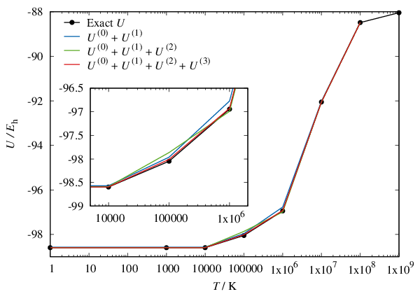
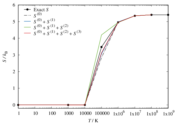
Figures 20 and 21 plot the perturbation approximations to and and their FCI values as a function of temperature. It can be seen that the perturbation approximations are so accurate that they are indiscernible from the FCI curves at both low and high temperatures. Only at mid-temperatures () are the differences noticeable. This is the same temperature domain where these thermodynamic functions exhibit strong temperature dependence and the perturbation series tend to diverge. Still, low-order perturbation theories seem to work well, correcting the vast majority of the discrepancies between the zeroth-order (Fermi–Dirac) theory and FCI in ( is not shown in Fig. 20 because it is far outside the graph). For , the first-order approximation overcorrects the errors in in this temperature domain, while the second- and third-order approximations roughly halve the errors. Given the divergence of the underlying perturbation series at these temperatures, the lower-order perturbation theories are promising.
VI.3 Canonical ensemble
| Recursion11 1 MBPT() recursions. The entries with fewer significant figures suffer from large round-off errors. | -variation22 2 Central seven-point formula with . See also Ref. Jha and Hirata 2020. | Recursion11 1 MBPT() recursions. The entries with fewer significant figures suffer from large round-off errors. | -variation22 2 Central seven-point formula with . See also Ref. Jha and Hirata 2020. | |
|---|---|---|---|---|
| 0 | ||||
| 1 | ||||
| 2 | ||||
| 3 | ||||
| 4 | ||||
| 5 | ||||
| 6 | ||||
| 7 | ||||
| 8 | ||||
| 9 | ||||
| 10 | ||||
| FCI33 3 Finite-temperature full configuration interaction. See also Ref. Kou and Hirata 2014. | ||||
| Recursion11 1 MBPT() recursions. | -variation22 2 Central seven-point formula with . See also Ref. Jha and Hirata 2020. | Recursion11 1 MBPT() recursions. | -variation22 2 Central seven-point formula with . See also Ref. Jha and Hirata 2020. | |
|---|---|---|---|---|
| 0 | ||||
| 1 | ||||
| 2 | ||||
| 3 | ||||
| 4 | ||||
| 5 | ||||
| 6 | ||||
| 7 | ||||
| 8 | ||||
| 9 | ||||
| 10 | ||||
| FCI33 3 Finite-temperature full configuration interaction. See also Ref. Kou and Hirata 2014. | ||||
| Recursion11 1 MBPT() recursions. | -variation22 2 Central seven-point formula with . See also Ref. Jha and Hirata 2020. | Recursion11 1 MBPT() recursions. | -variation22 2 Central seven-point formula with . See also Ref. Jha and Hirata 2020. | |
|---|---|---|---|---|
| 0 | ||||
| 1 | ||||
| 2 | ||||
| 3 | ||||
| 4 | ||||
| 5 | ||||
| 6 | ||||
| 7 | ||||
| 8 | ||||
| 9 | ||||
| 10 | ||||
| FCI33 3 Finite-temperature full configuration interaction. See also Ref. Kou and Hirata 2014. | ||||
Thermodynamic functions in the canonical ensemble have been calculated for the same system as Sec. VI.2. The results at , , and K are summarized in Tables 6, 7, and 8, respectively. Only the sum-over-states (recursion) formulas and -variation method are available for this ensemble.
Owing to the much fewer number of states involved in the canonical ensemble, the thermodynamic functions are less prone to divergence and the -variation method tends to be more accurate. At and K, the tenth-order perturbation theory agrees with FCI for five and ten decimal places, respectively, which attests to the convergence of the perturbation series to exactness at any temperature unless they diverge.
VII Conclusions
We have fully developed the finite-temperature MBPT that expands all thermodynamic functions in uniform perturbation series. Both grand canonical and canonical ensembles are considered, although only the former lends itself to more drastic mathematical simplifications, making it useful for condensed-matter applications. The Rayleigh–Schrödinger-like algebraic recursions have been obtained for both, yielding their sum-over-states analytical formulas of all thermodynamic functions at any arbitrary order.
For the grand canonical ensemble, the sum-over-states formulas have been transformed to sum-over-orbitals analytical formulas by the method of normal-ordered second quantization at finite temperature. The rules of Wick contractions and various operators in the normal-ordered form have been derived (as opposed to postulated) and how they are practically applied to integral and thermal-average evaluations has been illustrated. Feynman diagrammatic rules are then introduced as a straightforward graphical representation of Wick contractions as lines and of molecular integrals as vertexes. Nowhere in this formulation do we resort to time-dependent logicMatsubara 1955; Bloch and De Dominicis 1958; Kohn and Luttinger 1960; Luttinger and Ward 1960; Balian, Bloch, and De Dominicis 1961; Bloch 1965 or human intuitions to exhaustively enumerate all valid diagrams, which include the renormalization, anomalous, and anomalous renormalization diagrams.
Normal ordering regroups the Hamiltonian operator into the finite-temperature HF energy, finite-temperature Fock matrix elements times one-electron operators, and two-electron integrals times two-electron operators. This natural partitioning underscores the significance of the finite-temperature HF theory as the foundation of all converging finite-temperature electron-correlation theories. Its energy expression is identified with , which differs from either or at .
In the nondegenerate, zero-temperature MBPT, the renormalization terms cancel exactly the unlinked contribution of the equal magnitude in the parent term, ensuring the size-consistency of MBPT at any order, as proven by the linked-diagram theorem.Gell-Mann and Low 1951; Brueckner 1955; Goldstone 1957; Hugenholtz 1957; Frantz and Mills 1960; Manne 1977 In the finite-temperature MBPT, which sums over all possible states many of which are degenerate, the renormalization terms consist of both linked and unlinked contributions. The unlinked contribution cancels the same in the parent term, restoring the linkedness of the perturbation corrections at any order, while nonzero linked renormalization terms persist. They correspond to diagrams whose resolvent lines are displaced upwards in all possible ways so that there are two or more resolvents in between some pairs of adjacent vertexes and none in between others. These renormalization diagrams are distinguished from the well-known anomalous diagrams whose resolvent lines are deleted. They both are essential numerically, and had it not for them, the perturbation series would not converge at the finite-temperature FCI limit. It is unclear whether the conventional time-dependent, diagrammatic formulationMatsubara 1955; Bloch and De Dominicis 1958; Kohn and Luttinger 1960; Luttinger and Ward 1960; Balian, Bloch, and De Dominicis 1961; Bloch 1965 or density-matrix derivationSantra and Schirmer 2017 are aware of such diagrams.
We have proven the linked-diagram theorem of the finite-temperature MBPT. The theorem is based on the linked-diagram theorem at zero temperatureGell-Mann and Low 1951; Brueckner 1955; Goldstone 1957; Hugenholtz 1957; Frantz and Mills 1960; Manne 1977 and the systematic cancellation of unlinked anomalous diagrams.
We have derived reduced analytical formulas for the perturbation corrections to thermodynamic functions in the grand canonical ensemble up to the third order. We have also implemented general-order algorithms in both ensemble, and calculated the benchmark perturbation corrections up to the tenth order. At intermediate temperatures, where thermodynamic functions vary with temperature considerably, the perturbation series tend to diverge, but elsewhere they converge rapidly towards the finite-temperature FCI limits, establishing the correctness of the theory.
In a separate study,Hirata 2021 we showed that the finite-temperature MBPT at the first and second orders does not converge at the correct zero-temperature limit when the reference wave function is qualitatively different from the exact one, confirming Kohn and Luttinger.Kohn and Luttinger 1960 This originates from the nonanalyticity of the Boltzmann factor and is therefore expected to plague most any finite-temperature MBPT, e.g., the one in the canonical ensemble also.Jha and Hirata 2020 Nonconvergence should persist at third and all higher orders under the same condition.
This study and another reported in Ref. Hirata et al. 2017 have been conducted to lay a firm mathematical foundation of perturbation theories,Bartlett 1981; Hirata et al. 2014 which continue to be a workhorse for efficient, size-consistent,Hirata 2011; Hirata and Grabowski 2014 converging ab initio electronic structure calculationsWillow, Kim, and Hirata 2012; Willow, Kim, and Hirata 2013; Willow et al. 2013; Willow and Hirata 2014; Willow, Kim, and Hirata 2014b; Willow et al. 2014; Doran and Hirata 2016; Johnson et al. 2016; Johnson et al. 2018; Doran and Hirata 2019; Doran and Hirata 2020a; Doran and Hirata 2020b; Doran and Hirata 2021 for large complex molecules and solids.Grüneis et al. 2017 Unlike time-dependent, diagrammatic expositions,March, Young, and Sampanthar 1967; Thouless 1990; Mattuck 1992; Fetter and Walecka 2003 which are often incomplete and intractable, our derivations follow the transparent, linear, time-independent, algebraic logic, involving only elementary calculus and combinatorial identities. They justify the second-quantized and diagrammatic rules just as tools for expediency rather than rely on them as a graphical method of derivations that are often based on human intuitions detached from mathematics. Our derivation strategy can therefore be universally applied to any perturbation theory insofar as the exact limit is known, reliably leading to recursions, order-by-order analytical formulas, and general-order algorithms.
VIII Data Availability Statement
The data that supports the findings of this study are available within the article.
Acknowledgements.
The author thanks Professor Rodney J. Bartlett for teaching him the quantum-field-theoretical techniques used in this study. This work was supported by the Center for Scalable, Predictive methods for Excitation and Correlated phenomena (SPEC), which is funded by the U.S. Department of Energy, Office of Science, Office of Basic Energy Sciences, Chemical Sciences, Geosciences, and Biosciences Division, as a part of the Computational Chemical Sciences Program and also by the U.S. Department of Energy, Office of Science, Office of Basic Energy Sciences under Grant No. DE-SC0006028.Appendix A Recursions in the canonical ensemble
Thermodynamic functions in the canonical ensemble considered are the canonical partition function (), Helmholtz energy (), internal energy (), and entropy (), which are related to one another by
| (196) | |||||
| (197) | |||||
| (198) |
and
| (199) |
where the -summation goes over all spin states with a fixed total number () of electrons. The recursion for is given by
| (200) | |||||
where is defined differently from Eq. (12) only in this appendix as
| (201) |
The recursion for is inferred from Eq. (15) as
| (202) | |||||
Likewise, is defined recursively by
| (203) | |||||
which implies the recursion for .
These have been obtained by restricting the summations to -electron states and setting for all in the corresponding recursions for the grand canonical ensemble.
Appendix B A proof of equivalence of Eqs. (13) and (14)
Generally, we prove the equivalence of two recursions,
| (204) | |||||
and
| (205) | |||||
Equations (13) and (14) are a special case of these in which and . We can rewrite the second equation as
| (206) | |||||
Substituting this into the right-hand side of Eq. (204), we can convert it into a form expressed entirely in terms of as
| (207) | |||||
We shall show that and ().
By inspection, we find , , and . In general, the coefficient multiplying () is given as
| (208) |
where is the Stirling number of the second kind (the number of ways objects are partitioned into nonempty sets).Kao and Zetterberg 1957 It is defined as
| (209) |
where the summation goes over all natural numbers that satisfy . There is an identity involving the Stirling number, which reads
| (210) |
which implies (), proving the equivalence.
The identity (210) can in turn be proven by induction using the recursion:
| (211) |
Equation (210) is true for . If it is true for , it also holds true for and therefore for any because
| (212) |
where we used .
Finally, the recursion for the Stirling number [Eq. (211)] can be justified as follows: The left-hand side counts the number of ways objects are partitioned into nonempty sets. The first term in the right-hand side is the number of ways in which the th object is absorbed into one of the existing nonempty sets of the first objects. The second term is the number of ways in which the th object forms a new (th) set containing only it and the first objects are partitioned into nonempty sets.
Appendix C Normal-ordered second quantization at finite temperature
In this appendix, we fully develop the normal-ordered second quantization at finite temperatureMarch, Young, and Sampanthar 1967; Sanyal et al. 1993 within the time-independent framework in a transparent and pedagogical manner. It serves as a basis of the diagrammatic derivation and the linked-diagram theorem. The reader is referred to Shavitt and Bartlett Shavitt and Bartlett 2009 for normal-ordered second quantization at zero temperature and to March, Young, and SampantharMarch, Young, and Sampanthar 1967 for an abridged exposition of its finite-temperature counterpart. The following expounds on the latter with enough details to be actually used in deriving the second-order formulas in Sec. III.
C.1 Normal ordering at finite temperature
A product of creation () and annihilation () operators in the normal order (denoted by ) is defined [cf. Eq. (9.3.2) of Ref. March, Young, and Sampanthar 1967] as
| (215) | |||||
| (216) |
where and are the Fermi–Dirac distribution functions given by Eqs. (102) and (103). When ,
| (217) | |||||
| (218) |
A normal-ordered product of two creation operators or of two annihilation operators is also the same as the original order.
In analogy to the zero-temperature case, the normal ordering at finite temperature is designed so that the thermal average of a normal-ordered product is always zero. Using Einstein’s convention of implied summations of repeated spinorbital indexes, we confirm
| (219) | |||||
where we used the Boltzmann sum identities I and V of Ref. Hirata and Jha 2020 in the penultimate equality.
Next, we define a Wick contraction (denoted by a staple symbol) as the difference between the operator product and its normal-ordered counterpart.
| (220) | |||||
| (221) |
where we used the anticommutation rules of fermion creation and annihilation operators. When ,
| (222) | |||||
| (223) |
A Wick contraction of two creation or of two annihilation operators is also zero.
The concept of the normal ordering can be generalized to any even number of operators. For instance, a product of four operators in the normal order is defined as (),
| (224) | |||||
| (226) | |||||
When or ,
| (227) |
The thermal average of a normal-ordered product of any number of operators is also always zero by construction. This can be verified for the above product as follows:
| (228) |
where Boltzmann sum identities III, V, and IX of Ref. Hirata and Jha 2020 were used.
For a product of more than two operators, there are two types of contractions: partial and full contractions. Together, they are defined as
where in the right-hand side gathers the uncontracted operators (kept in the original order), and is the number of permutations necessary to reorder the whole operator sequence from the left- to right-hand side. If there are no operators left in , it is a full contraction; otherwise it is a partial contraction. A full contraction is a real number, while a partial contraction is a normal-ordered operator multiplied by a real number. The parity of a full contraction is () for an even (odd) number of intersections of the staple symbols of Wick contractions.Shavitt and Bartlett 2009
C.2 Wick’s theorem at finite temperature
Wick’s theorem states that a product of operators is the sum of its normal-ordered product and all of its partial and full contractions.Shavitt and Bartlett 2009 This holds true at zero and nonzero temperatures. For a product of two operators, the theorem is just a restatement of the definitions of Wick contractions:
| (230) | |||||
| (231) |
For a product of four operators, the theorem asserts
| (232) | |||||
We can verify this for the following simpler, but nontrivial case by inspection:
| (237) | |||||
| (238) |
When or , Eq. (227) embodies the theorem. In general situations, the theorem can be proven by induction. See Ref. Shavitt and Bartlett 2009 for an outline of the proof for the zero-temperature case.
Since the thermal average of any normal-ordered product of operators vanishes, a nonzero thermal average arises solely from full contractions, e.g.,
However, more frequently, we need to evaluate the thermal average of a product of two or more normal-ordered products. We show that such a product is the sum of concatenated normal-ordered product plus all of its partial and full contractions excluding internal contractions. An internal contraction is the one that involves at least one contraction within an original normal-ordered product. The following is an illustration of this rule:
Internal contractions in this example are the ones that contract with and/or with , which are therefore excluded from the right-hand side. This rule can be justified by comparing Eq. (232) with
The last three terms are internal contractions, which cancel out the same in Eq. (232) when equated with the above. Therefore, the thermal average of a product of normal-ordered products comes solely from its full contractions excluding internal contractions, e.g.,
| (242) | |||||
C.3 Hamiltonian and number operators
Let us express the number operator in the normal-ordered second quantization at finite temperature.
| (243) | |||||
where we used the zeroth-order electroneutrality condition [Eq. (104)] in the last equality. Taking the thermal average of the above equation, we immediately find .
The Hamiltonian operator in second quantization is written asShavitt and Bartlett 2009; Szabo and Ostlund 1982
| (244) |
where is the nucleus-nucleus repulsion energy, is the integral of the one-electron part of the Hamiltonian operator, and is the antisymmetrized two-electron integral. This can be finite-temperature normal ordered as
where and are the finite-temperature Hartree–Fock energy and Fock matrix element,Mermin 1963 defined by
| (246) | |||||
| (247) |
Therefore, is identified as the following sum,
| (248) |
where the thermal averages of the zeroth- and first-order energy correctionsHirata and Jha 2019; Hirata and Jha 2020 are given by
| (249) | |||||
| (250) |
with being the difference between the finite-temperature Fock and diagonal zero-temperature Fock matrix elements,
| (251) |
Equation (248) mirrors the well-known identitySzabo and Ostlund 1982 in the zero-temperature case, , but it does not agree with either or at . They are instead related to one another byHirata and Jha 2019; Hirata and Jha 2020
| (252) | |||||
| (253) | |||||
We employ the Møller–Plesset partitioningMøller and Plesset 1934 of the Hamiltonian. The zeroth-order Hamiltonian and perturbation operators are then written in the normal-ordered form as
| (254) | |||||
C.4 Projector and resolvent operator
In order to understand the second-quantization rule for the resolvent operator, let us first examine the effect of inserting the resolution-of-the-identity in Eq. (242). Using Einstein’s implied summation of repeated spinorbital and state indexes, we can rewrite Eq. (242) as
| (256) |
where runs over all determinants, and hence . In the second equality, we wrote . For the last equality to hold, we should regard a chain of contractions, -- or --, as a single contraction evaluated as or , respectively, rather than view each as three consecutive contractions evaluated as or , which is erroneous.
Then, the rule for evaluating thermal averages involving a resolvent operator is essentially the same. To explain the rule by a similar example, we may consider
| (257) |
where stands for a determinant outside the degenerate subspace of , which explains why the summations over and must be restricted (“”) to nonzero denominators. In other words, acts as an outer projector.
Let us define inner projector , where runs over only those determinants that are degenerate with .
| (258) |
where the summations over and are now restricted (“”) to the cases whose fictitious denominator () is zero.
References
- Kurashige and Yanai (2009) Y. Kurashige and T. Yanai, J. Chem. Phys. 130, 234114 (2009).
- Zgid and Chan (2011) D. Zgid and G. K.-L. Chan, J. Chem. Phys. 134, 094115 (2011).
- Booth et al. (2011) G. H. Booth, D. Cleland, A. J. W. Thom, and A. Alavi, J. Chem. Phys. 135, 084104 (2011).
- Ellis, Martin, and Scuseria (2013) J. K. Ellis, R. L. Martin, and G. E. Scuseria, J. Chem. Theory Comput. 9, 2857 (2013).
- Bytautas, Scuseria, and Ruedenberg (2015) L. Bytautas, G. E. Scuseria, and K. Ruedenberg, J. Chem. Phys. 143, 094105 (2015).
- Ohtsuka and Ten-no (2015) Y. Ohtsuka and S. Ten-no, J. Chem. Phys. 143, 144116 (2015).
- Chan et al. (2016) G. K.-L. Chan, A. Keselman, N. Nakatani, Z. D. Li, and S. R. White, J. Chem. Phys. 145, 014102 (2016).
- Holmes, Tubman, and Umrigar (2016) A. A. Holmes, N. M. Tubman, and C. J. Umrigar, J. Chem. Theory Comput. 12, 3674 (2016).
- He et al. (2019) Y. Y. He, M. P. Qin, H. Shi, Z. Y. Lu, and S. W. Zhang, Phys. Rev. B 99, 045108 (2019).
- Baiardi and Reiher (2020) A. Baiardi and M. Reiher, J. Chem. Phys. 152, 040903 (2020).
- Stair and Evangelista (2020) N. H. Stair and F. A. Evangelista, J. Chem. Phys. 153, 104108 (2020).
- Cui, Zhu, and Chan (2020) Z. H. Cui, T. Y. Zhu, and G. K.-L. Chan, J. Chem. Theory Comput. 16, 119 (2020).
- Deustua, Shen, and Piecuch (2021) J. E. Deustua, J. Shen, and P. Piecuch, J. Chem. Phys. 154, 124103 (2021).
- Motta et al. (2017) M. Motta, D. M. Ceperley, G. K.-L. Chan, J. A. Gomez, E. Gull, S. Guo, C. A. Jiménez-Hoyos, T. N. Lan, J. Li, F. J. Ma, A. J. Millis, N. V. Prokof’ev, U. Ray, G. E. Scuseria, S. Sorella, E. M. Stoudenmire, Q. M. Sun, I. S. Tupitsyn, S. R. White, D. Zgid, and S. W. Zhang, Phys. Rev. X 7, 031059 (2017).
- Williams et al. (2020) K. T. Williams, Y. Yao, J. Li, L. Chen, H. Shi, M. Motta, C. Y. Niu, U. Ray, S. Guo, R. J. Anderson, J. H. Li, L. N. Tran, C. N. Yeh, B. Mussard, S. Sharma, F. Bruneval, M. van Schilfgaarde, G. H. Booth, G. K.-L. Chan, S. W. Zhang, E. Gull, D. Zgid, A. Millis, C. J. Umrigar, and L. K. Wagner, Phys. Rev. X 10, 011041 (2020).
- Lee, Nagaosa, and Wen (2006) P. A. Lee, N. Nagaosa, and X. G. Wen, Rev. Mod. Phys. 78, 17 (2006).
- Phillips, Choy, and Leigh (2009) P. Phillips, T. P. Choy, and R. G. Leigh, Rep. Prog. Phys. 72, 036501 (2009).
- Su, Schrieffer, and Heeger (1979) W. P. Su, J. R. Schrieffer, and A. J. Heeger, Phys. Rev. Lett. 42, 1698 (1979).
- Heeger et al. (1988) A. J. Heeger, S. Kivelson, J. R. Schrieffer, and W. P. Su, Rev. Mod. Phys. 60, 781 (1988).
- Anderson (1990) P. W. Anderson, Phys. Rev. Lett. 64, 1839 (1990).
- Kittel (1987) C. Kittel, Quantum Theory of Solids, 2nd ed. (Wiley, Dehli, 1987).
- Tinkham (1996) M. Tinkham, Introduction to Superconductivity, 2nd ed. (Dover, New York, 1996).
- Kresin, Morawitz, and Wolf (2014) V. Z. Kresin, H. Morawitz, and S. A. Wolf, Superconducting State: Mechanisms and Properties (Oxford University Press, Oxford, 2014).
- Overhauser (1960) A. W. Overhauser, Phys. Rev. Lett. 4, 462 (1960).
- Overhauser (1962) A. W. Overhauser, Phys. Rev. 128, 1437 (1962).
- Čížek and Paldus (1967) J. Čížek and J. Paldus, J. Chem. Phys. 47, 3976 (1967).
- Yamada and Hirata (2015) T. Yamada and S. Hirata, J. Chem. Phys. 143, 114112 (2015).
- Sanyal et al. (1993) G. Sanyal, S. H. Mandal, S. Guha, and D. Mukherjee, Phys. Rev. E 48, 3373 (1993).
- Mandal, Ghosh, and Mukherjee (2001) S. H. Mandal, R. Ghosh, and D. Mukherjee, Chem. Phys. Lett. 335, 281 (2001).
- Mandal et al. (2002) S. H. Mandal, R. Ghosh, G. Sanyal, and D. Mukherjee, in Recent Progress in Many-Body Theories, edited by R. Bishop, T. Brandes, K. A. Gernoth, N. R. Walet, and Y. Xian (World Scientific, Singapore, 2002) pp. 383–392.
- Malone et al. (2016) F. D. Malone, N. S. Blunt, E. W. Brown, D. K. K. Lee, J. S. Spencer, W. M. C. Foulkes, and J. J. Shepherd, Phys. Rev. Lett. 117, 115701 (2016).
- Rusakov and Zgid (2016) A. A. Rusakov and D. Zgid, J. Chem. Phys. 144, 054106 (2016).
- Welden, Rusakov, and Zgid (2016) A. R. Welden, A. A. Rusakov, and D. Zgid, J. Chem. Phys. 145, 204106 (2016).
- White and Chan (2018) A. F. White and G. K.-L. Chan, J. Chem. Theory Comput. 14, 5690 (2018).
- Harsha, Henderson, and Scuseria (2019a) G. Harsha, T. M. Henderson, and G. E. Scuseria, J. Chem. Phys. 150, 154109 (2019a).
- Harsha, Henderson, and Scuseria (2019b) G. Harsha, T. M. Henderson, and G. E. Scuseria, J. Chem. Theory Comput. 15, 6127 (2019b).
- Liu et al. (2020) Y. Liu, T. Shen, H. Zhang, and B. Rubenstein, J. Chem. Theory Comput. 16, 4298 (2020).
- Harsha, Henderson, and Scuseria (2020) G. Harsha, T. M. Henderson, and G. E. Scuseria, J. Chem. Phys. 153, 124115 (2020).
- Barghathi, Yu, and Del Maestro (2020) H. Barghathi, J. Yu, and A. Del Maestro, Phys. Rev. Research 2, 043206 (2020).
- Sun et al. (2020) C. Sun, U. Ray, Z. H. Cui, M. Stoudenmire, M. Ferrero, and G. K.-L. Chan, Phys. Rev. B 101, 075131 (2020).
- Lee, Morales, and Malone (2021) J. Lee, M. A. Morales, and F. D. Malone, J. Chem. Phys. 154, 064109 (2021).
- March, Young, and Sampanthar (1967) N. H. March, W. H. Young, and S. Sampanthar, The Many-Body Problem in Quantum Mechanics (Cambridge University Press, Cambridge, 1967).
- Thouless (1990) D. J. Thouless, The Quantum Mechanics of Many-Body Systems, 2nd ed. (Dover, New York, 1990).
- Mattuck (1992) R. D. Mattuck, A Guide to Feynman Diagrams in the Many-Body Problem (Dover, New York, 1992).
- Fetter and Walecka (2003) A. L. Fetter and J. D. Walecka, Quantum Theory of Many-Particle Systems (Dover, New York, 2003).
- Matsubara (1955) T. Matsubara, Prog. Theor. Phys. 14, 351 (1955).
- Bloch and De Dominicis (1958) C. Bloch and C. De Dominicis, Nucl. Phys. 7, 459 (1958).
- Kohn and Luttinger (1960) W. Kohn and J. M. Luttinger, Phys. Rev. 118, 41 (1960).
- Luttinger and Ward (1960) J. M. Luttinger and J. C. Ward, Phys. Rev. 118, 1417 (1960).
- Balian, Bloch, and De Dominicis (1961) R. Balian, C. Bloch, and C. De Dominicis, Nucl. Phys. 25, 529 (1961).
- Bloch (1965) C. Bloch, in Studies in Statistical Mechanics, edited by J. De Boer and G. E. Uhlenbeck (North Holland, Amsterdam, 1965) pp. 3–211.
- Santra and Schirmer (2017) R. Santra and J. Schirmer, Chem. Phys. 482, 355 (2017).
- Jha and Hirata (2019) P. K. Jha and S. Hirata, Annu. Rep. Comput. Chem. 15, 3 (2019).
- Hirata and Jha (2019) S. Hirata and P. K. Jha, Annu. Rep. Comput. Chem. 15, 17 (2019).
- Hirata and Jha (2020) S. Hirata and P. K. Jha, J. Chem. Phys. 153, 014103 (2020).
- Hirata (2021) S. Hirata, Phys. Rev. A 103, 012223 (2021).
- Kou and Hirata (2014) Z. Kou and S. Hirata, Theor. Chem. Acc. 133, 1487 (2014).
- Mermin (1963) N. D. Mermin, Ann. Phys. 21, 99 (1963).
- Hirata et al. (2017) S. Hirata, A. E. Doran, P. J. Knowles, and J. V. Ortiz, J. Chem. Phys. 147, 044108 (2017).
- Pain (2011) J. C. Pain, J. Phys. B. At. Mol. Opt. 44, 145001 (2011).
- Hirschfelder and Certain (1974) J. O. Hirschfelder and P. R. Certain, J. Chem. Phys. 60, 1118 (1974).
- Jha and Hirata (2020) P. K. Jha and S. Hirata, Phys. Rev. E 101, 022106 (2020).
- Shavitt and Bartlett (2009) I. Shavitt and R. J. Bartlett, Many-Body Methods in Chemistry and Physics (Cambridge University Press, Cambridge, 2009).
- Hirata (2011) S. Hirata, Theor. Chem. Acc. 129, 727 (2011).
- Gell-Mann and Low (1951) M. Gell-Mann and F. Low, Phys. Rev. 84, 350 (1951).
- Brueckner (1955) K. A. Brueckner, Phys. Rev. 100, 36 (1955).
- Goldstone (1957) J. Goldstone, Proc. Roy. Soc. A (London) 239, 267 (1957).
- Hugenholtz (1957) N. M. Hugenholtz, Physica 23, 481 (1957).
- Frantz and Mills (1960) L. M. Frantz and R. L. Mills, Nucl. Phys. 15, 16 (1960).
- Manne (1977) R. Manne, Int. J. Quantum Chem. Symp. 11, 175 (1977).
- Harris, Monkhorst, and Freeman (1992) F. E. Harris, H. J. Monkhorst, and D. L. Freeman, Algebraic and Diagrammatic Methods in Many-Fermion Theory (Oxford University Press, Oxford, 1992).
- Møller and Plesset (1934) C. Møller and M. S. Plesset, Phys. Rev. 46, 618 (1934).
- Klein (1974) D. J. Klein, J. Chem. Phys. 61, 786 (1974).
- Szabo and Ostlund (1982) A. Szabo and N. S. Ostlund, Modern Quantum Chemistry (MacMillan, New York, 1982).
- Hirata et al. (2015) S. Hirata, M. R. Hermes, J. Simons, and J. V. Ortiz, J. Chem. Theory Comput. 11, 1595 (2015).
- Hirata (2003) S. Hirata, J. Phys. Chem. A 107, 9887 (2003).
- Bartlett and Noga (1988) R. J. Bartlett and J. Noga, Chem. Phys. Lett. 150, 29 (1988).
- Knowles et al. (1985) P. J. Knowles, K. Somasundram, N. C. Handy, and K. Hirao, Chem. Phys. Lett. 113, 8 (1985).
- Hirata and Bartlett (2000) S. Hirata and R. J. Bartlett, Chem. Phys. Lett. 321, 216 (2000).
- Kállay and Surján (2000) M. Kállay and P. R. Surján, J. Chem. Phys. 113, 1359 (2000).
- Olsen (2000) J. Olsen, J. Chem. Phys. 113, 7140 (2000).
- Hirata, Nooijen, and Bartlett (2000a) S. Hirata, M. Nooijen, and R. J. Bartlett, Chem. Phys. Lett. 326, 255 (2000a).
- Hirata, Nooijen, and Bartlett (2000b) S. Hirata, M. Nooijen, and R. J. Bartlett, Chem. Phys. Lett. 328, 459 (2000b).
- Shimazaki and Hirata (2009) T. Shimazaki and S. Hirata, Int. J. Quantum Chem. 109, 2953 (2009).
- Hirata and Shimazaki (2009) S. Hirata and T. Shimazaki, Phys. Rev. B 80, 085118 (2009).
- Ohnishi and Hirata (2010) Y.-y. Ohnishi and S. Hirata, J. Chem. Phys. 133, 034106 (2010).
- Ohnishi and Hirata (2011) Y.-y. Ohnishi and S. Hirata, J. Chem. Phys. 135, 094108 (2011).
- Willow, Kim, and Hirata (2014a) S. Y. Willow, K. S. Kim, and S. Hirata, Phys. Rev. B 90, 201110(R) (2014a).
- He, Ryu, and Hirata (2014) X. He, S. Ryu, and S. Hirata, J. Chem. Phys. 140, 024702 (2014).
- Hermes and Hirata (2015) M. R. Hermes and S. Hirata, J. Chem. Phys. 143, 102818 (2015).
- Saha (1920) M. N. Saha, Philos. Mag. 40, 472 (1920).
- Saha (1921) M. N. Saha, Proc. Roy. Soc. (London) A 99, 135 (1921).
- Brändas and Bartlett (1971) E. J. Brändas and R. J. Bartlett, Chem. Phys. Lett. 8, 153 (1971).
- Bender and Orszag (1978) C. M. Bender and S. A. Orszag, Advanced Mathematical Methods for Scientist and Engineers I: Asymptotic Methods and Perturbation Theory (McGraw-Hill, New York, 1978).
- Laidig, Fitzgerald, and Bartlett (1985) W. D. Laidig, G. Fitzgerald, and R. J. Bartlett, Chem. Phys. Lett. 113, 151 (1985).
- Olsen et al. (1996) J. Olsen, O. Christiansen, H. Koch, and P. Jørgensen, J. Chem. Phys. 105, 5082 (1996).
- Bartlett (1981) R. J. Bartlett, Annu. Rev. Phys. Chem. 32, 359 (1981).
- Hirata et al. (2014) S. Hirata, X. He, M. R. Hermes, and S. Y. Willow, J. Phys. Chem. A 118, 655 (2014).
- Hirata and Grabowski (2014) S. Hirata and I. Grabowski, Theor. Chem. Acc. 133, 1440 (2014).
- Willow, Kim, and Hirata (2012) S. Y. Willow, K. S. Kim, and S. Hirata, J. Chem. Phys. 137, 204122 (2012).
- Willow, Kim, and Hirata (2013) S. Y. Willow, K. S. Kim, and S. Hirata, J. Chem. Phys. 138, 164111 (2013).
- Willow et al. (2013) S. Y. Willow, M. R. Hermes, K. S. Kim, and S. Hirata, J. Chem. Theory Comput. 9, 4396 (2013).
- Willow and Hirata (2014) S. Y. Willow and S. Hirata, J. Chem. Phys. 140, 024111 (2014).
- Willow, Kim, and Hirata (2014b) S. Y. Willow, K. S. Kim, and S. Hirata, Phys. Rev. B 90, 201110 (2014b).
- Willow et al. (2014) S. Y. Willow, J. Zhang, E. F. Valeev, and S. Hirata, J. Chem. Phys. 140, 031101 (2014).
- Doran and Hirata (2016) A. E. Doran and S. Hirata, J. Chem. Theory Comput. 12, 4821 (2016).
- Johnson et al. (2016) C. M. Johnson, A. E. Doran, J. Zhang, E. F. Valeev, and S. Hirata, J. Chem. Phys. 145, 154115 (2016).
- Johnson et al. (2018) C. M. Johnson, A. E. Doran, S. L. Ten-no, and S. Hirata, J. Chem. Phys. 149, 174112 (2018).
- Doran and Hirata (2019) A. E. Doran and S. Hirata, J. Chem. Theory Comput. 15, 6097 (2019).
- Doran and Hirata (2020a) A. E. Doran and S. Hirata, J. Chem. Phys. 153, 094108 (2020a).
- Doran and Hirata (2020b) A. E. Doran and S. Hirata, J. Chem. Phys. 153, 104112 (2020b).
- Doran and Hirata (2021) A. E. Doran and S. Hirata, J. Chem. Phys. 154, 134114 (2021).
- Grüneis et al. (2017) A. Grüneis, S. Hirata, Y.-y. Ohnishi, and S. Ten-no, J. Chem. Phys. 146, 080901 (2017).
- Kao and Zetterberg (1957) R. C. Kao and L. H. Zetterberg, Amer. Math. Monthly 64, 96 (1957).