Analytical and numerical study of the hidden boundary of practical stability:
complex versus real Lorenz systems
Abstract
This work presents the continuation of the recent article ”The Lorenz system: hidden boundary of practical stability and the Lyapunov dimension” KuznetsovMKKL-2020, published in the Nonlinear Dynamics journal. In this work, in comparison with the results for classical real-valued Lorenz system (henceforward – Lorenz system), the problem of analytical and numerical identification of the boundary of global stability for the complex-valued Lorenz system (henceforward – complex Lorenz system) is studied. As in the case of the Lorenz system, to estimate the inner boundary of global stability the possibility of using the mathematical apparatus of Lyapunov functions (namely, the Barbashin-Krasovskii and LaSalle theorems) is demonstrated. For additional analysis of homoclinic bifurcations in complex Lorenz system a special analytical approach by Vladimirov is utilized. To outline the outer boundary of global stability and identify the so-called hidden boundary of global stability, possible birth of hidden attractors and transient chaotic sets is analyzed.
Keywords:
chaos, Lorenz system, complex Lorenz system, boundary of global stability, hidden attractors, transient chaosI Introduction
In the study of the dynamics of applied systems, an important role is played by the property of global stability11 1 We use the term “global stability” for simplicity of further presentation, while in the literature there are used different notions, e.g. “globally asymptotically stable” (Vidyasagar-1978, p. 137), (HaddadC-2011, p. 144), “gradient-like” (LeonovRS-1992, p. 2), (YakubovichLG-2004, p. 56), “quasi-gradient-like” (LeonovRS-1992, p. 2), (YakubovichLG-2004, p. 56) and others, reflecting the features of the stationary set and the convergence of trajectories to it. , when there are no oscillations in the system, and all trajectories are attracted to a stationary set. In some cases, the global stability property can be established analytically (e.g. by Lyapunov-type, either frequency-domain methods, see BarbashinK-1952; Lasalle-1960; LeonovPS-1996; KuznetsovLYYKKRA-2020-ECC), and the global stability boundary can be constructed in the parameter space. Crossing this analytical boundary can lead to the following scenarios. After crossing the analytical border of global stability, the system can still exhibits practical22 2 Let us remark here a different notion of practical stability, suggested and developed in LaSalleL-1961; LakshmikanthamLM-1990. According to this notion, a unique equilibrium of a perturbed system is practically stable, if for all bounded perturbations and all initial points from a vicinity of equilibrium, corresponding trajectories stay inside a larger vicinity for all moments of time; at the same time, the equilibrium can be Lyapunov unstable. global stability KuznetsovMKKL-2020, i.e. almost all trajectories are attracted to a stationary set, however, in this case a countable number of orbits may appear, which nevertheless are not realized in practice and in standard numerical experiments (e.g., unstable periodic or homoclinic orbits AfraimovicBSh-1977; AuerbachCEGP-1987; Cvitanovic-1991; ShilnikovTCh-2001; Leonov-2013-IJBC; LeonovKM-2015-EPJST; LeonovMKM-2020-IJBC). On the other hand, crossing the analytical boundary of global stability can lead to the loss of stability of the stationary set. Then, if the system is dissipative in the sense Levinson (Levinson-1944, see also LeonovKM-2015-EPJST), but all stationary points are unstable, then inside the absorbing set a self-excited nontrivial attractor can be observed and easily localized. Finally, after crossing the boundary of global stability, the stationary set can remain locally stable (or partially locally stable), but at the same time hidden oscillations (periodic or chaotic) LeonovKV-2011-PLA; LeonovK-2013-IJBC; LeonovKM-2015-EPJST; Kuznetsov-2016; Kuznetsov-2020-TiSU may appear in the phase space, which basins of attraction do not intersect with arbitrarily small open vicinities of equilibria. This part of border of global stability, accordingly, can be also called ”hidden” Kuznetsov-2020-TiSU; KuznetsovMKKL-2020.
This work is the continuation of the recent article ”The Lorenz system: hidden boundary of practical stability and the Lyapunov dimension” KuznetsovMKKL-2020, where the analytical and numerical analysis of the boundary of global stability was performed for the classical Lorenz system Lorenz-1963:
| (1) |
where parameters , , . Here in the introduction, we briefly outline these results to compare them further with the results for the complex Lorenz system.
- 1)
Dissipativity. The Lorenz system (1) is dissipative in the sense of Levinson, since it has the absorbing set LeonovB-1992
(2) This implies that all solutions of (1) exist for and, thus, system (1) generates a dynamical system. For , the stationary set of system (1) consists of a unique stable equilibrium ; for a pair of symmetric equilibria is added to the stationary set, and turns into a saddle.
- 2)
Inner estimation of global stability. For the Lorenz system (1), combining several approaches based on the construction of Lyapunov functions BarbashinK-1952; Lasalle-1960; Leonov-2018-UMZh-rus it is possible to prove the following criterion for the absence of self-excited and hidden oscillations (see Figs. 1a, 1b).
Theorem 1.
Beyond the estimate (3) in Theorem 1, the analysis of global stability and the birth of nontrivial attractors can be performed numerically. It is further known that the separatrix of saddle can form a homoclinic loop from which unstable cycles can arise and violate the global stability (however, a set of measure zero does not affect the global attraction on a stationary set from a practical point of view). Using the Fishing principle Leonov-2013-IJBC; LeonovKM-2015-EPJST; LeonovMKM-2020-IJBC for the Lorenz system (1) it is possible to prove the following:
Theorem 2.
For and fixed, there exists corresponding to the homoclinic orbit of the saddle equilibrium if and only if .
For instance, for the classical values of parameters , of system (1) it is possible to find numerically the approximate value of such homoclinic bifurcation , when two symmetric homoclinic orbits forming a homoclinic butterfly appear (see Fig. 1c). Further increase of the parameter leads to the birth of two saddle periodic orbits from each homoclinic orbit ShilnikovTCh-2001.
(a) (b) (c) Figure 1: Dynamics of the Lorenz system (1) with fixed parameters , , when parameter varying according to the inner estimation of global stability. - 3)
Outer estimation of global stability. For systems with a global absorbing set and an unstable stationary set, the existence of self-excited attractors is obvious. From a computational perspective this allows one to use a standard computational procedure, in which after a transient process, a trajectory, starting from a point of unstable manifold in a neighborhood of equilibrium, reaches a state of oscillation, thus one can easily identify it.
System (1) possesses the absorbing set (see Eq. (2)) and for , all equilibria are unstable. Thus, in this case, system (1) has a nontrivial self-excited attractor: if we consider classical values of parameters , , then for , e.g. for , it is possible to observe the self-excited chaotic attractor with respect to all three equilibria , (see Fig. 2c).

(a) , hidden transient chaotic set 
(b) , self-excited attractor w.r.t 
(c) , self-excited attractor w.r.t , Figure 2: Dynamics of the Lorenz system (1) with fixed parameters , , when parameter varying according to the outer estimation of global stability. - 4)
Boundary of practical global stability. The presence of an absorbing set implies the existence of a globally attractor , which contains all local self-excited and hidden attractors, and stationary set. Thus, inside the set it is possible to study numerically the presence of nontrivial self-excited and hidden attractors for parameters , , not satisfying conditions (3) of global stability, i.e. by fixing and , and by decreasing from . For , , this gives us the following region , where , .
A nontrivial self-exited attractor can be observed numerically for (see e.g. Sparrow-1982). In this case of nontrivial multistability, system (1) possesses a local chaotic attractor which is self-excited with respect to equilibrium and co-exists with the trivial attractors (see Fig. 2b).
- 5)
Hidden attractor or transient set? For the Lorenz system (1) it is still an open question (Kuznetsov-2016, p. 14), whether for some parameters there exists a hidden chaotic attractor, i.e. whether it is possible by changing parameters to disconnect the basin of attraction from equilibria , (e.g. for the parameters , : if , then attractor is connected with , ; if , then attractor is connected with only ). The current results on the existence of the hidden attractors in the Lorenz system are the following: recently reported hidden attractors in the Lorenz system with and locally stable equilibria turn out to be a transient chaotic set (a set in the phase space, which can persist for a long time, but after all collapses), but not a sustained hidden chaotic attractor YuanYW-2017-HA; MunmuangsaenS-2018-HA.
In a numerical computation of a trajectory over a finite-time interval it is difficult to distinguish a sustained chaos from a transient chaos GrebogiOY-1983; LaiT-2011, thus it is reasonable to give a similar classification for transient chaotic sets DancaK-2017-CSF; ChenKLM-2017-IJBC: transient chaotic set is a hidden one if it does not involve and attract trajectories from a small neighborhood of equilibria; otherwise, it is self-excited.
For the Lorenz system (1) with parameters , fixed, near the point it is possible to observe a long living transient chaotic set, which is hidden since it’s basin of attraction does not intersect with the small vicinities of equilibrium (see Fig. 2a).
In our experiments, consider system (1) with parameters , , . Using MATLAB’s standard procedure ode45 with default parameters (relative tolerance , absolute tolerance ) for trajectory of system (1) with initial point a transient chaotic behavior is observed on the time interval , for initial point — on the time interval , for initial point — on the time interval , and for initial point a transient chaotic behavior continues over a time interval of more than . Remark that, if we consider the same initial points, but use MATLAB’s procedure ode45 with relative tolerance , for all these initial points the chaotic transient behavior will last over a time interval of more than , and corresponding transient chaotic sets won’t collapse.
II The complex Lorenz system
The classical Lorenz system (1) has gained and still attracts much attention of scientists33 3 The original celebrated work by Lorenz Lorenz-1963 has gained more than 24000 cites according to Google Scholar. , however, it is a rather simple mathematical model of the fluid dynamics problem, which E. Lorenz has initially investigated. A more complicated model of many real-world physical problems, such as two-layer baroclinic instability with weak viscosity and beta-effect GibbonM-1982; FowlerGM-1982; FowlerGM-1983 and detuned laser optics Ning-1990; NeimarkL-1992, is described by the following complex Lorenz system:
| (4) |
where , are complex variables, is real, and denotes complex conjugation operator. Parameters , are real, and are complex with . Note that since the transformation changes only the sign of in (4), this parameter may be chosen positive RauhHA-1996.
System (4) is also dissipative in the sense of Levinson, and the bounded convex absorbing set could be constructed according to the following theorem LeonovR-1987.
Theorem 3.
Let for there exist , , such that
| (5) |
Define , and the following function :
Then for any solution of (4) and any with , the following inequalities hold for all :
| (6) |
and
| (7) |
Thus, if condition (5) holds, then the solutions of system (4) exist for and, thus, system (4) generates a dynamical system and possesses a global attractor Chueshov-2002 containing a set of all equilibria.
It is also useful to consider the following equivalent form of system (4) in terms of real variables and real parameters (see, e.g. RauhHA-1996):
| (8) |
For
| (9) |
system (8) has a unique equilibrium . For
| (10) |
system (8) has a stationary set containing and a whole circle of equilibria given by the expression:
These equilibria could be parameterized as follows:
where and . In literature, relation is often called the ”laser case”, since in this case system (4) describe the dynamics of some lasers, e.g. a detuned laser Ning-1990; RauhHA-1996.
Let us outline the following statements about local stability of the stationary set of system (8) (see e.g. FowlerGM-1982).
Lemma 1.
The equilibrium of system (8) is stable if and only if the following condition hold:
Lemma 2.
The equilibria of system (8) are stable44 4 One could easily check that the eigenvalues of the Jacobi matrix at all equilibria are the same for any . if and only if one of the following conditions hold:
where
and , , .
III Inner estimation: the global stability and trivial attractors
Constructing complex-valued Lyapunov functions, by analogy with Theorem 1, it is possible to derive the following criterion for the absence of self-excited and hidden oscillations in the complex Lorenz system (4).
Theorem 4.
Proof.
We consider the following cases:
Case 1. For , one can check that conditions (9) are satisfied and in this case is the only equilibria of system (4). So, the absence of self-excited oscillations follows from the Routh-Hurwitz criterion on local stability for the equilibrium . The absence of hidden oscillations can be obtained by Barbashin-Krasovskii theorem (see e.g. BarbashinK-1952; KuznetsovLYYKKRA-2020-ECC) and the Lyapunov function, if , from Theorem 3 for and we get the following Lyapunov function:
with , , and the inequalities and hold. The derivative of with respect to system (4) is as follows LeonovR-1987:
Also, , and as ; thus, all conditions of Barbashin-Krasovskii theorem are satisfied implying global stability of the unique equilibrium .
Case 2. For , conditions (9) are also fulfilled and for this case we introduce the following Lyapunov function (see, RauhHA-1996):
| (12) |
where . It is clear that Lyapunov function (12) is positive definite. Rewrite Lyapunov function (12) in terms of real variables:
| (13) |
The derivative of with respect to system (8) reads:
| (14) |
By using the following scaled variables as: , , , , , we have
| (15) |
where .
The transformation , with
leads to the following expression:
One can see that initial assumption implies and, therefore, , and all conditions of Barbashin-Krasovskii theorem are satisfied. Thus, the equilibrium is globally stable.
As we discussed earlier, if conditions (9) are not satisfied, system (4) has a stationary set containing a continuum of equilibria, i.e the zero equilibrium and the equilibria . In this case, the Barbashin-Krasovskii theorem is not applicable.
Case 3. Suppose conditions (10) are satisfied, then the absence of nontrivial oscillations (and, thus, the global stability of the stationary set can be demonstrated (see, LeonovR-1987) by the LaSalle principal Lasalle-1960. For this purpose, consider the following time and coordinate transformations:
| (16) |
System (4) transform into the following system:
| (17) |
where , , , , . Here, the variables and are complex while is real. The new parameters , , and are real with , , and is complex. Consider the following Lyapunov function:
| (18) |
Note that, the LaSalle principle requires the compactness of the set, where the Lyapunov function is defined to show its boundedness from below. In our case, one can show that the inequality is valid for any .
From the relation it follows that the largest invariant set
consists of the equilibrium points of system (17).
The derivative of function with respect to system (17) is as follows:
| (19) |
The last thing to check is that , , . Consider two cases.
3.1. If , then following LeonovR-1987 and using Theorem 3, there exist such that for any solution of (17) with the following inequality:
| (20) |
holds for all .
From relations (16) we have , and taking into account (7) we get:
| (21) |
It is easy to check that condition (11) with (21) and using the following constant in Theorem 3:
implies (20).
If , then expression (19) reads as follows:
| (22) |
Since and (see relation (20)), Eq. (22) can be written as follows:
| (23) |
Remark 1.
For some values of parameters of the complex Lorenz system (4), one can find similar conditions on the global stability as for the Lorenz system (1). For instance, if , of the system (4) is globally stable, and choosing we obtain that corresponds to the condition of global stability of zero equilibrium point of system (1) (see Theorem 1).
Remark 2.
In the special case, when , the remaining parameters in the complex Lorenz system (4) are the same as the parameters of the real one (1). However, we can not strictly deduce the condition of global stability of the stationary set of the Lorenz system (1) from the conditions of Theorem 4. This due to the different behavior of these two systems in this case. The complex Lorenz system (4) still has a continuum of equilibria in its phase space, while the real one has only two symmetric equilibria . Remark that, for the complex Lorenz system (4) when , we can only apply the LaSalle principle, and yet it is not possible to apply the Leonov approach Leonov-1991-Vest; KuznetsovAL-2016; Kuznetsov-2016-PLA. While for the real Lorenz system (1), if , we can use the LaSalle principle, and if , we can apply the Leonov approach KuznetsovMKKL-2020. It is also possible to prove global stability, when in system (1) we have KuznetsovMKKL-2020; Leonov-2018-UMZh.
The case, corresponding to condition of Theorem 4, when all trajectories tend to the stationary set, however, not all equilibria of the stationary set are locally stable, is illustrated in Fig. 3.

, , , . Trajectories (blue, purple) in a small vicinity of the unstable equilibrium tend to to the stable set of equilibria (trivial attractors).
Remark 3.

Beyond the conditions of Theorem 4, the analysis of global stability and the birth of nontrivial attractors in system (4) can be carried out numerically. For the convenience of this analysis, additional transformations taking into account the structure of a complex system may be useful SiminosC-2011; FroehlichC-2012. For instance, in VladimirovTD-1997; VladimirovTD-1998-IJBC, Vladimirov et. al introduced the following transformation for system (4). If the conditions:
| (24) |
are satisfied, then using the time and coordinate transformations:
| (25) |
one can re-write system (4) in the form:
| (26) |
where , , , . Since the transformation (25) is continuous and invertible then its a diffeomorphism, and the dynamical behavior of systems (4) and (26) are topologically equivalent VladimirovTD-1997; VladimirovTD-1998-IJBC. Next, introduce the following real variables :
| (27) |
Expression (27) defines the projection map: . This map projects all states in the phase space of system (26) (and system (4)), which are invariant with respect to a common phase factor in and , i.e.
| (28) |
into the same point (, , , ) in . Indeed, if and , then
As mentioned in VladimirovTD-1997; VladimirovTD-1998-IJBC, the set of points in corresponding to the same point in in geometry is called a ”ray”, and the space is called a ”ray space”.
The derivative of expressions (27) with respect to the dynamics of system (26) leads to the following equations of motion in the projective space :
| (29) |
where satisfies the following relations:

Using projective system (29) it is convenient to study and visualize the dynamics of the initial system (4). For instance, it possible to demonstrate the presence of global stability, when conditions of Theorem 4 and condition (24) hold. Taking the same values of parameters , , , , , considered for system (4) (see Fig. 3), one gets the same qualitative behavior in the phase space of system (29) (see Fig. 5).
As in the classical Lorenz system (1), for the complex Lorenz system (4) it is also known that the separatrix of saddle can form a homoclinic loop, from which unstable cycles can arise and violate global stability (however, a set of measure zero does not affect the global attraction on a stationary set from a practical point of view). The following theorem provide the necessary condition for the existence of homoclinic orbits in the complex Lorenz system (4) (see VladimirovTD-1997; VladimirovTD-1998-IJBC; VladimirovTD-1998-TP):
Theorem 5.
If conditions (24) are satisfied, then the necessary condition for the presence of a homoclinic orbit of the saddle equilibrium is as follows:
| (30) |
Corollary 1.
For the ”laser case”, i.e., when , the homoclinic orbit can only be obtained if .
To prove condition (30), Vladimirov et al. considered the projective system (29), because unlike system (4), it has a 1-dimensional unstable manifold. The projections of unstable manifold and stable manifold in the space , i.e. and , can intersect only along the -axis and a possible homoclinic orbit exists only if , which coincides with condition (30).
For the parameters , , , of system (4), condition (30) is satisfied. In this case, system (4) has a unique equilibrium (since ), and it is possible to find numerically the approximate value of such homoclinic bifurcation when two symmetric homoclinic orbits appear, forming a homoclinic butterfly (see Fig. 6). A further increase in the parameter leads to the birth of two periodic saddle orbits from each homoclinic orbit. For the parameters , condition (30) holds and system (4) has the following equilibrium points: (since ), with system (4) has homoclinic orbits (see Fig. 7.)


Finally, let us mention the action of the projection map on various attractors in the space . In other words, preimages of different kinds of attractors in the original space and the corresponding images in the projection space . Basing on some geometrical properties of the map , in VladimirovTD-1997; VladimirovTD-1998-IJBC it is discussed that every limit set in can be represented locally (in a neighborhood of the given ray) by the direct product of a set in and the ray, i.e., the set . Here we exlude the sets of points on the -axes in phase spaces and , which are invariant with respect to systems (26) and (29), respectively. Moreover, the triplet forms a fiber bundle (see e.g. KobayashiN-1963), is continuous map and, thus, it maps connected/compact sets into connected/compact sets.
To illustrate this statement, let us list the following different types of attractors:
- (1)
- (2)
- (3)
- (4)
- (5)
- (6)
For a chaotic attractor of projective system (29) in one has (as a preimage) a chaotic attractor in ;
- (7)
For a transient chaotic set of projective system (29) in , which collapses by colliding with stable equilibria or stable limit cycle, there exists (as a preimage) a transient chaotic set which after a certain time approaches eventually circle of equilibria or a torus, respectively.
Summarizing the written above, further in our experiments we will examine the appearance of attractors in projective system (29), which has -dimensional unstable manifold of zero saddle equilibrium and use map (27) to get the corresponding preimages of the discovered attractors in the original system (4).
IV Outer estimation: the absence of trivial attractors
System (4) possesses the absorbing set (defined by Eq. (6)) and for , (see Lemma 1 and 2) all equilibria are unstable. Further, in this article for the system (1) (and (8)) we will fix the classical values of parameters , of real Lorenz model (1) and, following the ”laser case”, will specify two additional parameters: . For instance, when , it is possible to observe a self-excited chaotic attractor with respect to all equilibria of a stationary set (see Fig. 8). This gives an outer estimation of practical global stability.


V The boundary of practical stability and absence of nontrivial attractors
Inside the absorbing set, it is possible to study numerically the presence of nontrivial self-excited and hidden attractors for parameters not satisfying conditions (11) of global stability, i.e., by fixing and by decreasing from . For , , this gives us the following region , where and .
A nontrivial self-excited attractor can be observed numerically for . In this case of nontrivial multistability, system (8) possesses a local chaotic attractor which is self-excited with respect to equilibrium and coexists with the set of trivial attractors (see Fig. 9).
V.1 Hidden attractor or hidden transient set?
As we discussed above on the example of the classical Lorenz model (1), for a system possessing a transient chaotic set, the time of the transient process depends strongly on the choice of initial data in the phase space and also on the parameters of numerical solvers to integrate a trajectory (e.g., the order of the method, the step of integration, relative and absolute tolerances) KuznetsovMKKL-2020. This complicates the task of distinguishing a transient chaotic set from a sustained chaotic set (attractor) in numerical experiments.
Consider system (29), which represents the complex Lorenz system (4) in the projective space , with , and . For a trajectory with a certain initial point, which is computed by a certain solver with specific parameters, we estimate the moment of the end of transient behavior as the moment when the trajectory falls into a small vicinity of the stable equilibrium . Using MATLAB’s standard procedure ode45 with default parameters (relative tolerance , absolute tolerance ) for system (29) with parameters and for initial point , a transient chaotic behavior is observed on the time interval , for initial point — on the time interval and for initial point — on the time interval . If we slightly change the bifurcation parameter , taking and leaving all other parameters the same, and choosing initial point a transient chaotic behavior is observed on the time interval . For with the same parameters and initial point a transient chaotic behavior continues over a time interval of more than . Thus, one can observe that a small increment of the bifurcation parameter leads to a large increment of the time of transient process. For , it is a tough problem to estimate the time of transient process since the time for numerical integration is very large. Therefore, inside this interval of parameters for the particular trajectories it is hard to say whether the chaotic behavior is a long-hidden transient process, or a hidden sustained attractor. Note also that, if we consider parameters with the same initial points and use ode45 procedure with relative tolerance , for all these initial points the chaotic transient behavior will last over a time interval of more than , and corresponding transient chaotic sets won’t collapse. To conclude this numerical study of transient chaotic behavior, we may suggest to specify precisely numerical solver, its parameters, initial data and time interval, along which the transient behavior continues.
Further in Appendices A-E, we study in detail the visualization of hidden transient chaotic sets in the complex Lorenz system in the form (8). We consider the ”laser case”, i.e., , when system (8) has the equilibrium and a circle of equilibria . Two special techniques, i.e. numerical continuation method (NCM) and perpetual points method, are utilized to visualize hidden sets.
VI Conclusion
In this work, the complex Lorenz system, describing baroclinic instability in the atmosphere either the physics of detuned lasers, is considered. Analytical and numerical results demonstrate that the complex Lorenz system’s dynamics is very rich, and, in comparison with the real Lorenz system, the loss of global stability may be connected with appearance of significantly different dynamical regimes. As for the Lorenz system, for the complex Lorenz system, on the one hand, it is demonstrated the possibility of using the apparatus of Lyapunov functions to estimate the boundary of global stability. On the other hand, it is shown that this problem is connected with the localization of sustained hidden chaotic attractors and their distinguishing from the hidden long-term transient chaotic sets. An attempt to study the problem of existence of sustained hidden chaotic attractor in the complex Lorenz system is made in the framework of a special analytical transformation, tacking into account the symmetry of the model.
Acknowledgement
This work is supported by the joint Grant from the Department of Science & Technology (DST, India) and the Russian Science Foundation (RSF, Russia) project 19-41-02002 (sects. I-IV) and by the General Administration of Missions (Ministry of Higher Education of Egypt).
References
- (1) N. Kuznetsov, T. Mokaev, O. Kuznetsova, E. Kudryashova, The Lorenz system: hidden boundary of practical stability and the Lyapunov dimension, Nonlinear Dynamics 102 (2020) 713–732. doi:10.1007/s11071-020-05856-4.
- (2) M. Vidyasagar, Nonlinear Systems Analysis, Prentice-Hall, 1978.
- (3) W. Haddad, V. Chellaboina, Nonlinear Dynamical Systems and Control: A Lyapunov-Based Approach, Princeton University Press, 2011.
- (4) G. Leonov, V. Reitmann, V. Smirnova, Nonlocal Methods for Pendulum-like Feedback Systems, Teubner, Stuttgart-Leipzig, 1992.
- (5) V. Yakubovich, G. Leonov, A. Gelig, Stability of Stationary Sets in Control Systems with Discontinuous Nonlinearities, World Scientific, Singapure, 2004, [Transl from Russian: A.Kh. Gelig and G.A. Leonov and V.A. Yakubovich, Nauka, 1978].
- (6) E. Barbashin, N. Krasovsky, On the stability of a motion in the large, Dokl. Akad. Nauk SSSR (In Russian) 86 (3) (1952) 453–456.
- (7) J. LaSalle, Some extensions of Liapunov’s second method, IRE Transactions on circuit theory 7 (4) (1960) 520–527.
- (8) G. Leonov, D. Ponomarenko, V. Smirnova, Frequency-Domain Methods for Nonlinear Analysis. Theory and Applications, World Scientific, Singapore, 1996.
- (9) N. Kuznetsov, M. Lobachev, M. Yuldashev, R. Yuldashev, E. Kudryashova, O. Kuznetsova, E. Rosenwasser, S. Abramovich, The birth of the global stability theory and the theory of hidden oscillations, in: 2020 European Control Conference Proceedings, 2020, pp. 769–774. doi:10.23919/ECC51009.2020.9143726.
- (10) J. LaSalle, S. Lefschetz, Stability by Liapunov’s direct method: with applications, Academic Press, New-York-London, 1961.
- (11) V. Lakshmikantham, S. Leela, A. Martynyuk, Practical stability of nonlinear systems, World Scientific, 1990.
- (12) V. Afraımovic, V. Bykov, L. Silnikov, On the origin and structure of the Lorenz attractor 234 (2) (1977) 336–339.
- (13) D. Auerbach, P. Cvitanović, J.-P. Eckmann, G. Gunaratne, I. Procaccia, Exploring chaotic motion through periodic orbits, Physical Review Letters 58 (23) (1987) 2387.
- (14) P. Cvitanović, Periodic orbits as the skeleton of classical and quantum chaos, Physica D: Nonlinear Phenomena 51 (1-3) (1991) 138–151.
- (15) L. P. Shilnikov, A. L. Shilnikov, D. V. Turaev, L. Chua, Methods of Qualitative Theory in Nonlinear Dynamics: Part 2, World Scientific, 2001.
- (16) G. Leonov, Shilnikov chaos in Lorenz-like systems, International Journal of Bifurcation and Chaos 23 (03), art. num. 1350058. doi:10.1142/S0218127413500582.
- (17) G. Leonov, N. Kuznetsov, T. Mokaev, Homoclinic orbits, and self-excited and hidden attractors in a Lorenz-like system describing convective fluid motion, The European Physical Journal Special Topics 224 (8) (2015) 1421–1458. doi:10.1140/epjst/e2015-02470-3.
- (18) G. Leonov, R. Mokaev, N. Kuznetsov, T. Mokaev, Homoclinic bifurcations and chaos in the Fishing principle for the Lorenz-like systems, International Journal of Bifurcation and Chaos 30, (https://doi.org/S0218127420501205). doi:S0218127420501205.
- (19) N. Levinson, Transformation theory of non-linear differential equations of the second order, Annals of Mathematics (1944) 723–737.
- (20) G. Leonov, N. Kuznetsov, V. Vagaitsev, Localization of hidden Chua’s attractors, Physics Letters A 375 (23) (2011) 2230–2233. doi:10.1016/j.physleta.2011.04.037.
- (21) G. Leonov, N. Kuznetsov, Hidden attractors in dynamical systems. From hidden oscillations in Hilbert-Kolmogorov, Aizerman, and Kalman problems to hidden chaotic attractors in Chua circuits, International Journal of Bifurcation and Chaos in Applied Sciences and Engineering 23 (1), art. no. 1330002. doi:10.1142/S0218127413300024.
- (22) N. Kuznetsov, Hidden attractors in fundamental problems and engineering models. A short survey, Lecture Notes in Electrical Engineering 371 (2016) 13–25, (Plenary lecture at International Conference on Advanced Engineering Theory and Applications 2015). doi:10.1007/978-3-319-27247-4\_2.
- (23) N. Kuznetsov, Theory of hidden oscillations and stability of control systems, Journal of Computer and Systems Sciences International 59 (5) (2020) 647–668. doi:10.1134/S1064230720050093.
- (24) E. Lorenz, Deterministic nonperiodic flow, J. Atmos. Sci. 20 (2) (1963) 130–141.
- (25) G. Leonov, V. Boichenko, Lyapunov’s direct method in the estimation of the Hausdorff dimension of attractors, Acta Applicandae Mathematicae 26 (1) (1992) 1–60.
- (26) G. Leonov, Lyapunov functions in the global analysis of chaotic systems, Ukr. Mat. Journal 70 (1) (2018) 40–62, (in Russian).
- (27) C. Sparrow, The Lorenz Equations: Bifurcations, Chaos, and Strange Attractors, Applied Mathematical Sciences, Springer New York, 1982.
- (28) Q. Yuan, F.-Y. Yang, L. Wang, A note on hidden transient chaos in the Lorenz system, International Journal of Nonlinear Sciences and Numerical Simulation 18 (5) (2017) 427–434.
- (29) B. Munmuangsaen, B. Srisuchinwong, A hidden chaotic attractor in the classical Lorenz system, Chaos, Solitons & Fractals 107 (2018) 61 – 66.
- (30) C. Grebogi, E. Ott, J. Yorke, Fractal basin boundaries, long-lived chaotic transients, and unstable-unstable pair bifurcation, Physical Review Letters 50 (13) (1983) 935–938.
- (31) Y. Lai, T. Tel, Transient Chaos: Complex Dynamics on Finite Time Scales, Springer, New York, 2011.
- (32) M.-F. Danca, N. Kuznetsov, Hidden chaotic sets in a Hopfield neural system, Chaos, Solitons & Fractals 103 (2017) 144–150. doi:https://doi.org/10.1016/j.chaos.2017.06.002.
- (33) G. Chen, N. Kuznetsov, G. Leonov, T. Mokaev, Hidden attractors on one path: Glukhovsky-Dolzhansky, Lorenz, and Rabinovich systems, International Journal of Bifurcation and Chaos in Applied Sciences and Engineering 27 (8), art. num. 1750115.
- (34) J. Gibbon, M. McGuinness, The real and complex Lorenz equations in rotating fluids and lasers, Physica D: Nonlinear Phenomena 5 (1) (1982) 108–122.
- (35) A. Fowler, J. Gibbon, M. McGuinness, The complex Lorenz equations, Physica D: Nonlinear Phenomena 4 (2) (1982) 139–163.
- (36) A. Fowler, J. Gibbon, M. McGuinness, The real and complex Lorenz equations and their relevance to physical systems, Physica D: Nonlinear Phenomena 7 (1-3) (1983) 126–134.
- (37) C. Ning, H. Haken, Detuned lasers and the complex Lorenz equations: subcritical and supercritical hopf bifurcations, Physical Review A 41 (7) (1990) 3826.
- (38) Y. I. Neimark, P. S. Landa, Stochastic and Chaotic Oscillations, Kluwer Academic Publishers, Dordrecht, The Netherlands, 1992.
- (39) A. Rauh, L. Hannibal, N. Abraham, Global stability properties of the complex Lorenz model, Physica D: Nonlinear Phenomena 99 (1) (1996) 45–58.
- (40) G. Leonov, V. Reitmann, Attraktoreingrenzung fur nichtlineare Systeme (in German), Teubner, 1987.
- (41) I. D. Chueshov, Introduction to the Theory of Infinite-Dimensional Dissipative Systems, ACTA Scientific Publishing House, Kharkov, 2002.
- (42) G. Leonov, On estimations of Hausdorff dimension of attractors, Vestnik St. Petersburg University: Mathematics 24 (3) (1991) 38–41, [Transl. from Russian: Vestnik Leningradskogo Universiteta. Mathematika, 24(3), 1991, pp. 41-44].
- (43) N. Kuznetsov, T. Alexeeva, G. Leonov, Invariance of Lyapunov exponents and Lyapunov dimension for regular and irregular linearizations, Nonlinear Dynamics 85 (1) (2016) 195–201. doi:10.1007/s11071-016-2678-4.
- (44) N. Kuznetsov, The Lyapunov dimension and its estimation via the Leonov method, Physics Letters A 380 (25-26). doi:10.1016/j.physleta.2016.04.036.
- (45) G. Leonov, Lyapunov functions in the global analysis of chaotic systems, Ukrainian Mathematical Journal 70 (1) (2018) 42–66. doi:10.1007/s11253-018-1487-y.
- (46) E. Siminos, P. Cvitanović, Continuous symmetry reduction and return maps for high-dimensional flows, Physica D: Nonlinear Phenomena 240 (2) (2011) 187–198.
- (47) S. Froehlich, P. Cvitanović, Reduction of continuous symmetries of chaotic flows by the method of slices, Communications in Nonlinear Science and Numerical Simulation 17 (5) (2012) 2074–2084.
- (48) A. Vladimirov, V. Toronov, V. Derbov, On the complex Lorenz equations, in: Proceedings of SPIE-The International Society for Optical Engineering, 1997, pp. 97–106.
- (49) A. Vladimirov, V. Toronov, V. Derbov, The complex Lorenz model: Geometric structure, homoclinic bifurcation and one-dimensional map, International Journal of Bifurcation and Chaos 8 (04) (1998) 723–729.
- (50) A. Vladimirov, V. Toronov, V. Derbov, Properties of the phase space and bifurcations in the complex Lorenz model, Technical Physics 43 (8) (1998) 877–884.
- (51) S. Kobayashi, K. Nomizu, Foundations of differential geometry, Vol. 1,2, New York, London, 1963.
- (52) N. Kuznetsov, G. Leonov, T. Mokaev, A. Prasad, M. Shrimali, Finite-time Lyapunov dimension and hidden attractor of the Rabinovich system, Nonlinear Dynamics 92 (2) (2018) 267–285. doi:10.1007/s11071-018-4054-z.
- (53) G. Leonov, N. Kuznetsov, T. Mokaev, Hidden attractor and homoclinic orbit in Lorenz-like system describing convective fluid motion in rotating cavity, Communications in Nonlinear Science and Numerical Simulation 28 (2015) 166–174. doi:10.1016/j.cnsns.2015.04.007.
- (54) A. Prasad, Existence of perpetual points in nonlinear dynamical systems and its applications, International Journal of Bifurcation and Chaos 25 (2), art. num. 1530005.
- (55) D. Dudkowski, S. Jafari, T. Kapitaniak, N. Kuznetsov, G. Leonov, A. Prasad, Hidden attractors in dynamical systems, Physics Reports 637 (2016) 1–50. doi:10.1016/j.physrep.2016.05.002.
- (56) A. Prasad, A note on topological conjugacy for perpetual points, International Journal of Nonlinear Science 21 (1) (2016) 60–64.
Appendix A Localization via numerical continuation method
One of the effective methods for numerical localization of hidden attractors in multidimensional dynamical systems is based on the homotopy and numerical continuation method (NCM). It is based on the assumption that the position of the attractor changes continuously with the parameters changing. The idea is to construct a sequence of similar systems such that for the first (starting) system, the initial point for numerical computation of oscillating solution (starting attractor) can be obtained analytically. For example, it is often possible to consider the starting system with a self-excited starting attractor; then, the transformation of this starting attractor in the phase space is tracked numerically while passing from one system to another; the last system corresponds to the system in which a hidden attractor is searched KuznetsovMKKL-2020; KuznetsovLMPS-2018; LeonovKM-2015-CNSNS.
In our experiment, we fix parameters , define parameters and . For , , , , we obtain and take as the initial point of line segment on the plane . The eigenvalues of the Jacobian matrix at the equilibria , of system (29) for these parameters are the following:
Consider on the plane a line segment, intersecting a boundary of stability domain of the equilibria with the final point , where , i.e. the equilibrium changes from saddle point to stable focus-node
The initial point corresponds to the parameters for which in the system (29), there exists a self-excited attractor. Then for the considered line segment, a sufficiently small partition step is chosen. At each iteration step of the procedure, an attractor in the phase space of the system (29) is computed. The last computed point at each step is used as the initial point for the computation at the next step. In this experiment, we use NCM with 3 steps on the path with (see Fig. 10). At the first step, we have a self-excited attractor with respect to unstable equilibria and ; at the second step, the equilibria become stable, but the attractor remains self-excited with respect to equilibrium ; at the third step, it is possible to visualize a hidden chaotic set of system (29) (see Fig. 11). In Fig. 12 visualizations of the hidden chaotic set in both initial space and projective space are depicted.
: self-excited attractor w.r.t. ;
: self-excited attractor w.r.t. ;
: hidden chaotic set.


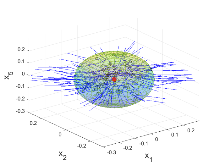
For , here the parameter is slightly different from that in the above case and . Therefore is the only equilibria of the system (8). In this case, we can also visualize a hidden chaotic set in the system (8). To verify that the set in Fig. 13b is hidden, around equilibrium , we choose a small spherical vicinity of radius and take random initial points on it (in our experiment, as in Fig. 14b). Using MATLAB, we integrate system (8) with these initial points to explore the obtained trajectories. We repeat this procedure several times in order to get different initial points for trajectories on the sphere. We get the following results: all the obtained trajectories tend to the torus and do not tend to the chaotic set (see Fig. 14a), this torus is closer55 5 The distance between the torus and the equilibria can be estimated by considering the last point on torus and plane, which contains the set of equilibria . If we consider in the point and the plane , then the distance from the point to the plane is: To determine the equation of a plane in one can consider five points, which do not lie on the same straight line. The normal vector to a plane can be obtained by taking the cross product of four vectors on this plane. In our case equation of the plane which contains the set of equilibria is: . From Fig. 13a the last point on the torus is , then the distance from this point to the plane is: . to the set of equilibria (see Fig. 13a). This gives us a reason to classify the chaotic set, obtained in the system (8), as the hidden one (see Fig. 13b).


Appendix B Localization using perpetual points
Consider system (8) as an autonomous differential equation of general form:
| (31) |
where represents the right-hand side of system (8).
The equilibrium points of a dynamical system are the ones at which the velocity and acceleration of the system simultaneously become zero. In this subsection, we state that there are points, termed as perpetual points Prasad-2015, which may help to visualize hidden attractors.
For system (31), the equilibrium points are defined by the equation . Consider a derivative of system (31) with respect to time:
| (32) |
where is the Jacobian matrix. Here, may be termed as an acceleration vector. System (32) shows the variation of acceleration in the phase space. Similar to the equilibrium points estimation, where we set the velocity vector to zero, we can also get a set of points, where in (32), i.e. the points corresponding to the zero acceleration. At these points, the velocity may be either zero or nonzero. This set includes the equilibrium points with zero velocity as well as a subset of points with nonzero velocity. These nonzero velocity points are termed as perpetual points DudkowskiJKKLP-2016; Prasad-2015; Prasad-2016.
Remark 4.
The analytical formula of the perpetual points of system (8) can not be derived, meanwhile the numerical solution of the algebraic system is , which coincide with the equilibrium , so system (8) has no perpetual points. For system (29), which structure seems simpler than the original system (8), is the only solution of the system , thus, there are also no nonzero velocity points .
Appendix C Numerical verification of basins of attraction near the zero equilibrium point
For the system (8) the eigenvalues at are: So the equilibria has 2-dimensional unstable manifold. For the fist two eigenvalues with positive real part, the corresponding eigenvectors are: and respectively. In the case of complex eigenvalues we can use the following formula to plot trajectories in a vicinity of
| (33) |
where is a constant that represent the size of the vicinity and should be small, , are real and imaginary parts of the eigenvalues respectively, is an auxiliary angle, and . Initial points of unstable manifolds of can be obtained by putting in Eq. (33) as
| (34) |
In Fig. 15 we plotted local stable, unstable manifolds of and random initial points on local 2-D unstable manifolds of . Fig. 16 shows unstable manifolds with random initial points from local 2-D unstable manifolds of (in our experiment, we choose 100 random points for the angle inside interval and fix the size of vicinity as . We repeat this procedure several times in order to get different initial points). From Fig. 16 one can see that, these unstable manifolds form by their scrolling a tube around the circle of equilibria . This experiment confirms that all trajectories which start from a vicinity of the unstable equilibria go to the circle of equilibria , and this means that the green set in Fig. 12a is not self-excited. We can do the same experiment in the case of the torus as in Fig 13b. In Fig. 17 we plotted trajectories with random initial points on local 2-D unstable manifolds of , which tend to the torus. So the green set in Fig 13b is not self-excited. In order to demonstrate separation between basins of attraction of and the green set (as in Fig. 12a) which is located between the blue tube that is formed by scrolling of these trajectories and the domain which is defined by separatricies. We need not only to separate basin of attraction of this green set from these blue manifolds, but also from trajectory going from infinity to which can be derived analytically by formula , . Because of the system (8) is 5-dimensional it is difficult to show such separation, so we can say that the green set it is possible to be an attractor.


Appendix D Numerical verification of basins of attraction around the set of equilibria
In order to numerically verify the attractiveness of the chaotic set the following numerical experiment can be used. In this experiment, we consider initial points on the various line segments in the vicinity around the set of equilibria in Figs. 12a and 13b (see Fig. 18). From Fig. 18 we can conclude the following: around the equilibria there is a vicinity such that trajectories starting from this vicinity approach equilibria and outside it approach attractor. For Fig. 13b the vertical and horizontal diagonals are considered with radius and respectively and partition step . And for the others line segments as in Figs. 18b and 18c we used the same partition step. In Fig. 19 we plotted two trajectories with initial points from blue and red parts of vertical diagonal. The same procedure can be used for Fig. 12a with vertical and horizontal diagonals have radius and respectively and partition step on all considered line segments. Fig. 20 shows two trajectories with starting points from blue and red parts of vertical diagonal. In addition, another procedure can be used to verify that the green set in Fig. 12a not fall on the circle of equilibria . Around one scroll of trajectory of an unstable manifold from its outer sides we consider line segments with length 5 and partition step 0.01 as in Fig. 21a. In Fig. 21b we plotted a trajectory with starting point from the upper outer line segment.


Appendix E Attempts to prove the attractiveness of the transient set
To demonstrate strictly the attractiveness of the green sets as in Figs. 12a and 13b, another technique can be utilized. The idea of this technique is based on the fact that the complex Lorenz system (4) has a projective space, in which the states differing only by a common phase of variables and are considered to be equivalent (see Section III).
Now, it is important to mention the following properties
of the projective system (29) VladimirovTD-1997; VladimirovTD-1998-IJBC:
(i) All physical information and dynamics in the phase space of the system (4) can be derived from the equations of motion (29) in the projective space.
(ii) The projective system (29) has a 1-dimensional unstable manifold and 3-dimensional stable manifold.
Note that the projective system (29) has the following two equilibria: and , where
The equilibria and in the projective space represent the projections of the equilibria and of the system (8) respectively. For the torus as in Fig. 13a its projection in the projective space is a limit cycle .
Because of the projection system (29) has a -dimensional unstable manifold and the projective mapping (27) preserves the ”chaoticity” of attractors. So, it is reasonable to use the projection system (29) to identify whether the chaotic sets in Figs. 12a and 13b are attractors or transient chaotic sets. For the parameters (see Fig. 12a), around the equilibria we choose a small spherical vicinity of radius 0.002 and consider 100 random initial points on it. From Fig. 22 one can observe the following: all the considered unstable manifolds of go in one direction and approach . We did the same experiment for the case of the torus and got the same conclusion (see Fig. 23).


(b) Magnification of the area around to show the sphere of random initial points and the corresponding trajectories tending to .


(b) Magnification of the area around to show the spherical of random points and the considered trajectories tending to the limit cycle .