Designing flat-band tight-binding models with tunable multifold band touching points

Consider a periodic lattice treated in the TB approximation Ashcroft and Mermin 1976, with $N$ (atomic) orbitals per unit cell, i.e. with $N$ sublattices labeled by $\alpha=A,B,C,...$ . On such a lattice, a compact localized state (CLS) centered at some localization center $\mathbf{R}_{\text{C}}$ can be formed as a linear combination

of orbitals $\ket{\alpha_i}$, where the complex number $w_{\alpha_{i}}$ – the CLS amplitude on the respective orbital – takes a nonzero value only for a finite number of lattice sites around $\mathbf{R}_{\text{C}}$. The subindex $i$ takes account of the fact that more than one orbital of a given type $\alpha$ will in general appear in the CLS (orbitals $\alpha_{i}$ and $\alpha_{j\neq i}$ are in different unit cells). Since only a finite number of orbitals contributes to the CLS, the CLS wave function

is restricted to a finite region of the lattice, with strictly zero probability amplitude outside this region.

As an example, consider the CLS built on the square lattice ($N=2$) shown in Fig. 2(a).

It involves four orbitals labeled by $\alpha=A,B$ and $i=1,2$, i.e.

Similarly, the CLS on the Kagome lattice ($N=3$) shown in Fig. 2(b) involves six orbitals, i.e.

The orbitals with nonzero amplitude ($w_{\alpha_{i}}\neq 0$) are located at positions $\smash{\boldsymbol{\delta}_{\alpha_{i}}}$ as measured from $\mathbf{R}_{\text{C}}$. For the CLS of panel (a), we have $\smash{\boldsymbol{\delta}_{A_{1,2}}=\mp\frac{1}{2}}(1,-1)$ and $\smash{\boldsymbol{\delta}_{B_{1,2}}=\mp\frac{1}{2}}(1,1)$. For the CLS of panel (b), the positions are $\smash{\boldsymbol{\delta}_{A_{1,2}}=\mp\frac{1}{2}}(1,-\sqrt{3})$, $\smash{\boldsymbol{\delta}_{B_{1,2}}=\pm\frac{1}{2}}(1,\sqrt{3})$, and $\smash{\boldsymbol{\delta}_{C_{1,2}}=\pm(1,0)}$. Note that the lattice constant is taken as $a=1$ here and throughout.

For any CLS (1) centered at some $\mathbf{R}_{\text{C}}$, there exists a macroscopic number of equivalent copies translated by some Bravais vector. Thus, for any given CLS, we can introduce a Bloch state of the CLS (BCLS) $\ket{f_\mathbf{k}}$, which is obtained as an unnormalized superposition of the CLS and all its translated copies:

Note that the (reciprocal-space) BCLS is simply the Fourier transform of the (real-space) CLS. In the second line of Eq. (5), $\ket{\alpha,\mathbf{k}}$ are Bloch basis states ¹¹ 1 The Bloch basis states used here may be written as $\ket{\alpha,\mathbf{k}}\equiv\mathcal{N}^{-1/2}\sum_{m}e^{-i\mathbf{k}\cdot(\mathbf{R}_{m}+\mathbf{r}_{\alpha})}\ket{m,\alpha}$. The sum $\sum_{m}$ runs over all lattice vectors, $\mathcal{N}$ is the total number of unit cells and $\mathbf{R}_{m}+\mathbf{r}_{\alpha}$ is the position vector of the orbital $\ket{m,\alpha}$, i.e. the orbital of type $\alpha$ in unit cell $m$. Note that the BCLS was introduced in a similar way in Ref. Rhim and Yang 2019, where the authors work in the ”tight-binding basis I” such that the Bloch Hamiltonian has the periodicity of the FBZ. In contrast, here we work in the ”tight-binding basis II” Bena and Montambaux 2009. and

is completely specified by the positions and amplitudes of the orbitals contained in the associated real-space CLS. Hereafter, we work in the Bloch basis, where the BCLS takes the form of a column vector:

For example, the CLS of Fig. 2(a) gives rise to a BCLS

and the CLS of Fig. 2(b) corresponds to a BCLS

where $k_{\pm}\equiv\frac{1}{2}(k_{x}\pm\sqrt{3}k_{y})$. In the same way, each arbitrarily designed CLS on any lattice uniquely corresponds to some BCLS $\ket{f_\mathbf{k}}$; the latter is an important quantity in our flat-band construction scheme, cf. Fig. 1.

Note that $\ket{f_\mathbf{k}}$ is called singular if there exists a point $\mathbf{k}_{0}$ in the FBZ such that $\ket{f_{\mathbf{k}_0}}=0$, while it is called non-singular otherwise Rhim and Yang 2019. The (non-)singularity of $\ket{f_\mathbf{k}}$ is a useful tool for characterizing the properties of BTPs at the flat-band energy.

We now argue that for any arbitrarily shaped (input) CLS on any periodic lattice, it is possible to construct families of tight-binding Hamiltonians $H$ such that this CLS and all its translated copies constitute a macroscopically degenerate set of eigenstates:

In order to find these tight-binding Hamiltonians $H$, the strategy adopted in this work consists in designing Bloch Hamiltonians $H_{\mathbf{k}}$ ($N\times N$ matrices) for which the BCLS $\ket{f_\mathbf{k}}$ associated to the input CLS represents a flat-band eigenstate:

Once such matrices $H_{\mathbf{k}}$ are found, it is straightforward to obtain the real-space models $H$ from them. Hereafter, we will take $\epsilon_{0}=0$ without loss of generality.

To see how this Bloch Hamiltonian design can be done, let us write Eq. (11) explicitly in matrix form:

Evidently, a flat band will automatically exist if the Bloch Hamiltonian is imposed to be an appropriate function $H_{\mathbf{k}}(\ket{f_\mathbf{k}})$ of the BCLS. More concretely, the matrix elements $H_{\mathbf{k},\alpha\beta}$ should depend on the components $f_{\alpha}(\mathbf{k})$ in such a way that $\sum_{\beta}H_{\mathbf{k},\alpha\beta}f_{\beta}(\mathbf{k})=0$ is fulfilled for every $\alpha$, independently of the detailed functional form of the components $f_{\alpha}(\mathbf{k})$.

Thus, the task at hand consists in finding matrices $H_{\mathbf{k}}(\ket{f_\mathbf{k}})$ that fulfill Eq. (12). However, we have to be aware of an additional physical constraint:

This means that $H_{\mathbf{k}}(\ket{f_\mathbf{k}})$ has to be chosen such that the real-space TB Hamiltonian $H$ constructed from it makes sense on a lattice. The latter property is not automatically guaranteed for all matrices $H_{\mathbf{k}}(\ket{f_\mathbf{k}})$ that fulfill Eq. (12). More concretely, for $H_{\mathbf{k}}$ to be reasonable, the matrix elements $H_{\mathbf{k},\alpha\beta}$ should be made of finite sums of Bloch phases that are compatible with the underlying lattice geometry (see Appendix A for more details).

As it turns out, there are two different simple choices for matrices that fulfill condition (12):

Designing quadratic Hamiltonians is possible for $N\geq 2$ and, conveniently, condition (13) is automatically fulfilled for any input CLS. In contrast, designing linear Hamiltonians requires $N\geq 3$ and condition (13) is only fulfilled for special input CLSs. For this reason, the quadratic case may be regarded as simpler and will be treated first.

Consider some CLS built on a lattice with two orbitals per unit cell:

The corresponding BCLS has two components,

where hereafter $f_{\alpha}\equiv f_{\alpha}(\mathbf{k})$ for brevity. We now want to construct a matrix $H_{\mathbf{k}}$ that vanishes on $\ket{f_\mathbf{k}}$ (i.e. $H_{\mathbf{k}}\ket{f_\mathbf{k}}=0$). The only generic way to do this consists in introducing a state

orthogonal to $\ket{f_\mathbf{k}}$, as well as the matrix

Then a Bloch Hamiltonian defined as

will obviously have $\ket{f_\mathbf{k}}$ as an eigenstate of zero energy; in other words, Eq. (12) is fulfilled for any $\ket{f_\mathbf{k}}$. The band structure associated to Eq. (18) reads

Here, $\lambda^{AB}_{\mathbf{k}}$ is an arbitrary real function with the periodicity of the FBZ. If it is taken positive (or negative) throughout, the flat band is gapped away from the dispersive band at all $\mathbf{k}$-points where $\ket{f_\mathbf{k}}$ does not vanish, i.e. only singular BTPs Rhim and Yang 2019 can occur. In contrast, if $\lambda^{AB}_{\mathbf{k}}$ changes sign in the FBZ, non-singular BTPs are possible. Since we are predominantly interested in nontrivial BTPs created by the singularity of the flat-band eigenstate, we will take $\lambda^{AB}_{\mathbf{k}}=1$ from now on.

Let us now see how flat-band TB models can be designed from Eq. (18). As a first example, consider again the CLS used previously, cf. Fig. 3(a).

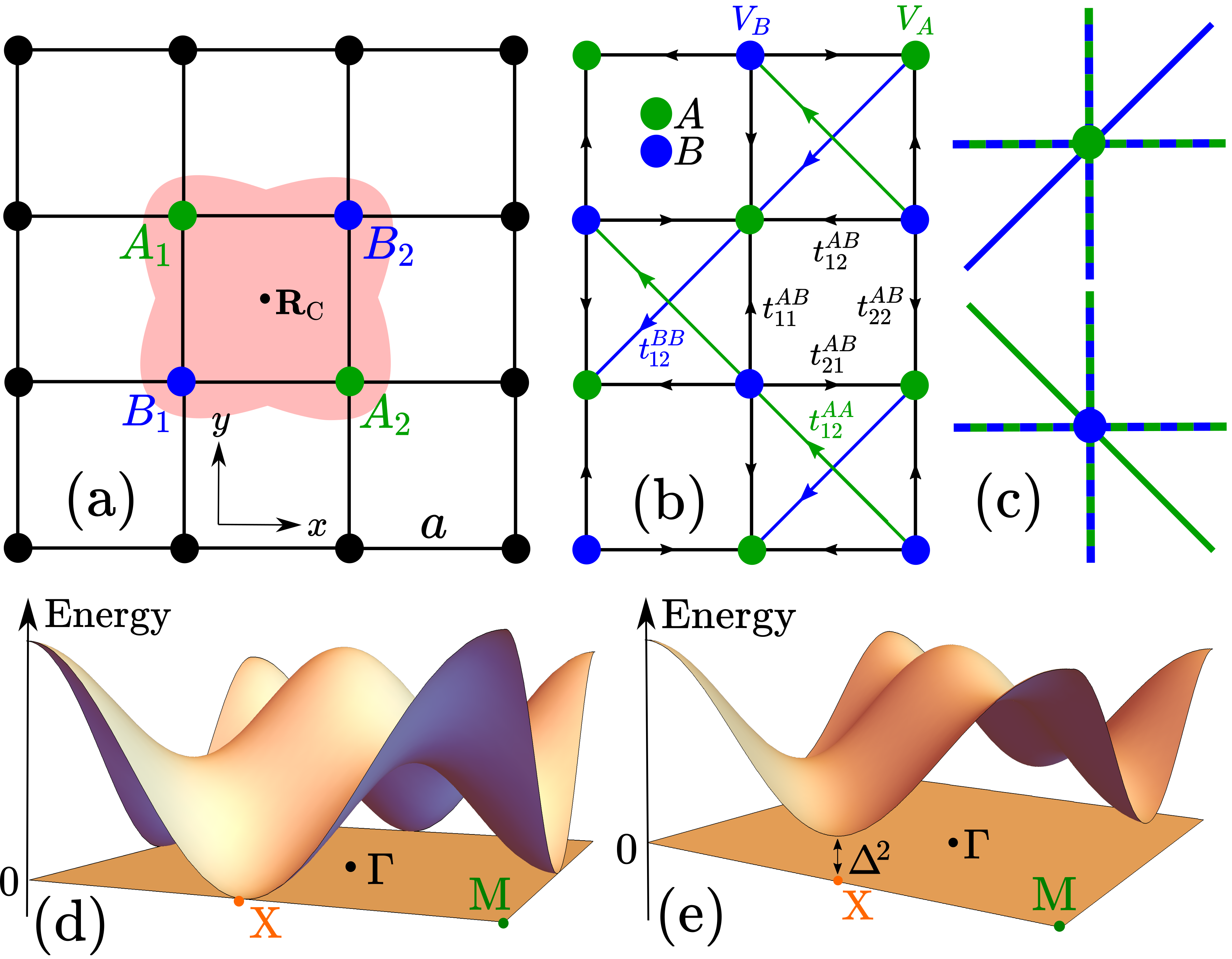
We now simply insert the corresponding BCLS (8) into the Bloch Hamiltonian (18), to obtain

where

The real-space TB model $H$ described by this Bloch Hamiltonian is depicted in Fig. 3(b). The hopping directions that appear can be directly understood from the shape of the CLS, as illustrated in Fig. 3(c): hoppings from site $A$ to site $B$ ($B$ to $A$, $A$ to $A$, $B$ to $B$) are determined by all vectors that connect orbitals $A$ to orbitals $B$ ($B$ to $A$, $B$ to $B$, $A$ to $A$) within the CLS (see Appendix A for details). As a consequence, the model (21) involves first- and second-neighbor hoppings.

The onsite energies $V_{A}\equiv|w_{B_{1}}|^{2}+|w_{B_{2}}|^{2}$, $V_{B}\equiv|w_{A_{1}}|^{2}+|w_{A_{2}}|^{2}$, inter-sublattice hopping parameters $t_{ij}^{\alpha\beta}\equiv-w_{\alpha_{i}}w_{\beta_{j}}^{*}$ and intra-sublattice hopping parameters $t_{ij}^{\alpha\alpha}\equiv w_{\alpha_{i}}w_{\alpha_{j}}^{*}$ strongly depend on the CLS amplitudes. As a consequence, the band structure can be engineered by the choice of the CLS amplitudes. In particular, the existence of a (singular) BTP can be ensured by choosing $\ket{f_\mathbf{k}}$ singular. For example, if the CLS amplitudes are such that $\ket{f_{\mathbf{k}_\text{X}}}=0$, a BTP at the X point of the FBZ appears, see Fig. 3(d). Similarly, there would be a BTP at the $\Gamma$ point if $w_{\alpha_{1}}=-w_{\alpha_{2}}\in\mathbb{R}$. In contrast, if $\ket{f_\mathbf{k}}$ is chosen non-singular, the bands are gapped away from each other, see Fig. 3(e).

As a second example, consider the CLS on the honeycomb lattice shown in Fig. 4(a). It is straightforward to obtain the BCLS

where again $k_{\pm}\equiv(k_{x}\pm\sqrt{3}k_{y})/2$. Inserting into Eq. (18), one obtains a TB model of the form (20), where now

with onsite energies and hoppings as defined above. This TB model is shown in Fig. 4(b). Due to the asymmetric shape of the input CLS, the hoppings are also distributed asymmetrically, as illustrated in Fig. 4(c). By an appropriate choice of the CLS amplitudes, the band structure can be freely designed to exhibit a BTP at the $\Gamma$ point or at the K points, see Fig. 4(d)&(e), or to be gapped by taking $\ket{f_\mathbf{k}}$ non-singular.

Proceeding in the same way, infinitely many different $N=2$ flat-band models and their band structures can be designed. For any imaginable CLS (14), if one inserts the corresponding BCLS (15) into Eq. (18), one obtains a flat-band TB model with hopping directions that are determined by the shape of the CLS (i.e. the set of all vectors $\boldsymbol{\delta}_{\alpha_{i}}$), and hopping parameters as well as onsite energies that are determined by the CLS amplitudes $w_{\alpha_{i}}$.

As explained in more detail in Appendix A, the Bloch Hamiltonian (18) is indeed always reasonable [cf. condition (13)] due to its quadratic character. In fact, it is not only a reasonable flat-band Hamiltonian, but the only possible form for the Bloch Hamiltonian of any $N=2$ flat-band model. This was already anticipated by Rhim and Yang Rhim and Yang 2019 and can be easily understood from the spectral theorem, see Appendix B.

To illustrate that the procedure outlined above indeed works for arbitrarily complicated input CLSs, we may consider the snowflake-shaped CLS displayed in Fig. 4(f). Of course, for such an extended input CLS, the real-space model that one obtains involves many further-neighbor hoppings and it is not useful to draw it explicitly. However, conveniently, the band structure (19) can be analyzed and designed before considering the real-space model. For example, taking $\smash{w_{\alpha_{i}}=1}$ for all 42 orbitals involved in the CLS, the dispersive band $\epsilon_{1}(\mathbf{k})$ strongly oscillates and exhibits a large peak at the $\Gamma$ point (not shown). If the amplitudes are flipped to $\smash{w_{\alpha_{i}}=-1}$ on three out of the six branches of the snowflake, see Fig. 4(g), then $\epsilon_{1}(\mathbf{k})$ exhibits six peaks arrayed hexagonally in the FBZ.

As we will show, an analogous procedure of flat-band model and band structure design is possible for $N>2$. Additionally, the tunability turns out to be considerably increased.

Consider now a CLS built on a lattice with three orbitals per unit cell:

The corresponding BCLS has three components,

We can now introduce three states orthogonal to $\ket{f_\mathbf{k}}$, namely

with corresponding matrices

A class of flat-band Bloch Hamiltonians is then obtained as a linear combination:

where $\lambda_{\mathbf{k}}^{AB}$, $\lambda_{\mathbf{k}}^{AC}$, $\lambda_{\mathbf{k}}^{BC}$ are arbitrary real functions with the periodicity of the FBZ. It will suffice to choose them as constants, $\lambda_{\mathbf{k}}^{\alpha\beta}=\lambda_{\alpha\beta}$.

The Hamiltonian (28) is analogous to Eq. (18) in that it automatically verifies the desired conditions (12) & (13) for any conceivable input CLS, i.e. for any $\ket{f_\mathbf{k}}$. Therefore, infinitely many flat-band models on any $N=3$ lattice can be obtained from Eq. (28).

Moreover, there is an additional advantage compared to the $N=2$ case, namely there are now three relative parameters $\lambda_{\alpha\beta}$, while the single parameter $\lambda_{AB}$ in the two-band Hamiltonian (18) only acts globally. As a consequence, the Hamiltonian (28) can be strongly tuned even if an input CLS completely fixed with regard to both shape and amplitudes is used. This represents an additional degree of freedom absent in the two-band case. In this context, it is crucial to realize that the states (26) are not eigenstates of the Hamiltonian (28). In fact, they form an overcomplete basis of the space orthogonal to $\ket{f_\mathbf{k}}$. This redundancy is at the origin of the tunability provided by the $\lambda_{\alpha\beta}$. In contrast to the flat-band eigenstate $\ket{f_\mathbf{k}}$, the dispersive-band eigenstates of the Hamiltonian (28) do depend on the parameters $\lambda_{\alpha\beta}$.

The dependency on the choice of the input CLS (i.e. of the functions $f_{\alpha}$) and the tunability by the $\lambda_{\alpha\beta}$ are clearly reflected in the Hamiltonian’s band structure

where $C_{n}\equiv\Tr(H^n_\mathbf{k})$ are given by

As an example, consider again the six-site CLS on the Kagome lattice used previously, shown in Fig. 5(a), with corresponding BCLS (9).

Inserting into Eq. (28), one obtains a flat-band TB model

with diagonal matrix elements

and off-diagonal elements

Again, the hopping directions are determined by the CLS shape, as illustrated in Fig. 5(b), and the TB model thus involves at most third-neighbor hoppings.

The onsite energies $V_{\alpha}\equiv\sum_{\beta\neq\alpha}\lambda_{\alpha\beta}(|w_{\beta_{1}}|^{2}+|w_{\beta_{2}}|^{2})$, inter-sublattice hoppings $t_{ij}^{\alpha\beta}\equiv-\lambda_{\alpha\beta}w_{\alpha_{i}}w_{\beta_{j}}^{*}$ and intra-sublattice hoppings $t_{ij}^{\alpha,\beta\beta}\equiv\lambda_{\alpha\beta}w_{\beta_{i}}w_{\beta_{j}}^{*}$ are strongly tunable by the six CLS amplitudes $w_{\alpha_{i}}$ and the three parameters $\lambda_{\alpha\beta}$. This affords considerable control over the behavior of the dispersive bands, and in particular over the occurrence of BTPs. For example, the band structure can be chosen to exhibit a BTP at the $\Gamma$ point, and the position of the flat band with respect to the dispersive bands can be controlled by the $\lambda_{\alpha\beta}$, see Fig. 5(c)&(d). Similarly, the BTP can be placed at the K points, and again the position of the flat band can be controlled, see Fig. 5(e)&(f). Of course, the flat band can also be gapped out completely by an imbalance in the CLS amplitudes.

More generally, for three-band models of the form (28), a BTP of any degeneracy, and at various positions in the FBZ, can be designed without destroying the flat band. At $\mathbf{k}=\mathbf{k}_{0}$, there will be a twofold BTP if $2C_{2}(\mathbf{k}_{0})=C_{1}(\mathbf{k}_{0})[1+C_{1}(\mathbf{k}_{0})]$, and a threefold BTP if $C_{1}(\mathbf{k}_{0})=C_{2}(\mathbf{k}_{0})=0$. Clearly, this can be achieved in several different ways, with or without fine-tuning of the $\lambda_{\alpha\beta}$. All possible scenarios are listed in Appendix C.

The arguments made above can be readily extended to any $N$. Consider a generic CLS (1) built on a lattice with $N$ orbitals per unit cell, with corresponding BCLS

We may now introduce $\binom{N}{2}$ states

orthogonal to $\ket{f_\mathbf{k}}$, and the $N\times N$ matrices

constructed from them. A generic quadratic flat-band Bloch Hamiltonian is then obtained by forming a linear combination of these $\binom{N}{2}$ matrices:

where $\alpha,\beta\in\{A,B,C,...\}$ and $\lambda^{\alpha\beta}_{\mathbf{k}}$ is an arbitrary real function with the periodicity of the FBZ. We will assume $\lambda^{\alpha\beta}_{\mathbf{k}}=\lambda_{\alpha\beta}$, such that the off-diagonal and diagonal matrix elements of the Hamiltonian (37) explicitly read

The Hamiltonian (37), which generalizes Eqs. (18) & (28) to any $N$, is the first main result of this paper. One can insert into it any arbitrary CLS built on any lattice, for any spatial dimension and any number of sites per unit cell. Since conditions (12) & (13) are automatically fulfilled, each such input CLS gives rise to a reasonable real-space tight-binding model with a flat band. One thus obtains arbitrarily many flat-band models on any lattice.

Of course, while Eq. (37) provides infinitely many flat-band models, it does not capture all possible flat-band models except in the $N=2$ limit. In particular, flat-band models with a linear function $H_{\mathbf{k}}(\ket{f_\mathbf{k}})$ exist for $N\geq 3$, see Section IV.

The flat-band models obtained from Eq. (37) are tunable by two independent knobs: the functions $f_{\alpha}$ and the $N(N-1)/2$ parameters $\lambda_{\alpha\beta}$. The latter tunability stems from the fact that the states (35) are not eigenstates of the Hamiltonian (37) and form an overcomplete basis of the space orthogonal to $\ket{f_\mathbf{k}}$.

Although, for $N>3$, there is no elegant closed-form solution for the energy bands, the existence of a flat band is always guaranteed, and BTPs with any degree of degeneracy ($d=1,...,N$) can be designed. The two most interesting classes of BTPs (not requiring fine-tuning of the $\lambda_{\alpha\beta}$) are the following. (1) If $\ket{f_{\mathbf{k}_0}}=0$ for some $\mathbf{k}_{0}$, there will be an $N$-fold (singular) BTP at $\mathbf{k}_{0}$. We have already seen examples for this in the two-band and three-band case, cf. Figs. 3–5. (2) If, at $\mathbf{k}_{0}$, all except one component of $\ket{f_{\mathbf{k}_0}}$ vanish, say $f_{\alpha_{0}}(\mathbf{k}_{0})\neq 0$ and $f_{\alpha\neq\alpha_{0}}(\mathbf{k}_{0})=0$, then the Hamiltonian (37) becomes locally diagonal with eigenvalues $\{0,\lambda_{\alpha_{0},\alpha\neq\alpha_{0}}|f_{\alpha_{0}}(\mathbf{k}_{0})|^{2}\}$. In other words, a $d$-fold BTP at $\mathbf{k}_{0}$, with $1\leq d\leq N-1$, can be created as desired by setting $d-1$ parameters $\lambda_{\alpha_{0},\alpha\neq\alpha_{0}}$ to zero.

As an example for the $N>3$ case, consider a CLS on an $N=4$ bilayer honeycomb lattice, shown in Fig. 6(a).

For simplicity, we take all CLS amplitudes to be identical, $w_{\alpha_{i}}=1$. The corresponding BCLS is given by

Even though the CLS is completely fixed (shape and amplitudes), the flat-band Bloch Hamiltonian (37) built from it is still tunable by six parameters $\lambda_{AB},\lambda_{AC},\lambda_{AD},\lambda_{BC},\lambda_{BD},\lambda_{CD}$. To reduce the number of parameters, it is reasonable to set $\lambda_{CD}=\lambda_{AB}$, $\lambda_{BC}=\lambda_{AD}$ and $\lambda_{BD}=\lambda_{AC}$ for reasons of symmetry [cf. Fig. 6(a)]. We may then further set $\lambda_{AC}=-c_{\theta}^{2}\lambda_{AB}$ and $\lambda_{AD}=-s_{\theta}^{2}\lambda_{AB}$ to ensure a tight-binding model with zero onsite energies and no intra-sublattice hopping:

Here, the shorthand notation $s_{\theta}\equiv\sin\theta$ and $c_{\theta}\equiv\cos\theta$ is used. Physically, the parameter $\theta$ quantifies the ratio between vertical ($AC$ and $BD$) and diagonal ($AD$ and $BC$) inter-layer hoppings. The band structure of the model (40) reads

in units of $\lambda_{AB}$. The upper two (lower two) bands are tunable by $\theta$ if $\lambda_{AB}$ is taken to be positive (negative), as shown in Fig. 6(b)–(e). Note that the system has a chiral symmetry for $\theta=n\pi/2$, $n\in\mathbb{Z}$. In this case there is a doubly degenerate flat band, of which one is essential ($\epsilon_{0}$) while the other one is accidental ($\epsilon_{2}$ or $\epsilon_{3}$).

Finally, to illustrate that our flat-band model construction scheme indeed works for any dimension, an $N=4$ flat-band model built from a CLS on the (3D) cubic lattice is discussed in Appendix D.

Consider again some CLS built on a lattice with three orbitals per unit cell:

with corresponding BCLS

Our goal is now to construct $N=3$ flat-band Bloch Hamiltonians $H_{\mathbf{k}}$ that are linear functions of $\ket{f_\mathbf{k}}$. To achieve this, one cannot use a completely arbitrary input CLS, in contrast to the quadratic scenario. Instead, the CLS needs to have special properties.

We can identify two classes of CLSs that allow to build a linear $H_{\mathbf{k}}$. More specifically, CLSs belonging to the first class may be called chiral CLSs, since the flat-band Bloch Hamiltonians built from them are characterized by an effective (global) chiral symmetry Ryu et al. 2010

with a unitary matrix $\mathcal{S}$ that fulfills $\mathcal{S}^{2}=\mathbf{1}_{3}$. As it turns out, in the class of chiral CLSs we can further distinguish between a type-I chiral CLS (C_I-CLS), in which case $f_{A}f_{B}f_{C}=0$, and a type-II chiral CLS (C_II-CLS), in which case $f_{A}f_{B}f_{C}\neq 0$. Similarly, CLSs belonging to the second class may be called CP-CLSs, since they give rise to flat-band Bloch Hamiltonians that exhibit an effective (global) CP symmetry

References

- Ashcroft and Mermin (1976) N. W. Ashcroft and N. D. Mermin, Solid State Physics (Holt, Rinehart and Winston, New York, 1976).
- Joannopoulos et al. (2011) J. Joannopoulos, S. Johnson, J. Winn, and R. Meade, Photonic Crystals: Molding the Flow of Light - Second Edition (Princeton University Press, 2011).
- Landau (1930) L. Landau, Diamagnetismus der Metalle, Zeitschrift für Physik 64, 629 (1930).
- Sutherland (1986) B. Sutherland, Localization of electronic wave functions due to local topology, Phys. Rev. B 34, 5208 (1986).
- Lieb (1989) E. H. Lieb, Two theorems on the Hubbard model, Phys. Rev. Lett. 62, 1201 (1989).
- Mielke (1991a) A. Mielke, Ferromagnetic ground states for the Hubbard model on line graphs, Journal of Physics A: Mathematical and General 24, L73 (1991a).
- Mielke (1991b) A. Mielke, Ferromagnetism in the Hubbard model on line graphs and further considerations, Journal of Physics A: Mathematical and General 24, 3311 (1991b).
- Tasaki (1992) H. Tasaki, Ferromagnetism in the Hubbard models with degenerate single-electron ground states, Phys. Rev. Lett. 69, 1608 (1992).
- Girvin (2005) S. M. Girvin, Introduction to the Fractional Quantum Hall Effect, in The Quantum Hall Effect: Poincaré Seminar 2004, edited by B. Douçot, V. Pasquier, B. Duplantier, and V. Rivasseau (Birkhäuser Basel, 2005) pp. 133–162.
- Monarkha and Syvokon (2012) Y. P. Monarkha and V. E. Syvokon, A two-dimensional Wigner crystal (Review Article), Low Temperature Physics 38, 1067 (2012).
- Tasaki (1998) H. Tasaki, From Nagaoka’s Ferromagnetism to Flat-Band Ferromagnetism and Beyond: An Introduction to Ferromagnetism in the Hubbard Model, Progress of Theoretical Physics 99, 489 (1998).
- Derzhko et al. (2015) O. Derzhko, J. Richter, and M. Maksymenko, Strongly correlated flat-band systems: The route from Heisenberg spins to Hubbard electrons, International Journal of Modern Physics B 29, 1530007 (2015).
- Liu et al. (2014) Z. Liu, F. Liu, and Y.-S. Wu, Exotic electronic states in the world of flat bands: From theory to material, Chinese Physics B 23, 077308 (2014).
- Leykam et al. (2018) D. Leykam, A. Andreanov, and S. Flach, Artificial flat band systems: from lattice models to experiments, Advances in Physics: X 3, 1473052 (2018).
- Lin et al. (2018) Z. Lin, J.-H. Choi, Q. Zhang, W. Qin, S. Yi, P. Wang, L. Li, Y. Wang, H. Zhang, Z. Sun, L. Wei, S. Zhang, T. Guo, Q. Lu, J.-H. Cho, C. Zeng, and Z. Zhang, Flatbands and Emergent Ferromagnetic Ordering in Kagome Lattices, Phys. Rev. Lett. 121, 096401 (2018).
- Kang et al. (2020) M. Kang, L. Ye, S. Fang, J.-S. You, A. Levitan, M. Han, J. I. Facio, C. Jozwiak, A. Bostwick, E. Rotenberg, M. K. Chan, R. D. McDonald, D. Graf, K. Kaznatcheev, E. Vescovo, D. C. Bell, E. Kaxiras, J. van den Brink, M. Richter, M. Prasad Ghimire, J. G. Checkelsky, and R. Comin, Dirac fermions and flat bands in the ideal kagome metal FeSn, Nature Materials 19, 163 (2020).
- Liu et al. (2020) Z. Liu, M. Li, Q. Wang, G. Wang, C. Wen, K. Jiang, X. Lu, S. Yan, Y. Huang, D. Shen, J.-X. Yin, Z. Wang, Z. Yin, H. Lei, and S. Wang, Orbital-selective Dirac fermions and extremely flat bands in frustrated kagome-lattice metal CoSn, Nature Communications 11, 4002 (2020).
- Cheng et al. (2019) Y. Cheng, C. Huang, H. Hong, Z. Zhao, and K. Liu, Emerging properties of two-dimensional twisted bilayer materials, Chinese Physics B 28, 107304 (2019).
- Andrei and MacDonald (2020) E. Y. Andrei and A. H. MacDonald, Graphene bilayers with a twist, Nature Materials 19, 1265–1275 (2020).
- Mogera and Kulkarni (2020) U. Mogera and G. U. Kulkarni, A new twist in graphene research: Twisted graphene, Carbon 156, 470 (2020).
- Miyahara et al. (2005) S. Miyahara, K. Kubo, H. Ono, Y. Shimomura, and N. Furukawa, Flat-Bands on Partial Line Graphs – Systematic Method for Generating Flat-Band Lattice Structure, Journal of the Physical Society of Japan 74, 1918 (2005).
- Röntgen et al. (2018) M. Röntgen, C. V. Morfonios, and P. Schmelcher, Compact localized states and flat bands from local symmetry partitioning, Phys. Rev. B 97, 035161 (2018).
- Morfonios et al. (2021) C. V. Morfonios, M. Röntgen, M. Pyzh, and P. Schmelcher, Flat bands by latent symmetry, Phys. Rev. B 104, 035105 (2021).
- Dias and Gouveia (2015) R. G. Dias and J. D. Gouveia, Origami rules for the construction of localized eigenstates of the Hubbard model in decorated lattices, Scientific Reports 5, 16852 (2015).
- Morales-Inostroza and Vicencio (2016) L. Morales-Inostroza and R. A. Vicencio, Simple method to construct flat-band lattices, Phys. Rev. A 94, 043831 (2016).
- Ramachandran et al. (2017) A. Ramachandran, A. Andreanov, and S. Flach, Chiral flat bands: Existence, engineering, and stability, Phys. Rev. B 96, 161104 (2017).
- Călugăru et al. (2021) D. Călugăru, A. Chew, L. Elcoro, N. Regnault, Z.-D. Song, and B. A. Bernevig, General Construction and Topological Classification of All Magnetic and Non-Magnetic Flat Bands (2021), arXiv:2106.05272 .
- Toikka and Andreanov (2018) L. A. Toikka and A. Andreanov, Necessary and sufficient conditions for flat bands in -dimensional -band lattices with complex-valued nearest-neighbour hopping, Journal of Physics A: Mathematical and Theoretical 52, 02LT04 (2018).
- Ogata et al. (2021) T. Ogata, M. Kawamura, and T. Ozaki, Methods for constructing parameter-dependent flat-band lattices, Phys. Rev. B 103, 205119 (2021).
- Mizoguchi and Udagawa (2019) T. Mizoguchi and M. Udagawa, Flat-band engineering in tight-binding models: Beyond the nearest-neighbor hopping, Phys. Rev. B 99, 235118 (2019).
- Lee et al. (2019) C.-C. Lee, A. Fleurence, Y. Yamada-Takamura, and T. Ozaki, Hidden mechanism for embedding the flat bands of Lieb, kagome, and checkerboard lattices in other structures, Phys. Rev. B 100, 045150 (2019).
- Aoki et al. (1996) H. Aoki, M. Ando, and H. Matsumura, Hofstadter butterflies for flat bands, Phys. Rev. B 54, R17296 (1996).
- Nishino et al. (2003) S. Nishino, M. Goda, and K. Kusakabe, Flat Bands of a Tight-Binding Electronic System with Hexagonal Structure, Journal of the Physical Society of Japan 72, 2015 (2003).
- Nishino and Goda (2005) S. Nishino and M. Goda, Three-dimensional Flat-Band Models, Journal of the Physical Society of Japan 74, 393 (2005).
- Flach et al. (2014) S. Flach, D. Leykam, J. D. Bodyfelt, P. Matthies, and A. S. Desyatnikov, Detangling flat bands into Fano lattices, EPL (Europhysics Letters) 105, 30001 (2014).
- Maimaiti et al. (2017) W. Maimaiti, A. Andreanov, H. C. Park, O. Gendelman, and S. Flach, Compact localized states and flat-band generators in one dimension, Phys. Rev. B 95, 115135 (2017).
- Maimaiti et al. (2019) W. Maimaiti, S. Flach, and A. Andreanov, Universal flat band generator from compact localized states, Phys. Rev. B 99, 125129 (2019).
- Rhim and Yang (2019) J.-W. Rhim and B.-J. Yang, Classification of flat bands according to the band-crossing singularity of Bloch wave functions, Phys. Rev. B 99, 045107 (2019).
- Maimaiti et al. (2021) W. Maimaiti, A. Andreanov, and S. Flach, Flat-band generator in two dimensions, Phys. Rev. B 103, 165116 (2021).
- Sathe et al. (2021) P. Sathe, F. Harper, and R. Roy, Compactly supported Wannier functions and strictly local projectors, Journal of Physics A: Mathematical and Theoretical 54, 335302 (2021).
- Castro Neto et al. (2009) A. H. Castro Neto, F. Guinea, N. M. R. Peres, K. S. Novoselov, and A. K. Geim, The electronic properties of graphene, Rev. Mod. Phys. 81, 109 (2009).
- Armitage et al. (2018) N. P. Armitage, E. J. Mele, and A. Vishwanath, Weyl and Dirac semimetals in three-dimensional solids, Rev. Mod. Phys. 90, 015001 (2018).
- Ashida et al. (2020) Y. Ashida, Z. Gong, and M. Ueda, Non-hermitian physics, Advances in Physics 69, 249 (2020).
- Bergman et al. (2008) D. L. Bergman, C. Wu, and L. Balents, Band touching from real-space topology in frustrated hopping models, Phys. Rev. B 78, 125104 (2008).
- Mizoguchi and Hatsugai (2019) T. Mizoguchi and Y. Hatsugai, Molecular-orbital representation of generic flat-band models, EPL (Europhysics Letters) 127, 47001 (2019).
- (46) The Bloch basis states used here may be written as . The sum runs over all lattice vectors, is the total number of unit cells and is the position vector of the orbital , i.e. the orbital of type in unit cell . Note that the BCLS was introduced in a similar way in Ref. Rhim and Yang 2019, where the authors work in the ”tight-binding basis I” such that the Bloch Hamiltonian has the periodicity of the FBZ. In contrast, here we work in the ”tight-binding basis II” Bena and Montambaux 2009.
- Ryu et al. (2010) S. Ryu, A. P. Schnyder, A. Furusaki, and A. W. W. Ludwig, Topological insulators and superconductors: tenfold way and dimensional hierarchy, New Journal of Physics 12, 065010 (2010).
- Green et al. (2010) D. Green, L. Santos, and C. Chamon, Isolated flat bands and spin-1 conical bands in two-dimensional lattices, Phys. Rev. B 82, 075104 (2010).
- Chen et al. (2014) L. Chen, T. Mazaheri, A. Seidel, and X. Tang, The impossibility of exactly flat non-trivial Chern bands in strictly local periodic tight binding models, Journal of Physics A: Mathematical and Theoretical 47, 152001 (2014).
- Graf and Piéchon (2021) A. Graf and F. Piéchon, Berry curvature and quantum metric in -band systems: An eigenprojector approach, Phys. Rev. B 104, 085114 (2021).
- Hwang et al. (2021) Y. Hwang, J.-W. Rhim, and B.-J. Yang, General construction of flat bands with and without band crossings based on wave function singularity, Phys. Rev. B 104, 085144 (2021).
- Bena and Montambaux (2009) C. Bena and G. Montambaux, Remarks on the tight-binding model of graphene, New Journal of Physics 11, 095003 (2009).