Learning and Generalization in Overparameterized Normalizing Flows
Kulin Shah Amit Deshpande Navin Goyal
Microsoft Research India Microsoft Research India Microsoft Research India
Abstract
In supervised learning, it is known that overparameterized neural networks with one hidden layer provably and efficiently learn and generalize, when trained using stochastic gradient descent with a sufficiently small learning rate and suitable initialization. In contrast, the benefit of overparameterization in unsupervised learning is not well understood. Normalizing flows (NFs) constitute an important class of models in unsupervised learning for sampling and density estimation. In this paper, we theoretically and empirically analyze these models when the underlying neural network is a one-hidden-layer overparametrized network. Our main contributions are two-fold: (1) On the one hand, we provide theoretical and empirical evidence that for constrained NFs (this class of NFs underlies many NF constructions) with the one-hidden-layer network, overparametrization hurts training. (2) On the other hand, we prove that unconstrained NFs, a recently introduced model, can efficiently learn any reasonable data distribution under minimal assumptions when the underlying network is overparametrized and has one hidden-layer.
1 Introduction
Neural network models trained using gradient-based algorithms have been very effective in both supervised and unsupervised learning. This is surprising for two reasons: First, the optimization of training loss is typically non-smooth and non-convex and yet gradient-based methods often succeed in making the training loss very small. Second, even large neural networks whose number of parameters are more than the size of training data often generalize well on the unseen test data, instead of overfitting the seen training data. Recent work in supervised learning attempts to theoretically analyze these phenomena.
In supervised learning, the empirical risk minimization with quadratic or cross-entropy loss is a non-convex optimization problem even for one hidden layer fully connected network. In the last few years, it was realized that when the network is overparametrized, i.e. the hidden-layer size is large compared to the dataset size or some measure of complexity of the data, one can provably show efficient training and generalization for these networks. This hinges on the fact that overparametrization makes the optimization problem close to a convex one. See, e.g., Jacot et al. 2018, Du et al. 2018, Allen-Zhu et al. 2019, Zou et al. 2020, Arora et al. 2019.
The role of overparameterization and its effect on provable training and generalization guarantees for neural networks is far less understood in unsupervised learning. Generative modeling of a probability distribution when we are given samples drawn from that distribution is an important, classical problem in statistics and unsupervised learning. The goal of a generative model is to generate new samples from the distribution and give a probability density estimate at any queried point. Popular categories of generative models based on neural networks include Generative Adversarial Networks (GANs) Goodfellow et al. 2014, Variational AutoEncoders (VAEs) (e.g., Kingma and Welling 2014), and Normalizing Flows (NFs) (e.g., Rezende and Mohamed 2015). All categories of models, especially GANs, have shown an impressive capability to generate samples of photo-realistic images but GANs and VAEs cannot give probability density estimates for new data points. All categories present various challenges in training such as mode collapse, posterior collapse, training instability, etc., e.g., Bowman et al. 2016, Salimans et al. 2016, Arora et al. 2018, Lucic et al. 2018.
Unlike GANs and VAEs, NFs can do both sampling and density estimation, leading to a potentially wider range of applications; see, e.g., the surveys Kobyzev et al. 2020, Papamakarios et al. 2019. Theoretical understanding of learning and generalization in generative models remains a natural and important open question even after some recent work (Buhai et al. 2020, Kong and Chaudhuri 2020, Koehler et al. 2020, Lee et al. 2021). Appendix J contains further literature review. In this paper, we focus on the theoretical analysis of NFs. For constrained NFs which underlies a large class of NF constructions, we show that theoretical analysis in the overparametrized regime runs into difficulties. This is also seen in experiments where overparametrization hurts the performance of constrained NFs in many settings. In contrast, a recent class of NFs called unconstrained NFs, admits provable training and generalization guarantees in the overparametrized setting. Before stating our contributions in detail, we introduce NFs followed by a very brief discussion of overparametrized supervised learning to provide the necessary context.
Normalizing Flows. The general idea behind normalizing flows (NFs) is as follows: let be a random variable coming from the data distribution and be a random variable associated with base distribution which can be the standard Gaussian or exponential distribution. Given i.i.d. samples of , the goal is to learn a differentiable invertible map that transports the distribution of to the distribution of : in other words, the distribution of and are same. (We tacitly assume that the distribution of is nice enough to allow for the existence of .) We assume that function is autoregressive, means is of the form where and is first dimension of a data sample from (i.e., if , then ). The nice thing about autoregressive functions is that their invertibility is easily ensured by making a strictly monotonically increasing function in for any fixed value of . We will call such an monotonic autoregressive function. Such a function is also called a Knothe–Rosenblatt map and is known to exist and be unique under very general conditions sufficient for our purposes, in particular for any pair of probability measures on with density; see Chapter 2 in Santambrogio 2015.
Learning of is done by representing a monotonic autoregressive map by neural networks, setting up an appropriate loss function, and doing gradient-based training with the aim of achieving . A number of approaches have been suggested for carrying out this general plan. We distinguish between two classes of approches: (1) Represent directly using neural networks. In this approach there are neural networks with . Since the functions represented by standard neural networks are not necessarily monotone, the design of the neural network is constrained to make it monotone. For example, if are the parameters of the neural networks, with for each , and is a monotonically increasing activation function, then the univariate one-hidden layer network of the form can be made monotonically increasing by ensuring positivity of and . This can be done in multiple ways: for example, instead of , one can use in the above expression; see, e.g., [Huang et al. 2018, Cao et al. 2019a]. (2) Represent the Jacobian matrix using neural networks. In this approach, we model diagonal entries of the Jacobian by neural networks where takes on only positive values. Positivity of implies monotonicity of with respect to . Note that the parameters are unconstrained in this approach. This approach is used by Wehenkel and Louppe 2019.
We will refer to the models in the first class as constrained normalizing flows (CNFs) and those in the second class as unconstrained normalizing flows (UNFs).
Most existing analyses for overparametrized neural networks in the supervised setting consider a linear approximation of the neural network, termed pseudo-network in Allen-Zhu et al. 2019. The convexity property of loss function for pseudo-network and closeness between neural network and pseudo network help in proving convergence and generalization of neural network.
1.1 Our Contributions
In this paper, we study both CNFs and UNFs theoretically when the underlying network has one hidden-layer and empirically validate our theoretical findings. We now describe our contributions.
Architectural variants. The practical CNF and UNF architectures can be quite detailed involving multiple layer neural networks and stacking of flows. It is difficult to get a theoretical handle on such models—presently there are no satisfactory results even for two-hidden layers networks in the supervised learning setting. In this paper, we identify very simple and natural NF models (gleaned from the existing architectures) reducing the architecture to the essentials and yet providing satisfactory results in experiments. These models are the starting point of our analyses. A natural approach to analyze NFs is to adapt the successful techniques from supervised learning to NFs. While there is a natural definition of pseudo-network in the case of CNFs, for UNFs this is not clear. We are able to define linear approximations of the neural network to analyze the training of both CNFs and UNFs. However, one immediately encounters some new roadblocks: the loss surface of the pseudo-networks is non-convex in both CNFs and UNFs for the simple NF models mentioned above. Therefore, analyzing pseudo-networks still remains difficult. Barring a major breakthrough in non-convex optimization for deep learning, one way to proceed is to find architectural variants of simple NFs that may lead to pseudo-networks with convex optimization problems without adverse effect on their empirical performance. We follow this path and identify novel variations that make the optimization problem for associated pseudo-network convex. It is pertinent that our variations are arguably natural.
Architectural variants for CNFs. To resolve the non-convexity arising from using as parameters, we simply impose the constraints and for all where . To solve this constrained optimization problem, we use projected SGD, which in this case incurs essentially no extra cost over SGD due to the simplicity of the constraints. In our experiments, this variation slightly improves the training of NFs compared to the reparametrization approach mentioned above and may be of a separate interest in practical settings.
Architectural variants for UNFs. Similarly, for UNFs we identify two problems in the model of Wehenkel and Louppe 2019 that make the theoretical analysis difficult. We resolve these as follows: (1) Change in numerical integration method. Instead of Clenshaw–Curtis quadrature method for numerical integration employed in Wehenkel and Louppe 2019, we use the simple rectangle quadrature. This change makes the model slightly slower (in our experiments, it typically uses twice as many samples and time to get similar performance). (2) Change in the base distribution. We use the exponential distribution as the base distribution instead of the standard Gaussian distribution. In experiments, this does not cause any changes in performance. Note that NFs require only efficient sampling and density estimation from the base distribution but the Gaussian is far from the only distribution to have those properties.
Our results about these variants point to a dichotomy between these two classes of NFs:
Overparametrization hurts CNFs. Our theoretical findings provide evidence that overparametrization makes training slower. To be more precise, we show that in a bounded number of training iterations or for bounded change in weights such that neural networks and pseudo networks are close, overparameterized CNFs can not learn the target function. We also point out the reasons that lead overparametrization to adversely affect the training of CNFs. Our experimental results also validate our theoretical results and confirm that overparameterization in CNF makes training slower. Note that in supervised learning, it is known that overparameterization makes training faster [Neyshabur et al. 2015, Allen-Zhu et al. 2019]. Therefore, the finding that overparametrization is significantly detrimental to CNFs is novel and we are not aware of any other settings where overparametrization has such a strong negative effect. Thus, for theoretical analysis of CNFs, one must work with moderate-sized networks. But this is likely to be difficult as analysis of such networks has remained open even for supervised learning leading us to a “barrier”.
Analysis of overparametrized UNFs. We theoretically analyze UNFs and prove that overparameterized networks for UNFs indeed learn the data distribution. To our knowledge, this is the first “end-to-end’’ analysis of an NF model—and in fact for any neural generative model using gradient-based algorithms for a sufficiently large class of distributions (please see Appendix J for additional extensive related work). This proof, while following the high-level scheme of supervised learning proofs, requires several new ideas, conceptual as well as technical, due to different settings and will be discussed in the sequel.
To summarize, our contributions include:
- •
We identify difficulties in the theoretical analysis of existing NF models. We resolve these by proposing new versions of these models without loss of experimental efficacy.
- •
We identify a “barrier” to the training convergence and generalization analysis of CNFs: overparametrization is detrimental to CNFs.
- •
We provide efficient training convergence and generalization analysis for UNFs. To our knowledge, this is the first result on training and generalization of NFs.
- •
We experimentally validate our theoretical claims.
Paper outline.
2 Preliminaries
In this section, we will continue our description of the problem of learning probability distributions using NFs and introduce necessary notation.
2.1 Problem of learning distributions in Normalizing Flows
Recall that the goal of NFs is to learn a probability distribution given via i.i.d. samples from the distribution. Let be the random variable corresponding to the data distribution we want to learn. We denote the probability density (we often just say density) of at by . We will work with distributions whose densities have a finite support.11 1 This is often without any real loss of generality because, for most purposes, light-tailed distribution (e.g., the Gaussian distribution) can be assumed to have a finite support. (Exception to this are heavy-tailed distributions which are seldom encountered; we believe our work here could be extended to deal with such distributions too.) We will furthermore assume when , without loss of generality. Let be a random variable with either standard Gaussian or the standard exponential distribution. There seems to be no well-accepted definition of multidimensional exponential distribution; for our purposes the following natural definition will serve well. The density of the standard exponential distribution at is given by when all , and by , otherwise. We will refer to the distribution of as the base distribution.
Let be monotonic autoregressive as defined previously; thus, is invertible. Let be the density of the random variable . Let . Then the standard change of density formula using the invertibility of gives
| (2.1) |
We would like to choose so that . As mentioned before, such an always exists and is unique and we will denote it by . If we can find , then we can generate samples of using since generating the samples of is easy and so is the inversion of using monotonic autoregressive property. Similarly, we can evaluate density using standard change of variable with because . To find from the data, we set up the maximum log-likelihood objective:
| (2.2) |
where training set contains i.i.d. samples of , and the maximum is over differentiable invertible functions. When is standard exponential and is monotonic autoregressive, then (2.1) simplifies to
| (2.3) |
We denote average loss by . Informally, we expect that as , the optimum in the above optimization problem satisfies . To make the above optimization problem tractable, instead of we work with neural networks as previously touched upon in our brief description of CNFs and UNFs. All our networks will have one hidden layer with the following basic form:
Here is the size of the hidden layer, is a strictly increasing activation function, the weights are the initial weights chosen at random according to some distribution specified later, and are offsets from the initial weights. We only train and , and the outer weights remain frozen at their initial values. Let denote the vector of initial parameters and similarly denote the matrix of offsets from the initial weights. Similarly, we denote offsets at time step by and the corresponding network by or .
2.2 Supervised learning analysis
We now very briefly outline a proof technique for analyzing training and generalization for one-hidden layer neural networks for supervised learning (e.g. Allen-Zhu et al. 2019). For simplicity, we restrict the discussion to the realizable setting. Data is generated by some distribution and the labels are generated by some unknown function . The function is assumed to have small “complexity” which (informally speaking) measures the required size of a one-hidden-layer neural network with smooth activations to approximate . The loss function is the square loss on the training set , that is, with . The training is done using SGD to update the parameters of the neural network.
The problem of optimizing the square loss is non-convex even for one-hidden layer networks. One instead works with the pseudo-network which is the linear approximation of :
Similarly to and , we can also define and with parameters . When the network is overparameterized, i.e. the network size is sufficiently large compared to , and the learning rate is small (), SGD iterates when applied to and remain close throughout. Moreover, the problem of optimizing is a convex problem in for all and thus can be analyzed with the existing methods. An approximation theorem then states that there exist parameters with small norm such that the pseudo-network with parameters is close to the target function. This together with the analysis of SGD shows that the pseudo-network, and hence the neural network too, achieves small training loss. Then by a Rademacher complexity argument that the neural network after time steps has population loss within of the optimal loss, thus obtaining a generalization result.
3 Constrained Normalizing Flow
In this section, we will first describe problems in analyzing current CNF architectures. Then, we will describe a new architectural variant which is easy to analyze and our theoretical result on CNF.
3.1 Problems in analyzing CNF architectures
In CNFs, monotonic autoregressive functions are represented by neural networks via where is given by
where is a normalization constant chosen to compensate for the effect of overparameterization. We use to denote parameters of and to denote parameters of all neural networks. To make monotonically increasing in for each fixed , we ensure that , for all . One way to do this is by replacing and by their functions that take on only positive values. For example, the square function would give us the neural network
where is given by . After reparameterization, parameters have no constraints, and so this network can be trained using SGD. But we need to specify the (monotone) activation to complete our description of CNF.
Activation function.
Unlike supervised learning, the choice of the activation function needs more care for CNFs as we will now see. Let denote the activation. If we choose , then in (2.1) we have
The derivative and consequently are discontinuous functions of and . Gradient-based optimization algorithms are not applicable to problems with discontinuous objectives, and indeed this is reflected in experimental failure of such models. By the same argument, any activation with a discontinuous derivative is not admissible. Convex activations with continuous derivative (e.g. ) also cannot be used because then is also a convex function of , which need not be the case for the optimal . Hence in such cases, can not approximate . To our knowledge, among the commonly used activations (and the closely-related sigmoid) is the only one that does not suffer from either of these defects and also works well in practice Cao et al. 2019b.
Non-convexity of pseudo-network.
Pseudo-network with activation is given by
Note that is not linear in . Hence, it is not obvious that the loss function for the pseudo-network will remain convex in parameters; indeed, non-convexity can be confirmed in experiments.
3.2 A variant of CNF architecture
To overcome the non-convexity issue, we propose another formulation of CNFs. Here we use standard form of the neural network, but ensure the constraints and by the choice of the initialization distribution and by using projected SGD for optimization.
is a small constant to ensure strict monotonicity of . These constraints are very simple and projected SGD incurs very little overhead. The pseudo-network in this formulation is given by
with constraints for all , where
Pseudo-network is linear in , therefore the objective in (2.1) with replaced by is convex in and hence, in . Note that does not change during training, therefore must approximate the target function with subtracted.
3.3 Theoretical analysis of CNF
Our results for CNFs are negative: we identify barriers in the analysis of highly over-parameterized CNFs and show that surmounting these barriers entails analyzing moderately overparameterized neural networks—a long-open problem even in supervised learning. Let denote the target function and denote some complexity measure of . Initial weights and are sampled from half-normal distribution with parameters and , respectively. The half-normal random variable with parameters is given by simply where . Here denote the Gaussian distribution with mean and variance . The bias term is sampled from . We divide our analysis into two cases based on the value of : (1) is between and , (2) is between and . In case (1) we have:
Theorem 3.1.
For any , for any , any hidden layer size , by choosing learning rate and , with at least probability 0.9, there exist constants and for which projected SGD after iterations gives
| (3.1) |
for all with .
Theorem 3.1 tells us that if we choose and as suggested in the theorem statement then the function learned by overparametrized neural networks is close to a linear function. Recall from Sec. 2.2 that choosing similar values of and in supervised learning enables the provable successful training of the neural network. The same issue in approximation arises for all activations with continuous derivative. More details about case (1) is given in Appendix H. The result in case (2) is given by the next theorem.
Theorem 3.2.
For any constant and any , , if norm of change in parameters then for all and for all with , we have
Most extant theoretical analyses require that the change in weights from initialization is small so that the pseudo-network remains close to the neural network. Small change implies for some constant . Therefore, can not in general approximate the target function (with subtracted). And the same happens with because it is close to . More details about case (2) is provided in Appendix H.
We also show the negative effect of overparameterization for CNF in experiments (Section 5).
4 Unconstrained Normalizing Flow
In this section, we first describe our UNF model that we analyze and then present our main theoretical result on training and generalization of the UNF model.
4.1 Our UNF model
Unlike the constrained case, where we model using neural networks, here we model the Jacobian using neural networks by setting
where is function given by
with . In the expression for instead of , we use to aid in analysis; the extra coordinate is added to make . No normalization factor is needed in the expression for because of the choice of initialization distribution specified later. We can reconstruct by integration:
for . The lower limit in our integral is because by our assumption on the support of the data distribution. We also denote by . The monotonicity of is achieved by ensuring that is positive for all . Although positivity was the only useful property of mentioned by Wehenkel and Louppe 2019, it turns out to have several other properties which we will exploit in our proof: it is 1-Lipschitz and increasing, its derivative is 1-Lipschitz, and its second derivative is non-negative (except at , where it’s not defined).
Quadrature.
To reconstruct , from the Jacobian we need to evaluate the integrals. While this cannot be done exactly, good approximation can be obtained via numerical integration (also known as quadrature). We estimate via the general quadrature formula by
Here, is the number of quadrature points and the are the corresponding coefficients. We use simple rectangle quadrature, which arises in Riemann integration, and uses only positive coefficients with and .
Wehenkel and Louppe 2019 uses Clenshaw–Curtis quadrature where the coefficients can be negative. Compared to Clenshaw–Curtis quadrature, the rectangle quadrature requires more points for similar accuracy (about doubling the number of quadrature points in our experiments). This is a small price to pay because rectangle quadrature makes the problem of minimizing the loss of the pseudo-network (defined shortly) easier to analyze via the positivity of the quadrature coefficients.
Exponential base distribution.
Taking the standard Gaussian as a base distribution as in Wehenkel and Louppe 2019 causes two difficulties: it is not clear that the loss function in the pseudo-network is convex (see Remark F.2). Moreover, it is not clear that throughout training the Lipschitz constant of the loss function will remain bounded by an absolute constant and hence independent of the parameters. (This issue also arises in supervised learning, e.g. Allen-Zhu et al. 2019, though the authors seem to have not realized the problem and do not address it.) Both of these difficulties with the Gaussian can be circumvented by using the exponential as the base distribution. This does not cause any negative effects in our experiments.
Learner network parameterization and training procedure.
We initialize , and , where is a small constant. Additionally, using the estimates , we get approximate loss function
Define average approximated loss as and expected approximated loss ass . The parameters of neural networks are updated using SGD:
where , and is chosen uniformly at random from the training set at each step. We assume that our data is generated from a target function , where . Thus, .
Target function class.
We consider target functions whose derivative are given by
where , for all and are smooth functions with Taylor expansion and are positive integers. Our target function class is rich: the argument of is two-layer neural network with smooth activations.
Target function complexity.
We need to quantify the complexity of the functions: more complex functions allow representing more distributions but are also harder to learn. We begin by defining the complexity of univariate smooth functions used in the definition of target functions. Let have Taylor expansion , then, for , its complexity is given by
which is a weighted norm of the Taylor coefficients. For example, when is one of , it is known that [Arora et al. 2019, Allen-Zhu et al. 2019]. Very roughly, captures how many samples are needed to learn up to error . For in our target class, complexity is defined to be .
 |
 |
4.2 Theoretical analysis of UNF
We state the main theorem for UNFs informally. (For the complete version, see Theorem G.6 in the appendix.)
Theorem 4.1.
For any and for any target function with finite for all , hidden layer size , the number of samples , the number of quadrature points and total time steps with probability at least , we have
Recall that , which gives . Using Pinsker’s inequality, we can also bound the total variation distance between the learned and data distributions and . The theorem can be interpreted as saying that the target density of is close to the density given by the learned function, namely (which is the density of ). Note that Theorem 4.1 gives the learning guarantee for all probability distributions which has a two-layer low complexity neural network with smooth activation as the derivative of the target function . An example of such functions is any positive low degree polynomial with small coefficients.
Proof Outline.
The general outline of the proof follows that for supervised learning mentioned earlier, but details differ substantially and require new ideas. First, unlike prior work which only works with one neural network, NFs have neural networks which are trained jointly. But we show that each neural network behaves essentially independently which allows us to analyze each neural network separately. Therefore, for each neural network , we define its pseudo-network by
Note that our definition of pseudo-network is not a straightforward generalization from the supervised case: is not a linear approximation of because we are not taking linear approximation of final activation . For every , we show the existence of pseudo-networks close to the target function
for some parameters and for all (Lemma E.8). However, for this we cannot directly use prior work: since our pseudo-network approximation is used in quadrature, it needs to be pointwise (close in ) unlike only on average (close in ) as in the prior work. Next, we show that for each , the corresponding neural network and pseudo-network remain close during optimization and the same holds for the gradients of their respective loss functions (Section D on coupling). Specifically, for all , all and all , we show that
Using coupling and independence of neural networks mentioned above, we show that SGD achieves near-minimum training loss (Theorem F.3), that is, for sufficient large ,
Compared to the supervised setting the details in these sections are considerably more involved due to the presence of and and other features of the loss function. Finally, the full generalization result is proven in Theorem G.6 showing that for sufficiently large , population loss is close to :
This is proven by stringing together several approximate equalities. First, we show that the loss (and ) using the approximation via quadrature is close to the true loss (respectively ):
It is also shown that the empirical and population versions of approximate loss are close:
These results together with the optimization result mentioned earlier give Theorem G.6.
5 Experiments
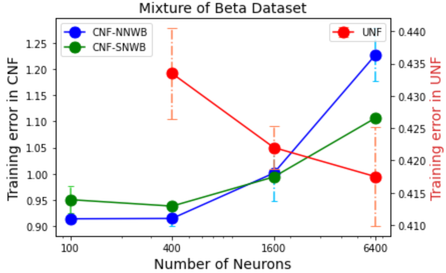
In Sec. 3, we theoretically show that overparameterized neural networks in CNFs can not approximate the target function in the bounded time steps or in the bounded change in weights, and in Sec. 4, we show that highly overparameterized neural networks provably learn target distribution. We now give empirical evidence of these claims. In Fig. 1, we plot training error after a fixed number of training iterations for a different amount of over-parameterization for both CNF and UNF models on a mixture-of-Gaussian and a mixture-of-Beta distribution datasets. The left and right -axes represent training error in CNF and UNF models, respectively. CNF-SNWB and CNF-NNWB denote CNF models with standard normal and normalized normal initialization of parameters, resp. We see that as we increase overparameterization in CNF models, training error becomes larger after a fixed number of training iterations, which means that larger CNF models need larger number of training iterations to learn the target function. But in UNFs, by increasing overparameterization, training error becomes smaller, which means that larger UNF models need smaller number of training iterations to learn the target function. Thus, our experimental results suggest that overparameterization in CNFs makes training slower and overparameterization in UNFs makes training faster. These experiments were done for a fixed learning rate. Similar patterns were observed for various different settings of learning rates except when training becomes unstable in CNFs. Since results in supervised learning also suggest that overparameterization makes training faster Neyshabur et al. 2015, our results on CNF are novel and surprising. Results on CNFs as well as results on UNFs on additional synthetic and real datasets, deeper models, various initializations, different learning rates and full experimental setup are given in Appendix I.
6 Conclusions and Limitaions
We gave the first end-to-end theoretical analysis of normalizing flows. We introduced the dichotomy between CNFs and UNFs: overparametrization seems to be hurting training of CNFs but for UNFs overparametrization does not hurt and we can analyze UNFs when the underlying network has one hidden-layer. We also proposed NF variants with desirable properties and these may find use in future work.
The main limitations of our work are the following which also suggests the main open problems: (1) A clear theoretical and empirical understanding of the role of overparameterization in CNFs remains an interesting open direction. As shown by our negative theoretical results, it seems necessary to analyze CNFs in the moderately overparametrized setting. However, this setting is not well-understood even in the supervised case. (2) For UNFs our analysis requires the overparametrized setting. (3) For the analysis we distill NF architectures to essentials—while this permits us to zero in on the main phenomena the more practical architectures are far more elaborate and performant and pose new theoretical challenges. (4) Our work assumes the autoregressive structure of the flow models. However, the role of overparameterized neural networks in other normalizing flow models such as coupling flows, residual flows, and other generative models such as VAEs is not well understood. (5) Our theoretical results have a one-hidden layer flow model but invertible flow models can be sequentially composed to construct an invertible map and in practice, flows models are sequentially composed to learn flexible target distributions. Extending our theoretical results for such models is an open problem.
References
- Jacot et al. [2018] Arthur Jacot, Clément Hongler, and Franck Gabriel. Neural tangent kernel: Convergence and generalization in neural networks. In Samy Bengio, Hanna M. Wallach, Hugo Larochelle, Kristen Grauman, Nicolò Cesa-Bianchi, and Roman Garnett, editors, Advances in Neural Information Processing Systems 31: Annual Conference on Neural Information Processing Systems 2018, NeurIPS 2018, 3-8 December 2018, Montréal, Canada, pages 8580–8589, 2018. URL http://papers.nips.cc/paper/8076-neural-tangent-kernel-convergence-and-generalization-in-neural-networks.
- Du et al. [2018] Simon S Du, Xiyu Zhai, Barnabas Poczos, and Aarti Singh. Gradient descent provably optimizes over-parameterized neural networks. In Proceedings of the 35th International Conference on Learning Representations, 2018. URL https://arxiv.org/abs/1810.02054.
- Allen-Zhu et al. [2019] Zeyuan Allen-Zhu, Yuanzhi Li, and Yingyu Liang. Learning and generalization in overparameterized neural networks, going beyond two layers. In Advances in neural information processing systems, pages 6158–6169, 2019.
- Zou et al. [2020] Difan Zou, Yuan Cao, Dongruo Zhou, and Quanquan Gu. Gradient descent optimizes over-parameterized deep relu networks. Machine Learning, 109:1–26, 03 2020. doi: 10.1007/s10994-019-05839-6.
- Arora et al. [2019] Sanjeev Arora, Simon S. Du, Wei Hu, Zhiyuan Li, and Ruosong Wang. Fine-grained analysis of optimization and generalization for overparameterized two-layer neural networks. In Kamalika Chaudhuri and Ruslan Salakhutdinov, editors, Proceedings of the 36th International Conference on Machine Learning, ICML 2019, 9-15 June 2019, Long Beach, California, USA, volume 97 of Proceedings of Machine Learning Research, pages 322–332. PMLR, 2019. URL http://proceedings.mlr.press/v97/arora19a.html.
- Goodfellow et al. [2014] Ian J. Goodfellow, Jean Pouget-Abadie, Mehdi Mirza, Bing Xu, David Warde-Farley, Sherjil Ozair, Aaron C. Courville, and Yoshua Bengio. Generative adversarial nets. In Zoubin Ghahramani, Max Welling, Corinna Cortes, Neil D. Lawrence, and Kilian Q. Weinberger, editors, Advances in Neural Information Processing Systems 27: Annual Conference on Neural Information Processing Systems 2014, December 8-13 2014, Montreal, Quebec, Canada, pages 2672–2680, 2014. URL http://papers.nips.cc/paper/5423-generative-adversarial-nets.
- Kingma and Welling [2014] Diederik P. Kingma and Max Welling. Auto-encoding variational bayes. In Yoshua Bengio and Yann LeCun, editors, 2nd International Conference on Learning Representations, ICLR 2014, Banff, AB, Canada, April 14-16, 2014, Conference Track Proceedings, 2014. URL http://arxiv.org/abs/1312.6114.
- Rezende and Mohamed [2015] Danilo Rezende and Shakir Mohamed. Variational inference with normalizing flows. volume 37 of Proceedings of Machine Learning Research, pages 1530–1538, Lille, France, 07–09 Jul 2015. PMLR. URL http://proceedings.mlr.press/v37/rezende15.html.
- Bowman et al. [2016] Samuel R. Bowman, Luke Vilnis, Oriol Vinyals, Andrew Dai, Rafal Jozefowicz, and Samy Bengio. Generating sentences from a continuous space. In Proceedings of The 20th SIGNLL Conference on Computational Natural Language Learning, pages 10–21, Berlin, Germany, August 2016. Association for Computational Linguistics. doi: 10.18653/v1/K16-1002. URL https://www.aclweb.org/anthology/K16-1002.
- Salimans et al. [2016] Tim Salimans, Ian Goodfellow, Wojciech Zaremba, Vicki Cheung, Alec Radford, Xi Chen, and Xi Chen. Improved techniques for training gans. In Advances in Neural Information Processing Systems, pages 2234–2242. 2016. URL http://papers.nips.cc/paper/6125-improved-techniques-for-training-gans.pdf.
- Arora et al. [2018] Sanjeev Arora, Andrej Risteski, and Yi Zhang. Do GANs learn the distribution? some theory and empirics. In International Conference on Learning Representations, 2018. URL https://openreview.net/forum?id=BJehNfW0-.
- Lucic et al. [2018] Mario Lucic, Karol Kurach, Marcin Michalski, Olivier Bousquet, and Sylvain Gelly. Are gans created equal? a large-scale study. In Proceedings of the 32nd International Conference on Neural Information Processing Systems, NIPS’18, page 698–707, 2018.
- Kobyzev et al. [2020] I. Kobyzev, S. Prince, and M. Brubaker. Normalizing flows: An introduction and review of current methods. IEEE Transactions on Pattern Analysis and Machine Intelligence, 2020.
- Papamakarios et al. [2019] George Papamakarios, Eric T. Nalisnick, Danilo Jimenez Rezende, Shakir Mohamed, and Balaji Lakshminarayanan. Normalizing flows for probabilistic modeling and inference. ArXiv, abs/1912.02762, 2019.
- Buhai et al. [2020] Rares-Darius Buhai, Andrej Risteski, Yoni Halpern, and David Sontag. Empirical study of benefits of overparameterization in single-layer latent variable generative models. In Proceedings of the 37th International Conference on Machine Learning, 2020. URL https://proceedings.icml.cc/static/paper_files/icml/2020/5645-Paper.pdf.
- Kong and Chaudhuri [2020] Zhifeng Kong and Kamalika Chaudhuri. The expressive power of a class of normalizing flow models. volume 108 of Proceedings of Machine Learning Research, pages 3599–3609, Online, 26–28 Aug 2020. PMLR. URL http://proceedings.mlr.press/v108/kong20a.html.
- Koehler et al. [2020] Frederic Koehler, Viraj Mehta, and Andrej Risteski. Representational aspects of depth and conditioning in normalizing flows. arXiv preprint arXiv:2010.01155, 2020.
- Lee et al. [2021] Holden Lee, Chirag Pabbaraju, Anish Sevekari, and Andrej Risteski. Universal approximation for log-concave distributions using well-conditioned normalizing flows, 2021.
- Santambrogio [2015] Filippo Santambrogio. Optimal Transport for Applied Mathematicians. Calculus of Variations, PDEs and Modeling. Birkhäuser, 2015.
- Huang et al. [2018] Chin-Wei Huang, David Krueger, Alexandre Lacoste, and Aaron C. Courville. Neural autoregressive flows. In Jennifer G. Dy and Andreas Krause, editors, Proceedings of the 35th International Conference on Machine Learning, ICML 2018, volume 80 of Proceedings of Machine Learning Research, pages 2083–2092. PMLR, 2018. URL http://proceedings.mlr.press/v80/huang18d.html.
- Cao et al. [2019a] Nicola De Cao, Wilker Aziz, and Ivan Titov. Block neural autoregressive flow. In Proceedings of the Thirty-Fifth Conference on Uncertainty in Artificial Intelligence, UAI 2019, Tel Aviv, Israel, July 22-25, 2019, page 511. AUAI Press, 2019a. URL http://auai.org/uai2019/proceedings/papers/511.pdf.
- Wehenkel and Louppe [2019] Antoine Wehenkel and Gilles Louppe. Unconstrained monotonic neural networks. In Hanna M. Wallach, Hugo Larochelle, Alina Beygelzimer, Florence d’Alché-Buc, Emily B. Fox, and Roman Garnett, editors, Advances in Neural Information Processing Systems 32: Annual Conference on Neural Information Processing Systems 2019, NeurIPS 2019, 8-14 December 2019, Vancouver, BC, Canada, pages 1543–1553, 2019. URL http://papers.nips.cc/paper/8433-unconstrained-monotonic-neural-networks.
- Neyshabur et al. [2015] Behnam Neyshabur, Ryota Tomioka, and Nathan Srebro. In search of the real inductive bias: On the role of implicit regularization in deep learning. In ICLR (Workshop), 2015.
- Cao et al. [2019b] Nicola De Cao, Wilker Aziz, and Ivan Titov. Block neural autoregressive flow. In Amir Globerson and Ricardo Silva, editors, Proceedings of the Thirty-Fifth Conference on Uncertainty in Artificial Intelligence, UAI 2019, Tel Aviv, Israel, July 22-25, 2019, page 511. AUAI Press, 2019b. URL http://auai.org/uai2019/proceedings/papers/511.pdf.
- Yehudai and Shamir [2019] Gilad Yehudai and Ohad Shamir. On the power and limitations of random features for understanding neural networks. In Advances in Neural Information Processing Systems, pages 6598–6608, 2019.
- Shalev-Shwartz and Ben-David [2014] Shai Shalev-Shwartz and Shai Ben-David. Understanding machine learning: From theory to algorithms. Cambridge university press, 2014.
- Nagarajan and Kolter [2019] Vaishnavh Nagarajan and J Zico Kolter. Generalization in deep networks: The role of distance from initialization. arXiv preprint arXiv:1901.01672, 2019.
- Dua and Graff [2017] Dheeru Dua and Casey Graff. UCI machine learning repository, 2017. URL http://archive.ics.uci.edu/ml.
- van den Berg et al. [2018] Rianne van den Berg, Leonard Hasenclever, Jakub Tomczak, and Max Welling. Sylvester normalizing flows for variational inference. In proceedings of the Conference on Uncertainty in Artificial Intelligence (UAI), 2018.
- Tomczak and Welling [2016] Jakub M Tomczak and Max Welling. Improving variational auto-encoders using householder flow. arXiv preprint arXiv:1611.09630, 2016.
- Papamakarios et al. [2017] George Papamakarios, Theo Pavlakou, and Iain Murray. Masked autoregressive flow for density estimation. In Proceedings of the 31st International Conference on Neural Information Processing Systems, NIPS’17, page 2335–2344, 2017. ISBN 9781510860964.
- Teshima et al. [2020] Takeshi Teshima, I. Ishikawa, Koichi Tojo, Kenta Oono, M. Ikeda, and M. Sugiyama. Coupling-based invertible neural networks are universal diffeomorphism approximators. ArXiv, abs/2006.11469, 2020.
- Lei et al. [2020] Qi Lei, Jason D. Lee, Alexandros G. Dimakis, and Constantinos Daskalakis. SGD learns one-layer networks in WGANs. In In Proceedings of the 37th International COnference on Machine Learning, 2020. URL https://proceedings.icml.cc/static/paper_files/icml/2020/4998-Paper.pdf.
- Balaji et al. [2021] Yogesh Balaji, Mohammadmahdi Sajedi, Neha Mukund Kalibhat, Mucong Ding, Dominik Stöger, Mahdi Soltanolkotabi, and Soheil Feizi. Understanding over-parameterization in generative adversarial networks. In International Conference on Learning Representations, 2021. URL https://openreview.net/forum?id=C3qvk5IQIJY.
- Li and Dou [2020] Yuanzhi Li and Zehao Dou. Making method of moments great again? – how can GANs learn the target distribution, 2020. URL https://arxiv.org/abs/2003.04033.
- Nguyen et al. [2019a] Thanh V. Nguyen, Raymond K. W. Wong, and Chinmay Hegde. On the dynamics of gradient descent for autoencoders. In The 22nd International Conference on Artificial Intelligence and Statistics, AISTATS 2019, 16-18 April 2019, Naha, Okinawa, Japan, volume 89 of Proceedings of Machine Learning Research, pages 2858–2867. PMLR, 2019a. URL http://proceedings.mlr.press/v89/nguyen19a.html.
- Nguyen et al. [2019b] Thanh V. Nguyen, Raymond K. W. Wong, and Chinmay Hegde. Benefits of jointly training autoencoders: An improved neural tangent kernel analysis. CoRR, abs/1911.11983, 2019b. URL http://arxiv.org/abs/1911.11983.
- Radhakrishnan et al. [2020] Adityanarayanan Radhakrishnan, Mikhail Belkin, and Caroline Uhler. Overparameterized neural networks can implement associative memory, 2020. URL https://arxiv.org/abs/1909.12362.
- Wainwright [2019] Martin J. Wainwright. High-Dimensional Statistics: A Non-Asymptotic Viewpoint. Cambridge Series in Statistical and Probabilistic Mathematics. Cambridge University Press, 2019. doi: 10.1017/9781108627771.
- Romberg [2012] Justin Romberg. Maximum of a sequence of gaussian random variables. 2012. URL http://cnx.org/contents/8bd316d8-6442-4f5a-a597-aef1d6202f87@1.
- Li and Yeh [2013] Yuan-Chuan Li and Cheh-Chih Yeh. Some equivalent forms of bernoulli’s inequality: A survey. Applied Mathematics, 4(07):1070, 2013.
- Maurer [2016] Andreas Maurer. A vector-contraction inequality for rademacher complexities. In International Conference on Algorithmic Learning Theory, pages 3–17. Springer, 2016.
Supplementary Material:
Learning and Generalization in Overparameterized Normalizing Flows
Appendix A Outline
In this section, we give outline of details and proofs of supplementary. We define common notations between Constrained Normalizing Flows results and Unconstrained Normalizing Flow results in Appendix B. Our results on CNFs from Section 3 from the main paper are discussed in detail in Theorem H.5 (Section H.1) and Theorem H.6 (Section H.2) and their proofs.
We give details about our result on UNFs (in Section 4) in Theorem G.6 and its proof (Section G). Our analysis begins with showing that if change in weights and biases from the initialization is small for a neural network, then training dynamics of the pseudo-network (linear approximation of neural network) is close to training dynamics of the neural network in Section D. In Section E, we show that with high probability there exist a pseudo-network which can approximate the derivative of target function. In Section F, we show that optimization problem for the pseudo-network is convex; therefore, combining results from Section E and Section D will give us the result that the loss of UNFs on the training data is close to the loss of target function. In section G, we prove generalization guarantees to test datasets and complete the proof of Theorem H.5.
Appendix B Notations
In this section, we define commonly used notations. We denote as a concatenation of 2 vectors and . For any 2 vectors and , denotes element wise multiplication of and vector. We use , and to denote , and norm of vector . For any matrix , we denote matrix norm as
where denotes row vector of matrix . We denote vector . Big- and Big- notation to hide only constants. We use to denote natural logarithm. For any constant , is denoted by set . We use to denote Gaussian distribution with mean and variance . We use to denote the indicator of the event . We say a function is -Lipschitz continuous if for all .
Appendix C Preliminaries
Recall that is the random variable corresponding to the data distribution and is a random variable with standard Gaussian or multivariate exponential distribution. There seems to be no well-accepted definition of standard exponential distribution; for our purposes the following natural defintion will serve well. The density of the standard exponential distribution at is given by when all , and by , otherwise. Let flow be an monotonic autoregressive function. Then standard change of density formula using invertibility of gives
To make an monotonic autoregressive function, we force function to be monotonic with respect to for any fixed where is dimension of . Recall that represents the vector including first elements of vector for any .
Unlike the constrained case where we model using a neural network, in unconstrained case we model derivative of function using neural networks. In normalizing flow, for all , we model using a neural network . To be specific,
We denote as . Here, is the +1 function given by for all . we use a one-hidden-layer neural network in , which is given by
We construct such that . We can reconstruct by integration:
The lower limit in our integral is because by our assumption on the support of the data distribution. Note that to reconstruct from the Jacobian, we need to evaluate the integrals. While this cannot be done exactly, good approximation can be obtained via numerical integration (also known as quadrature). We estimate via the general quadrature formula by
Here, is the number of quadrature points and the are the corresponding coefficients. We use simple rectangle quadrature, which arises in Riemann integration, and uses only positive coefficients with and . The loss function for normalizing flows is given by
Using standard exponential distribution as a base distribution, we get
| (C.1) |
where
For our theoretical result, we consider target functions whose derivative are given by
where , for all and are smooth functions with Taylor expansion and are positive integers. Our target function class is rich: the argument of is two-layer neural network with smooth activations.
We need to quantify the complexity of the functions: more complex functions allow representing more distributions but are also harder to learn. We begin by defining the complexity of univariate smooth functions used in the definition of target functions. Let have Taylor expansion , then its complexity for is given by which is a weighted norm of the Taylor coefficients. For example, when is one of , it is known that Allen-Zhu et al. 2019. Very roughly, captures how many samples are needed to learn up to error . For in our target class, complexity is defined to be .
For each neural network , we define its pseudo-network by , where
Note that our definition of pseudo-network is not the straightforward generalization from the supervised case: is not a linear approximation of because we are not taking linear approximation of final activation .
Appendix D Coupling
In this section, we will establish closeness between training dynamics of neural networks and pseudo network, which we will call as coupling. First, we will establish the coupling between and (Lemma D.4). Using coupling between and , we prove coupling between and (Lemma D.5). We also prove coupling between gradient and in Lemma D.7, which will be used in proving global optimization of neural network in Section F.
We define as
| (D.1) |
which will be used later in the proof of coupling between and . The upper bound on is useful to bound derivative of w.r.t. . We get the following upper bound on :
| (D.2) |
Define as
| (D.3) |
for any fixed constant .
Recall that loss function in case of CNFs is given by
Lemma D.1.
(Bound on change in weights) For every , for all , for any positive constant and for every with , with at least probability over random initialization, bound on change in weights after steps with learning rate is given by
Proof.
Lemma D.2.
(Bound on the number of changes in activation patterns) For every and for all , suppose and . Then, for every such that , with probability at least over random initialization, the number of activation patterns that change is at most . In other words, for at most fraction of , we have
for any positive constant .
Proof.
Define
| (D.7) |
The set contains indices of neurons for which indicator function doesn’t change its value if change in weights is bounded by . For every such that and for all , . For all , we have
| (D.8) |
Now, we need to bound the size of . We know that for all with , is Gaussian with and . Using Lemma K.5, we get
Using Fact K.7 (Hoeffding’s inequality) for (where for any positive constant , we get
which gives
∎
Lemma D.3.
(Bound on the difference between and ) For every , for all with and for every time step , with probability at least over random initialization, for any positive constants , we have
Proof.
Using 1-Lipschitz continuity of , we get
We bound :
| (D.9) |
where inequality (i) uses Lemma K.4 to upper bound with probability at least . ∎
Lemma D.4.
(Final bound on the difference between and ) For every , for all with and for every time step , with probability at least over the random initialization, and some positive constants and , we have
| (D.10) |
Proof.
We denote the upper bound as :
Lemma D.5.
(Coupling of the loss functions) For every , for all with and for every time step , with probability at least over the random initialization, loss function of neural network and pseudo-network are close for some positive constant and :
Using eq. (C.1), with probability at least over the random initialization, we have
Proof.
where inequality (i) follows from 1-Lipschitz continuity of with respect to . Inequality (ii) uses Lemma D.3. Using the definition of , with at least probability , we get
∎
Lemma D.6.
(Coupling of the gradients of functions) For every , for all with and for every time step , with probability at least over random initialization, gradient of derivative of neural network function and derivative of pseudo-network function with respect to parameters are close for any positive constant
Proof.
Lemma D.7.
(Coupling of the gradient of loss) For every , for all with and for every time step , with probability at least over random initialization, gradient of loss function with neural network and loss function with pseudo-network are close for some positive constant and :
Proof.
We define as
Note that is an upper bound on .
Appendix E Approximation
In this section, we will prove that each pseudo network can approximate any target function from target class with small offset from the weights of initialization. We first prove that expectation of multiplication of a fixed function and can approximate any smooth activation in target function (Lemma E.6). This is used to prove that can approximate any target function in target class in norm. Using Lipschitz continuity with respect to , we prove that is close to , where is any target function in the target class.
To prove results in this section, we require a number of new techniques on top of techniques from Allen-Zhu et al. 2019. The target functions in Allen-Zhu et al. 2019 are more restricted because norm of weights in target function is equal to 1 (i.e., ). In our paper, we relax this condition and allow any weights with their norm bounded by 1 (i.e., ). Our proof can easily be extended to weights bounded by any constant. Additionally, our proof requires to bound approximation error between pseudo network and target network, which is a stronger condition than approximation error given in Allen-Zhu et al. 2019, and requires a new proof technique.
Lemma E.1.
For any fixed constant and even , for any and , we have
Similarly, for any fixed constant and odd , for any and , we have
Proof.
Using summation formula from Fact K.1, we have
Expanding using multiplication formula of Hermite polynomial from Fact K.1, we get
| (E.1) |
Using Fact K.2, for even , we have
| (E.2) |
and for odd ,
| (E.3) |
Using Eq. (E.1), Eq. (E.2) and Eq.(E.3), we get
Using in the expectation, we have
| (E.4) |
Define as
Now, we divide our proof in two parts. In (a), we complete the proof for even and in (b), we do it for odd .
- (a)
- (b)
∎
Lemma E.2.
Define as
and define and as
For any , we have
| (E.7) | ||||
| (E.8) |
Proof.
The lemma follows from Lemma A.7 of Allen-Zhu et al. 2019. ∎
We will use two different view of the randomness. Define as and where and are standard normal random variables and is any positive constant. In alternative view of randomness, we write as
where . Define and where and are normal random variables with mean and variance. Using definitions of and , we get
where and are standard normal random variable.
Lemma E.3.
For every integer , there exists a constant with such that
Proof.
First, we will prove for even . By Lemma E.1, we get
| (E.9) |
where
Now, we try to bound the coefficient . Define as
For and for all odd with ,
Using above relation, we get
and
Using Eq.(E), we get
This completes the proof for even . Similarly for odd , using Lemma E.1, we get
| (E.10) |
where
Now, we will try to bound . Define as
For and for all even with , we get
Using above relation, we get
and
Using the formula of in Eq. (E), we have
This completes the proof for odd . ∎
Lemma E.4.
For any constant and for any arbitary function , we have
where , coefficient of taylor series of function,
Proof.
Using Taylor expansion of function , we get
where above relation follows from Lemma E.3 and is given by
∎
Lemma E.5.
For any and any positive integer , setting , we have
- 1.
- 2.
- 3.
The Lemma is same as Claim C.2 of Allen-Zhu et al. 2019.
Lemma E.6.
For any positive integer , for any , for every function , every , every with and , there exist a function such that
| (E.11) |
Proof.
Define . From Lemma E.4, we get
where
Using Lemma E.5, we have . Define as
Using definition of , we get
Using Lemma E.5, we have
This proves that for every function , every , every constant and for every , there exist a function such that we have
| (E.12) |
We denote for as orthogonal vectors of with . Now, using projection of on , we get
| (E.13) |
where for any such that is a normal random variable with 0 mean and variance. Define as . Similarly, define for . Now, dot product can be written as
| (E.14) |
where last inequality follows from . Here and are standard normal random variables. Setting and using Eq.(E.12), Eq. (E.13) and Eq.(E), we get
∎
Lemma E.7.
For all , for any , for any derivative of target function and for any with , there exist a set of parameters such that we have
Moreover, norm of is given by
Proof.
We denote pseudo network with parameters as:
Similarly, is given by . We will use function to approximate a neuron of target function for all . Setting and as
we get
Bounding , we get
∎
Define upper bound on as
Lemma E.8.
For any , for any , for any derivative of target function , for any and for any with , there exist a set of parameters such that, with atleast probability, we have
Proof.
We divide into five parts as
| (E.15) |
We know that the first part from Lemma E.7. Since , the second term . Using Lemma D.2 and Lemma D.3 for bounding the third term III, we get
| (E.16) |
We will use technique from Yehudai and Shamir 2019 to bound the fourth term IV. Define a function as
We will now bound the expectation of using McDiarmid’s inequality (Fact K.13). For every , we get
where last inequality follows with atleast probability by applying Lemma K.4 on and . Define as
Using Lemma 26.2 from Shalev-Shwartz and Ben-David 2014, we get
where are independent Rademacher random variables. Using Lipschitz continuity of ReLU activation, we get
Using Lemma 26.10 from Shalev-Shwartz and Ben-David 2014, we get
For , we have and therefore, we get
Using McDiarmid’s inequality (Fact K.13), we get
For , with at least probability, for all with , we have
| (E.17) |
To bound V, by Eq. (D), we know
| (E.18) |
where inequality follows from Eq. (D) with atleast probability and inequality follows from Lemma D.2 with atleast . Using Lemma E.7, Eq.(E), Eq.(E), Eq.(E.17) and Eq.(E), with atleast probability, we get
∎
Lemma E.9.
For any , for any target function , for any and for any with , there exist a set of parameters such that, with atleast probability, we get
Proof.
Using definition of , we get
where inequality follows from 1-Lipschitz continuity of and . The upper bound on is given by
∎
We define upper bound on as :
Appendix F Optimization
This section shows that SGD on the loss of the neural network can be closely approximated by the SGD on the loss of the pseudo-network (Theorem F.3). Since the loss function of the pseudo-network is convex in its parameters (Lemma F.1), we get global optimization of the pseudo network, and hence, global optimization of the neural network. Moreover, there exist a pseudo-network which can approximation the target function and achieve training loss close to the trainign loss of the target function (Section E). Therefore, SGD on the loss of the neural network can achieve training loss comparable to training loss of the target function (Theorem F.3).
First, we will start with proving convexity of the loss function of the pseudo-network.
Lemma F.1.
(Convexity of the loss function of the pseudo-network) The loss function of the pseudo-network is convex with respect to the parameters of the neural network, and therefore, loss satisfies first order condition of convexity for all and for all with :
Proof.
We decompose the loss function of the pseudo-network for each dimension into two parts:
where
We prove convexity of both and . We can write as
Note that is convex in and is linear in . As composition of any convex and linear function is convex, is convex. The first part of loss function is convex in because sum of convex functions is also convex. By writing in parts, we get
Using last equality in the above equation, we can see that is convex in and we know that is linear in . Therefore, is convex in because composition of any convex and linear function is a convex function. As and are convex, is also convex in because sum of convex functions is a convex function. ∎
Remark F.2.
When we use the standard Gaussian for the base distribution, then the loss function will be:
Note that the second term in the decomposition is convex with same argument given in Lemma F.1 and the first term is given by
Using the same argument given in Lemma F.1, we get that is convex in but each summand in is square of convex function, which may not be convex in . Therefore, can be non-convex in .
Recall that average loss of function on training set is defined as :
Similarly, average loss for and average loss for is denoted by and , respectively.
Theorem F.3.
(SGD achieves near-optimal loss) For every , for every learning rate and number of steps such that, with at least probability, we get
Proof.
Recall that is a pseudo network which approximates the target function . From Lemma F.1, we know that is convex in parameters , which gives
| (F.1) |
Recall that SGD update at time is given by
Using SGD update at time , We have
By taking expectation wrt , we get
| (F.2) |
Putting value of from Eq.(F.2) to (F), we get
By (D.3), (D.4) and (D), with atleast probability, we have
Averaging from to , we get
| (F.3) |
where last inequality follows with atleast . Recall that was defined in (D.18). The last equality also uses the fact that initial change in weights is equal to . Using Lemmas D.5 and E.9 respectively, with probability at least we have
We now choose values of and :
| (F.4) | ||||
where we use chosen value of to get upper bound on . Using above inequalities, we get the following equalities:
Using Lemma E.9, we get
To get value of , we will first upper bound , and :
Multiplication of and will be
Taking as
| (F.5) |
we get
Using (D.10), we get
| (F.6) |
Using given choice of from (F.5), we get
Similarly, using given choice of from (F.5), we get
Using Eq.(F.4) and Eq.(F.5), with at least probability, we get
Taking and rescaling as , with at least probability, we get
To find the lower bound on probability, we use :
where inequality follows from for all . To find lower bound on , we use same inequality:
where last inequality follows from given choice (Eq. (F.5)) of sufficiently high . Now, we will lower bound quantity:
where last inequality follows from the value of . Finally, we can say that, with at least probability, we get
∎
Appendix G Generalization
In this section, we prove generalization guarantees to complement our optimization result, and complete the proof of our main theorem (Theorem G.6) about efficiently learning distributions using univariate normalizing flows. Recall that denotes an empirical average of over training data and denotes expectation with respect to underlying data distribution. The proof in this section can be broadly divided two parts. First, we prove that empirical average and are close to expectation and , respectively (Lemma G.3 and Lemma G.4). Second, we prove that and are close to and , respectively (Theorem G.6).
Recall that the approximate loss function is given by
where
Similarly, we define for the target function .
Lemma G.1.
(Empirical Rademacher complexity for two-layer neural network) For every constant , for any number of training samples , for any time , with probability at least over random initialization, the empirical Rademacher complexity is bounded by
where denotes first dimension of training example.
Proof.
Using part (a) of Lemma K.16, we get that has Rademacher complexity . Using part (b) of Lemma K.16, we get that has Rademacher complexity . Using part (c) of Lemma K.16, we get that class of functions in has Rademacher complexity
where inequality (i) follows from Lemma K.4 with at least probability over random initialization.
∎
We denote and as maximum and minimum value of :
We find upper bound on maximum and lower bound on minimum value of the loss for the target function in terms of and :
and define them respectively as and :
| (G.1) | ||||
Lemma G.2.
(Small value of neural network at initialization) For any dimension , for any constant and , with probability at least , we have
Proof.
Suppose, for any given , there are indicators with value 1. Without loss of generality, we can assume that indicators from to is 1. Then,
Now, applying Hoeffding’s inequality (Fact K.8) on any dimension for the sum in first part of the above equation, with atleast probability, we get
| (G.2) |
Using union bound, we get
Using definition of norm, we have
Plugging in above equation, with probability at least , we have
and using relation between and norm, we have
| (G.3) |
Similarly, using Hoeffding’s inequality (Fact K.8), with at least probability, we get
Plugging , with at least probability, we get
| (G.4) |
Using Eq.(G.3) and Eq.(G.4), with probability at least , we have
| (G.5) | ||||
This completes the proof. ∎
Lemma G.3.
For any constant , for any dimension , any time , any , suppose that the number of samples satisfies
| (G.6) |
Then, with at least probability over random initialization, the population loss of any functions of the set is close to the empirical loss, i.e.
Proof.
We know that the loss for dimension depends on neural network through vector. Using Fact K.17, with at least probability, we get
| (G.7) |
where . In the above equation, constant denotes upper bound on the loss and denote standard Lipschitz constant of with respect to . We denote as coordinate-wise Lipschitz continuity of loss function as following:
Using Lemma K.6, standard Lipschitz constant of is given by
| (G.8) |
To get constant (i.e., upper bound on ), we use Lipschitz property of . We construct such that .
| (G.9) |
Note that depends upon vector and similarly, depends upon . Finding upper bound for all with , we get
where inequality follows from Lemma G.2, Lemma K.4 and Eq.(D.6). The inequality uses our choices of and from Eq.(F.4). We define as upper bound on :
| (G.10) |
Using value of and Eq.(G), we get upper bound on :
Using value of in Eq.(G.7) and Lemma G.1, with at least probability, we get
By summing over all dimension , with atleast probability, we get
Using and our choice of given in (G.6), with probability at least , we have
∎
Lemma G.4.
(Concentration on approximated loss of target function) Suppose is sufficiently high such that it satisfies
If satisfies above condition, then with at least probability, population loss of target function is close to empirical loss i.e.
Proof.
Using Hoeffding’s inequality (Fact K.8), we have
Taking as
with at least probability , we get
| (G.11) |
∎
Corollary G.5.
Before stating our main theorem, we recall and define necessary terms used in stating the theorem. Recall that
Recall that for any function with Taylor expansion , then its complexity for any is given by
which is a weighted norm of the Taylor coefficients. Recall that we define upper bound on complexity of learning any function as
Now, we will state our main theorem.
Theorem G.6.
(loss function is close to optimal) For every , for every and , for any target function with finite second order derivative and number of quadrature points and number of training points , with at least probability, we have
where is given by
Proof.
First, we will try to bound for all with :
Similarly, bounding error for for all with , we will get
To get , we will use Eq.(G.10).
where inequality (i) follows by plugging in Eq.(G), with . Define as upper bound on ,
Taking as
| (G.12) |
Using given value of , we get that
| (G.13) | ||||
| (G.14) |
Using these relations, we get
By the definition of KL divergence, we get
∎
Appendix H Problem in Training of Constrained Normalizing Flow
In this section, we provide details of why different initializations cause problems (described in section 3) in the training of Constrained Normalizing Flows. Recall that the loss function of normalizing flow with Gaussian distribution as base distribution is given by
where function is parameterized using neural networks . The dimension of the function . The neural network in CNF is defined as
Here, is a small constant and is a normalization constant which only depends on . We use to denote parameters of and to denote parameters of all neural networks. Initial weights and are sampled from half-normal distribution with parameters and , resp. The half-normal random variable with parameters is given by simply where . Here denote the Gaussian distribution with mean and variance . Other weights ( for ) are sampled from . We optimize the objective using projected SGD. Note that in this case, the constraints are very simple and projected SGD incurs very little overhead.
The pseudo network function is given by , where is given by
with constraints for all . We decompose pseudo network in two parts:
where and is given by
The loss function for pseudo network is given b
where . The pseudo network , which approximates the neural network , will be
with constraints , for all . We decompose into two parts: , where
Note that only depends upon initialization and does not depend on parameters .
Let denote the target function and denote some complexity measure of . We devide our analysis into two cases based on variance of and . (1) In the first case, standard deviation satisfies . (2) In the second case, standard deviation satisfies . We call the first case larger variance initalization case and the second one smaller variance intialization case. Analysis for larger variance case is given in Section H.2 and analysis for smaller variance case is given in Section H.1.
H.1 Problem in optimization for smaller variance initialization case
In this section, we will provide details about the problem in smaller variance initialization case for Constrained Normalizing Flows (CNFs). We prove in Theorem H.5 that if we choose small learning rate and number of time steps according to the theorem statement, then function learned by sufficiently overparameterized CNFs is close to a linear function. To prove the theorem, we start by bounding maximum possible change in weights and biases during iterations in Lemma H.1. Using bound on change in weights, we establish closeness between function value given by neural networks and function value given by pseudo networks (Lemma H.3). We, then, prove that for any , pseudo network at time is close to a linear function (Lemma H.4). Using closeness between neural network and pseudo network and linearity of pseudo network, we get that neural networks are close to a linear function for given small learning rate and number of time steps . Note that choosing similar values of and in supervised learning enables the provable successful training of neural network. The same issue in approximation arises for all activations with continuous derivative.
Recall that neural network is given by
and derivative is given by
We denote as .
Lemma H.1.
(Bound on change in weights and biases) For every with , every and time step , upper bound on weights and biases is given by following with at least probability for any constant , .
Proof.
We first find upper bound on the derivative of loss function and and . We denote . By taking derivative of with respect to , we get
We assume that is -lipschitz continuous wrt and -lipschitz continuous wrt . Assuming and , we have
Assuming , we get
Using Lemma K.4 for and , with probability at least , we have
| (H.1) |
For projected gradient descent, we get
By defining and as
we get
| (H.2) | ||||
In general, for any , we can write
By taking , we get
Note that is sum of an arithmetic-geometric progression (AGP). Using Fact K.14, we can simplify the above sum as
| (H.4) |
Using Eq.(H.1) to bound in Eq. (H.2), we get
This completes the proof of upper bounding . We use a similar procedure for . By taking derivative , we get
We assume that is -lipschitz wrt and -lipschitz wrt . Additionaly, using and , we get
Using Lemma K.4 for and , with probability at least , we get
| (H.5) |
For projected gradient descent, summing from time step to , we get
Using Eq.(H.1), we get
This completes the proof. ∎
Define and as upper bound on and :
Lemma H.2.
For any , target function with some complexity measure , any which satisfy , any hidden layer size , any learning rate and , with at least probability, we get
Proof.
To simplify expression of , we will use Fact K.12. First, we will check the condition for Fact K.12:
Choosing sufficiently high such that , we get
By choosing sufficiently high , the condition of Fact K.12 satisfies. Now, simplifying expression of using Fact K.12, we get
Simplifying expression of in simillar manner as , we get
∎
Lemma H.3.
(Coupling between neural network and pseudo network) For every with , every and every time step , with probability at least over random initialization, we have
Proof.
Bounding difference between and , we get
for some . Using and , we get
Using Lemma K.4 and using , with at least probability, we have
Using union bound for all , we complete the proof. ∎
Lemma H.4.
For any , every and every time step , any target function with some complexity measure of target function , any variance with , any hidden layer size , choosing learning rate and , with probability at least over random initialization, we get
Proof.
Recalling the definition of :
Subtracting the linear function from will give us the following:
| (H.6) |
First, we will try to find upper bound on :
where inequality follows from 1-Lipschitz continuity of function. Using Lemma K.4 on and , with probability at least , we get that
Using above inequality in Eq. (H.1), with probability at least over random initialization, we get
Using Lemma K.4 and Lemma H.1, with probability at least , we get
Using bound on and from Lemma H.2, we get
Using and re-scaling by , we get
Using for , we get
∎
Theorem H.5.
For any , any , any target function with some complexity measure of target function , any which satisfy , any hidden layer size , choosing normalization constant such that , learning rate and , with probability at least 0.9 over random initialization, Projected SGD on neural network after iterations
| (H.7) |
where and are given by
H.2 Problem in optimization for larger variance initialization case
In this section, we will provide details about the problem for larger variance initialization case. Recall that only depends upon initialization and does not depend on . Hence, it can not approximate the target function after the training, therefore needs to approximate target function with subtracted but in this case, we prove in Theorem H.6 that if norm of change in weights is small then is very small for sufficiently large ; therefore, it can not approximate every target function. We also provide reasons and details in Lemma H.7 about the requirement of small norm of change in weights . In short, small norm of change in weights is required to maintain coupling between neural networks and pseudo networks. For large variance initialization case, we have
Theorem H.6.
(small value of ) For any standard deviation , for any , any constant and any , , if upper bound on norm of change of parameters is given by
then for all with , with probabillity at least , we have
Given upper bound on is necessary to ensure closeness between neural network and pseudo network (More details given in Lemma H.7).
Proof.
Using the definition of , we get
where inequality follows from Lemma K.4 with at least probability. Using upper bound on from the theorem statement, with at least probability, we get
This completes the proof. ∎
Recall that we denote derivative as . Similarly, we use to derivative of .
Lemma H.7.
(Requirement of having small -norm of change in weights ) For any constant , for all , if following bound either on holds,
then, with at least probability, coupling between and can be lost. More precisely,
Proof.
First, we will find upper bound on difference between and :
where inequality follows from Lemma K.4 with probability at least . Using bounds on norm , we get
Using union bound on all , with probability atleast , for all , we get
Taking and , with atleast 0.98 probability, for all , we get
∎
Appendix I Additional experiments
In this section, we show experimental results for both CNF and UNF on different datasets. First, we describe experimental setup in Subsection I.1. Then, we discuss our main observations for constrained normalizing flow and unconstrained normalizing flow in Subsection I.2 and I.3. In Subsection I.5, we plot training curves for both CNF and UNF for different learning rates and datasets. Codes for the experiments are available at https://github.com/kulinshah98/overparam-NFs.
I.1 Experimental Setup
Datasets.
We use five synthetic datasets for our experiments. All datasets contain 10,000 data points. The details about the datasets are given below:
- •
Mixture of Gaussian Dataset: Data in this dataset lies in 1D and is generated from mixture of 2 Gaussians with means at 2.5 and -2.5. The standard deviation of both Gaussians is 1.
- •
Mixture of Beta Dataset: Data in this dataset lies in 1D and is generated from mixture of 3 Beta distribution. The parameters of Beta distributions are given by (5, 30), (30, 5) and (30, 30).
- •
Grid Dataset: Data in this dataset lies in 2D. Figure of the data is given in 2. Brightness at any point in this 2D plot represents the unnormalized probability density of that point.

Figure 2: Grid dataset - •
5D Mixture of Gaussian dataset: Data in this dataset lies in 5D and is generated from mixture of 10 Gaussians.
Architecture.
We use similar architecture as described in Section 3 and Section 4 for both constrained and unconstrained normalizing flows. In all our experiments, we fix the weights of the output layer and train the weights and biases of the hidden layer. In UNFs, we use one-hidden layer network for all datasets while in CNFs, we use one-hidden layer network for 1D datasets and use two-hidden layer network for Grid dataset and three-hidden layer network for 5D Mixture of Gaussian dataset. We initialize weights of neural network as described in Section 3 and Section 4. We choose (standard deviation of top layer of neural networks in both UNF and CNF) from using the training error after a fixed number of iteration as a metric to evaluate.
Training Procedure.
We use same training procedure for both constrained and unconstrained normalizing flows as described in Section 3 and Section 4. We use same base distribution as used in theoretical results for both CNF and UNF (i.e., standard Gaussian for CNFs and standard exponential for UNFs). Although, we believe that our experimental result can hold for all common distributions as a base distribution. In all our experiments, we use mini-batch SGD with batch size 32 for the training.
All our results are averaged over 5 different iterations. We used NVIDIA Tesla P100 GPU for approx 1000 hours to generate our final experimental results. Our experimental results validate the dichotomy between constrained and unconstrained normalizing flows which was established in Section 3 and Section 4.
I.2 Results for constrained normalizing flow
In Section 3, we suggested that high overparameterization may adversely affect training for constrained normalizing flows . In this section, we give empirical evidence for our claims. We use Gaussian distribution as a base distribution in all our experiments of constrained normalizing flow. We experiment with two different initialization for weights and biases of the hidden layer. 1) Gaussian distribution with zero-mean and variance () where is number of neurons in hidden layer. We call CNF with this initialization as CNF-NNWB (CNF with Normalized Normal initialization for Weights and Biases) and 2) Standard Gaussian distribution (). We denote CNF with this initialization as CNF-SNWB (CNF with Standard Normal initialization for Weights and Biases). We observe training error and distance of parameters from initialization after a fixed number of iterations for both CNF-NNWB and CNF-SNWB. We made following two observations:
Effect of overparameterization on training speed of CNF.
In Figure 3 and Figure 4, we plot width of neural networks versus training error after a fixed number of iterations and for a fixed learning rate. We see that training error for CNF models increases as we increase overparameterization of neural networks, which means that to reach a fixed training error, larger models take more number of training updates. This shows that for any fixed learning rate, as we increase overparameterization in CNF, training speed decreases. This phenomenon is consistent across different datasets, different learning rates and different initializations. This result is novel and surprising because in supervised learning, overparameterization helps in faster convergence for a fixed learning rate Neyshabur et al. 2015 and we are not aware of any other settings where overparametrization has such strong negative effect.
|
|
 |
 |
 |
 |
 |
 |
Effect of overparameterization on distance of parameters from initialization.
Figure 5 has plots of width of neural networks versus distance of parameters from the initialization after a fixed number of training iterations. From the figure, we see that as we increase overparameterization in CNF models, distance from the initialization also increases. From our previous observation, we know that after a fixed number of training iterations, training error increases as overparameterization increases. Combining experiment on distance with our previous observation, we get that to achieve same training error, more overparameterized model have larger distance compared to their smaller counterparts. This result is surprising because in supervised learning, it is known that more overparameterized model have smaller distance of parameters from the initialization Nagarajan and Kolter 2019.
 |
 |
 |
 |
 |
 |
I.3 Results for unconstrained normalizing flow
In Section 4, we prove that overparameterized neural network can efficiently learn the data distribution. In this section, we will provide empirical evidence that overparameterization helps in training of UNF. Similar to CNF, we study training error and distance of parameters from initialization after a fixed number of training iterations. We made following two observations:
Effect of overparameterization on training speed of UNF.
In Figure 3, we see that training error after a fixed number of iterations decreases with increasing width of neural networks in UNF, which means that to reach a fixed training error, larger models need smaller number of training updates. This implies that for any fixed learning rate, increasing overparameterization in UNF increases training speed. This trend is consistent with supervised learning, where it is known that overparameterization helps in faster convergence for a fixed learning rate Neyshabur et al. 2015.
Effect of overparameterization on distance of parameters from initialization.
Figure 5 shows that as we increase overparameterization in UNF models, distance of parameters from the initialization decreases. Our previous observation was that after a fixed number of training iterations, training error decreases or remains almost same as overparameterization increases. Combining our observation on distance with our previous observation, we get that to achieve a fixed training error, more overparameterized model require smaller distance compared to their less overparameterized counterparts. This result is consistent with supervised learning, where it is known that more overparameterized model have smaller distance of parameters from the initialization Nagarajan and Kolter 2019.
I.4 Results on Miniboone dataset
To show experimental results on a real-world dataset, we use miniboone dataset [Dua and Graff 2017]. The dataset contains examples of electron neutrino and muon neutrino. This dataset contains around 30K examples and lies in 43 dimensions. To test our phenomenon, we modify the official implementation of block neural autoregressive flow (BNAF) [Cao et al. 2019b] for CNF and Unconstrained Monotonic Neural Network Flow [Wehenkel and Louppe 2019] for UNF. We use 3 hidden layers for CNF and 3 hidden layers for both embedding network and derivative network. We use one flow model for both of them and use a mini-batch SGD optimizer with a learning rate of 0.001. The figure to illustrate the change in training error by changing the width of the network for each dimension is plotted in 6. From the figure, we see that the training error for CNFs increases with an increase in width of the network whereas the training error for UNFs decreases with an increase in width of the network. This observation supports our theoretical results.

 |
 |
 |
 |
 |
 |
I.5 Training curves for Constrained and Unconstrained Normalizing Flow
To provide a complete picture, we provide training error and distance of weights and biases from the initialization for all time step during the training. We first discuss results for CNFs and then move our discussion to UNFs.
Constrained Normalizing Flow.
In Figure 8, 9, 11, 10, 12 and 13, we plot number of epochs on x-axis and y-axis can be training error, distance of weights or distance of biases from the initialization.
In all figures, we see that for any fixed learning rate, curve of training error for smaller is always below than curve of training for larger , which proves our claim that increasing overparameterization hurts the training speed of CNF models. This phenomenon is consistent for all datasets, different initializations and various learning rates. Only exception to this phenomenon is results on mixture of Gaussian dataset for and and learning rate equal to 0.025 but note that in this case, the training of CNF for is very unstable and therefore, at some time steps, curve has slightly smaller training error than because of unstable training.
Apart from training error, we see that distance for biases (that is, norm of ) is always larger for large . The difference is clearly visible and significant in comparison figures of large hidden layer nodes ( and ). This is consistent across different initializations, datasets and learning rates. Only exception to this trend is results on mixture of Gaussian dataset for and . Even in this case, distance is comparable for and .
 |
 |
 |
 |
 |
 |
 |
 |
 |
 |
 |
 |
 |
 |
 |
 |
 |
 |
 |
 |
 |
 |
 |
 |
 |
 |
 |
 |
 |
 |
 |
 |
 |
 |
 |
 |
 |
 |
 |
 |
 |
 |
 |
 |
 |
 |
 |
 |
Unconstrained Normalizing Flow.
Similar to Constrained Normalizing Flows, we study the effect of overparameterization on convergence speed and -norm of and . The first row of Figure 14 contains results for mixture of Gaussians dataset and the second row contains results for mixtures of beta distributions dataset. From the first column of Fig. 14, we see that the training speed for larger is better or comparable to smaller . Additionally, we see that -norm of and decreases significantly with increasing . This results validate our theoretical finding that distance of parameters from the initialization decreases with increasing .
|
|
|
|
|
|
Appendix J Related Work
Previous work on normalizing flows has studied different variants such as planar and radial flows in Rezende and Mohamed 2015, Sylvester flow in van den Berg et al. 2018, Householder flow in Tomczak and Welling 2016, masked autoregressive flow in Papamakarios et al. 2017. Most variants of normalizing flows are specific to certain applications, and the expressive power (i.e., which base and data distributions they can map between) and complexity of normalizing flow models have been studied recently, e.g. Kong and Chaudhuri 2020 and Teshima et al. 2020. Invertible transformations defined by monotonic neural networks can be combined into autoregressive flows that are universal density approximators of continuous probability distributions; see Masked Autoregressive Flows (MAF) Papamakarios et al. 2017, UNMM-MAF by Wehenkel and Louppe 2019, Neural Autoregressive Flows (NAF) by Huang et al. 2018, Block Neural Autoregressive Flow (B-NAF) by Cao et al. 2019a. Unconstrained Monotonic Neural Network (UMNN) models proposed by Wehenkel and Louppe 2019 are particularly relevant to the technical part of our paper.
Koehler et al. 2020 theoretically study representation ability of affine couplings (a type of normalizing flow) and particularly analyze several aspects such as depth of normalizing flows. Lei et al. 2020, Balaji et al. 2021 show that when the generator is a two-layer tanh, sigmoid or leaky ReLU network, Wasserstein GAN trained with stochastic gradient descent-ascent converges to a global solution with polynomial time and sample complexity. Using the moments method and a learning algorithm motivated by tensor decomposition, Li and Dou 2020 show that GANs can efficiently learn a large class of distributions including those generated by two-layer networks. Nguyen et al. 2019a show that two-layer autoencoders with ReLU or threshold activations can be trained with normalized gradient descent over the reconstruction loss to provably learn the parameters of any generative bilinear model (e.g., mixture of Gaussians, sparse coding model). Nguyen et al. 2019b extend the work of Du et al. 2018 on supervised learning mentioned earlier to study weakly-trained (i.e., only encoder is trained) and jointly-trained (i.e., both encoder and decoder are trained) two-layer autoencoders, and show joint training requires less overparameterization and converges to a global optimum. The effect of overparameterization in unsupervised learning has also been of recent interest. Buhai et al. 2020 do an empirical study to show that across a variety of latent variable models and training algorithms, overparameterization can significantly increase the number of recovered ground truth latent variables. Radhakrishnan et al. 2020 show that overparameterized autoencoders and sequence encoders essentially implement associative memory by storing training samples as attractors in a dynamical system.
Appendix K Useful facts
Fact K.1.
For any , let denote the degree probabilists’ Hermite polynomial
The Hermite polynomials satisfy following summation and multiplication formulas.
Fact K.2.
Let denote the degree probabilists’ Hermite polynomial, then for , we have
Lemma K.3.
Suppose and is chi-squared distribution with following property for all .
Proof.
From example 2.11 from Wainwright 2019, for and is chi-squared distribution with following property for all .
Using above equation for ,
∎
Lemma K.4.
Let be independent random variables from , then with at least probability, following holds.
Proof.
Lemma K.5.
For standard Gaussian random variable from , the following anti-concentration inequality holds:
Proof.
(From Du et al. 2018) For the standard Gaussian random variable ,
Using , we get the required result. ∎
Lemma K.6.
Suppose function is -Lipschitz continuous and -coordinate wise Lipschitz continuous i.e.
If a function satisfies -coordinate wise Lipschitz continuity for all , then function follows following inequality.
Moreover, the function also satisfies standard Lipschitz continuity with Lipschitz constant where inequality between and is as follows.
Proof.
Define and .
where last inequality follows from Cauchy-Schwarz inequality. ∎
Fact K.7.
(Hoeffding’s inequality on Binomial random variable) If we have a binomial random variable with parameters (total number of trials) and (probability of success). For , following inequality holds.
Fact K.8.
(Hoeffding’s inequality) Let be independent random variables where is bounded in the interval . Then, for any , we have
Fact K.9.
(Half-normal distribution) If follows a normal distribution with with mean 0 and variance , , then follows a half-normal distribution with mean .
Fact K.10.
For a gaussian random variable , , we have
Fact K.11.
The sum of reciprocals of the squares of the natural numbers is given by
Fact K.12.
(Theorem of Li and Yeh 2013) For any and ,
Fact K.13.
(McDiarmid’s Inequality) Let be some set and let be a function such that for some , for all and for all , we have
Let are independent random variables taking values in . Then,
Fact K.14.
If Arithmetic-Geometric Progression(AGP) is as follows.
where is the initial term, is the common difference and is the common ratio. The sum of the first terms of the AGP () is given by
Definition K.15.
Let be a set of functions and be a finite set of samples. The empirical Rademacher complexity of with respect to is defined by
The following results are standard and can be found, e.g., in Allen-Zhu et al. 2019.
Lemma K.16.
Rademacher complexity has the following properties:
- a.
For any and with . The function class has Rademacher complexity .
- b.
Given classes functions, .
- c.
Given classes of functions of type and suppose is a fixed vector, then satisfies where is a 1-Lipschitz continuous function.
Proof.
These are standard results and can be found in Allen-Zhu et al. 2019 and Shalev-Shwartz and Ben-David 2014. ∎
Fact K.17.
(Rademacher Complexity) If are classes of functions of type and is a -Lipschitz-continuous function for every in the support of , then
where is set of functions obtained by composing with , that is . Using vector contraction inequality from Maurer 2016, we get