Cooperative Evasion by Translating Targets with Variable Speeds
Abstract
We consider a problem of cooperative evasion between a single pursuer and multiple evaders in which the evaders are constrained to move in the positive direction. The evaders are slower than the vehicle and can choose their speeds from a bounded interval. The pursuer aims to intercept all evaders in a given sequence by executing a Manhattan pursuit strategy of moving parallel to the axis, followed by moving parallel to the axis. The aim of the evaders is to cooperatively pick their individual speeds so that the total time to intercept all evaders is maximized. We first obtain conditions under which evaders should cooperate in order to maximize the total time to intercept as opposed to each moving greedily to optimize its own intercept time. Then, we propose and analyze an algorithm that assigns evasive strategies to the evaders in two iterations as opposed to performing an exponential search over the choice of evader speeds. We also characterize a fundamental limit on the total time taken by the pursuer to capture all evaders when the number of evaders is large. Finally, we provide numerical comparisons against random sampling heuristics.
I Introduction
We consider a single pursuer multi-evader pursuit evasion problem in which the aim of the pursuer is to intercept all of the evaders in a fixed given sequence. The evaders are constrained to move along the positive direction. The pursuer follows the Manhattan distance, i.e., moving parallel to the -axis followed by moving parallel to the -axis. The aim of the evaders is to cooperatively maximize the total time to intercept all evaders. Such a set-up arises in riot control or border protection scenarios in which a ground or air vehicle would like to optimally visit mobile locations headed toward a boundary/asset, or in UAV monitoring of vehicles along a highway. This setup is also applicable in multiple robotic decoy deployment [1].
I-A Related work
Since the seminal work by Isaacs in [2], much has been done in the field of pursuit evasion with a lot of focus on multi-agent pursuit evasion [3, 4, 5]. The case of a single pursuer and 2 evaders has been extensively analyzed [6], [7]. Protector-Prey-Predator [8] and Target-Attacker-Defender differential game [9] are some examples of this scenario. With more than two evaders, the complexity of the problem grows exponentially with number of evaders. The problem of successive pursuit with cooperative multiple evaders is considered in [10, 11, 12] and [13]. Our problem differs from [14, 15] as the pursuer follows a fixed strategy and the evaders are constrained to move in a fixed direction and can choose their individual speeds from a bounded interval to maximize the total intercept time. Thus, the evasive strategies are based on the range of evader speeds.
I-B Contributions
We consider an optimal evasion problem between a single pursuer and evaders. The pursuer moves with unit speed. The evaders are constrained to move in the positive direction such that their speeds , lie in the interval with . The evaders need to choose their speeds in order to maximize the total intercept time. We first present a complete solution to the optimal evasion problem for . We then show, for general , that the optimal choice of the speed for each evader is one of the extremes, i.e., or . We further show that, by enforcing cooperation among evaders, they are able to maximize the total intercept time. In order to implement the cooperative strategies, it is important to determine the conditions under which cooperation is optimal. Such conditions are also provided in this paper. We present an algorithm which assigns the evasive strategies to the evaders in two iterations as opposed to performing an exponential search over the choice of evader speeds. For sufficiently large , for which the global optimum is difficult to compute, we establish a fundamental upper bound to the total intercept time taken by the pursuer to capture all evaders. Finally, we provide comparisons through numerical results.
I-C Organization
The paper is organized as follows. Section II comprises the formal problem definition. In section III, we derive an evasive strategy for multiple evaders and provide a Sequential-Greedy-Cooperation algorithm. Section IV establishes a fundamental upper bound on the total time to intercept all evaders. Section V presents the numerical simulations. Finally, section VI summarizes this paper and outlines directions for future work.
II Problem formulation
We consider an optimal evasion problem played between a single pursuer with simple motion and mobile evaders. We denote the pursuer as and evaders as with . The pursuer with initial location at is assumed to be moving with unit speed either along the or the axis. We term this pursuit strategy as Manhattan pursuit, and is formally defined as follows.
Definition 1 (Simple Manhattan pursuit)
Given initial locations and of an evader and the pursuer respectively, the pursuer
- 1.
moves with unit speed along the positive or negative direction until and then,
- 2.
moves with unit speed along positive or negative axis to intercept the evader.
The evaders, initially located at , are constrained to move along the positive direction with simple motion such that their instantaneous speeds , , lie in the interval with (Fig. 1). The pursuer is said to the target when its location coincides with that of the target. The game when the pursuer intercepts the last evader. A strategy for an evader is a measurable function, defined as , where the notation denotes the set of all locations .
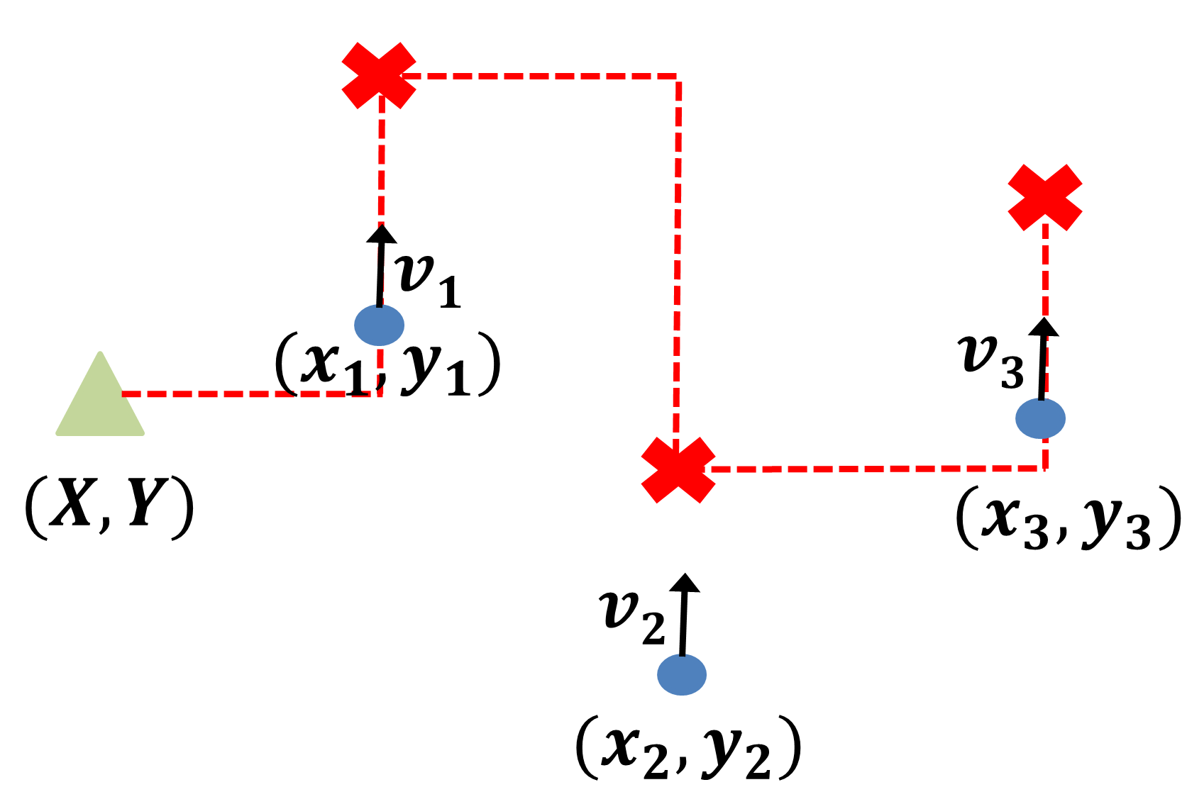
The goal is to solve the following problem.
Problem II.1 (Optimal evasion)
Given that the pursuer follows a fixed order to intercept the evaders, determine strategies for the evaders that maximizes the total time taken by the pursuer to intercept all evaders.
III Evasive Strategy
We begin with the case of a single evader followed by two evaders, and then present the more general case. We start by defining the following simple Manhattan pursuit strategy.
III-A Single Evader
In this section, we first consider the case of a single evader and a pursuer, located at and respectively. We first present a result on the time taken to intercept a single evader. This will be used in deriving the optimal strategy for the evader. We denote , where and as the time taken by the pursuer to intercept evader moving with speed after intercepting evader . Specifically, is the time taken to intercept the first evader moving with speed . For brevity, we omit the proofs for the single evader case as they can be derived by following the steps in the proof of the general case presented later.
Lemma III.1 (Time to intercept a single evader)
The time taken by to intercept is
Lemma III.2 (Monotonicity of time to intercept)
The time is a monotonically increasing function of if . Otherwise, is a monotonically decreasing function of .
Remark 1
The time to intercept is monotonic even when the pursuer follows a Euclidean strategy, i.e., given the initial locations of and , as and respectively, the vehicle moves towards , where is
Lemma III.2 characterizes the monotonic nature of . This only means that the maximum is achieved at one of the extremes. The next theorem characterizes the evader’s optimal choice of speed.
Theorem III.3 (Single evader optimal strategy)
Given the initial locations and of the evader and the pursuer respectively, the optimal strategy for the evader is
Proof.
We provide only an outline. We find a location such that , where (resp. ) is the time to intercept when evader moves with (resp. ). From Lemma III.1, . This means that if , then from Lemma III.2, it would not matter if the evader moves with or as , and will be maximum at both and . If , then, from Lemma III.2, either or . Assuming and thus, by contradiction, we get the result. The second case is analogous and we get the result. ∎
We now consider the case of two evaders and derive the optimal evasion strategies for both evaders. We say that an evader moves greedy if it moves with speed that maximizes its own intercept time. An evader cooperates if it moves with a speed that maximizes the total intercept time. We denote the greedy strategy of evader as and the cooperative strategy as .
III-B Two evaders
Similar to previous section, we first derive an expression for the time taken to intercept the evaders followed by the optimal strategy for both evaders.
Let the first evader be located at and move with speed and the second evader be located at and move with speed . Then, the following result summarizes the time to intercept after intercepting . For ease of reference, we introduce the following condition:
| (1) |
Lemma III.4 (Time to intercept )
The time taken by to intercept after intercepting is
Proof.
Consider the case when condition (1) holds, after the intercept of . This means that after the completion of stage (1) for the pursuit of , the evader’s -coordinate strictly exceeds . The additional time to intercept the second evader is
Thus, total time to intercept after intercepting is
The second case can be derived analogously and this concludes the proof. ∎
Lemma III.5 (Monotonicity of time to intercept )
Given that moves with , the time is monotonically increasing function of if condition (1) holds. Otherwise, is a monotonically decreasing function of .
We now characterize an optimal greedy strategy for . In what follows, we denote .
Lemma III.6 (’s greedy strategy)
The greedy strategy for for a greedy moving with is
Proof.
From Lemma III.5, is maximized at either or . The aim is to find the critical location such that if was located at , then the time = . Note that this is possible only if condition (1) holds for and does not hold for . From Lemma III.4, we get . This means that if , then irrespective of ’s choice of or , the time to intercept will be the same and from Lemma III.5, the time to intercept will be maximum at both and , given that moves greedy. Now, consider that the initial location of is such that . From Lemma III.5, the time to intercept will be maximized only at either or and so assume that is maximized at , i.e., . This implies . This is a contradiction as . This means that will be maximized if moves at . Similarly, when it can be shown that will be maximized if moves at and has been omitted for brevity. In the case when condition (1) does not hold for or holds for , then it implies that and respectively. This concludes the proof. ∎
Lemma III.6 yields a greedy strategy for when and both move greedily. However, it might be better for the evaders to cooperate to maximize the total intercept time. We now characterize the conditions on cooperation between the two evaders.

We define that a point , located at , is above point , located at , if and we define point is below point if .
Lemma III.7 (Conditions on cooperation)
Given the initial locations of , , and as , , and respectively, cooperates with if
(i) Case 1:
| (2) |
(ii) Case 2:
| (3) |
Proof.
Let the initial location of satisfy and initial location of satisfy . Then, from Theorem III.3, to maximize its own intercept time, , moves with . Also, from Lemma III.6, moves with in order to maximize its own intercept time . As the pursuer follows the Manhattan pursuit strategy, the time taken to cover the path in the y-direction to intercept and then is the same as the time taken to cover the path in y-direction to intercept only from the initial pursuer location (see Fig.2 (a)). Mathematically,
Thus, in order to increase the total time to intercept, and need to cooperate. One way to cooperate is that moves with a speed such that is intercepted below the pursuer, i.e., and moves greedily, i.e., with (see Fig 2 (b)). This is only possible if
If , then for any speed for , , and so the total distance covered in the y-direction to intercept and will be the same as the total distance covered in the y-direction to intercept , from the pursuer’s initial location , irrespective of ’s choice. The only other way in which and can cooperate in order to increase the total intercept time is when moves greedily, i.e., with and with speed such that such that intercept of is below the intercept location of (see Fig. 2 (c)). Thus, to determine which of the two scenarios yield the greater time to intercept, we arrive at a condition .
Note that as and are monotonic in and respectively, so the above condition is checked only at the extreme values, i.e., and . Thus, this means that should cooperate only if equation (2) holds. Furthermore, if the initial location of was such that , then from Lemma III.3, moves greedily, i.e., with speed . Since, this will already ensure that and so, there is no need for cooperation. Case 2 is analogous. This concludes our proof. ∎
Theorem III.8 (Optimal cooperative strategy for )
Given the initial locations , , and of , and , respectively, if the conditions for cooperation in Lemma III.7 hold, then the optimal cooperative strategy for evader is
Proof.
Consider that case 1 of Lemma III.7 holds. Then moves with speed such that . We know from Lemma III.7 that the conditions on cooperation ensure that the total time to intercept during cooperation is higher than the greedy choice. Since is monotonic in , from Lemma III.2, . The second case is derived analogously. This concludes the proof. ∎
In this subsection, we analyzed the case of 2 evaders, primarily to highlight the underlying problem structure. Next, we will consider the case of evaders. Similar to the two evader case, we will first present a result on the time taken to intercept the evader after intercepting the evader. Then we will present results on the greedy and cooperative strategies between and .
III-C Evaders
For ease of presentation, we will denote as for some and for brevity, we denote as . We present the following condition for ease of reference.
| (4) |
Lemma III.9 (Time to intercept )
The time taken by to intercept , moving with , after intercepting , moving with , is
Proof.
We establish this result using mathematical induction. Lemma III.4 yields the base of induction for . Assume that for some , the result holds. Consider that the initial location of the next evader, , is such that . This means that after the completion of stage (1) of simple pursuit of , the X-coordinate of the pursuer equals and at the same time, the evader’s y-coordinate strictly exceeds the pursuers y-coordinate . Thus, the time to intercept after intercepting will be
Thus, by induction the result holds for any value of . The other case is derived analogously. ∎
Lemma III.10 (Monotonicity of time to intercept)
Given that each , moves with , the time is monotonically increasing function of if condition (4) holds. Otherwise, is a monotonically decreasing function of .
Proof.
Since Lemma III.10 establishes that the time to intercept a evader is maximized at either or , finding an optimal strategy for all evaders would require analyzing all possibilities in the worst case.
We now present an algorithm that assigns respective strategies to the evaders in just two iterations.
The algorithm, summarized in Algorithm 1, first assigns the greedy strategies to all evaders. Then, it assigns cooperative strategies by considering two sequentially paired evaders at a time.
Now, we will present the results that the algorithm uses in assigning the strategies.
if and can cooperate, , then 1
Lemma III.11 (Evader k’s greedy strategy)
The greedy strategy for , when each , moves with is
Proof.
Suppose the result holds for some . Consider the next evader, . Similar to the proof of Lemma III.6, we find . If , then, from Lemma III.10, the time will be maximized at either or . Thus, assuming yields which is a contradiction and so . Moreover, by induction, the result holds for any value of . Case 2 is proved analogously. This concludes our proof. ∎
The previous lemma presented a result on the greedy strategy of any evader . This result is the first step of the Algorithm 1. As the second step of Algorithm 1 requires to check the conditions of cooperation between two consecutive evaders, we will now present a result on the conditions if two evaders should cooperate or not. We introduce the notation, .
Lemma III.12 (Cooperation conditions for )
Given the initial locations of , , and as , , and respectively, then will cooperate with if
(i) Case 1:
and
| (5) |
(ii) Case 2:
and
| (6) |
where determined by Algorithm 1.
Proof.
Let us assume that this result holds for some . The idea is to prove this result using induction by deriving the conditions for cooperation between and . For brevity, we will reuse Figure 2 with the two evaders and in the figure corresponding to and respectively. Suppose that the initial location of satisfies and the location of satisfies . Then, from Lemma III.11, moves with to maximize the component out of its intercept time and moves with to maximize . This implies that when completes stage 1 for the pursuit of , is below . As the pursuer follows the Manhattan pursuit strategy, the time taken to cover the path in the y-direction to intercept and then equals the time taken to cover the path in the y-direction to intercept only from the pursuer’s location (2 (a)). Note that the pursuer is located at the intercept location of . So, to increase the total time to intercept, and need to cooperate which can occur in only two ways.
The first is that moves with speed satisfying , which means that intercepts below the intercept point of and moves greedily, i.e., with (Fig. 2 (b)). This is possible only if holds. If , then for any speed for , the total distance covered in the -direction to intercept and will be the same as the total distance covered to intercept from the pursuer’s location, irrespective of ’s choice.
The second case in which and cooperate is if moves greedily with and moves with speed such that , i.e., the intercept location of is below the intercept location of (Fig. 2 (c)). To determine which of the two scenarios yield greater intercept time, we arrive at the condition
which yields the conclusion that should cooperate with only if equation (III.12) holds. This concludes our proof for case 1. Case 2 can be proved by following the steps for Case 1 and has been omitted for brevity. ∎
Lemma III.12 establishes the conditions for cooperation between any two consecutive evaders. The next result characterizes the cooperative strategies of the evaders.
Theorem III.13 (Cooperative strategy for )
If the conditions on cooperation in Lemma III.12 hold, then the optimal strategy for during cooperation with is
Proof.
Assume that the result holds for . The idea is to prove this result by induction by deriving this result for . Suppose case 1 from Lemma III.12 holds for and . From Lemma III.12, we know in order to cooperate with , moves with a speed such that , i.e., is intercepted below the pursuer’s location. We also know from the same lemma that these conditions on cooperation ensure that the total time to intercept while cooperation is higher than total time to intercept when the evaders move greedy. Now, since is monotonic in , . Similar steps can be followed for case 2. ∎
Remark 2 (Sandwiched evader)
For some , if Lemma III.12 holds for evader and as well as and , then evader moves greedy.
IV Fundamental Limit
In the previous sections, we considered that the pursuer followed a fixed strategy to capture all evaders. We now establish a fundamental upper bound, for a large number of evaders, on the total time taken to intercept all evaders by the pursuer following any strategy. We first provide some existing results that will be useful in establishing the bound.
Given a set of points, a Euclidean minimum Hamiltonian path (EMHP) is the shortest path through points such that each point is visited exactly once. When the points are translating with some constant speed , then the shortest tour though the points is called Translational minimum Hamiltonian path (TMHP) [16].
Lemma IV.1 (Length of EMHP tour)
Given points in a rectangle in the plane, where and , there exists a path that starts from a unit length edge of the rectangle, passes through each of the points exactly once, and terminates on the opposite unit length edge, with length upper bounded by
Proof.
The proof is similar to the proof provided in [17] for a rectangle and thus, has been omitted. ∎
To calculate the EMHP tour through translating points that move with speed , the points are scaled by defining a conversion map such that [16].
Lemma IV.2 (Length of TMHP tour [16])
Let the initial and final point be denoted as and respectively, and denote a constant speed of all evaders, then the length of the TMHP tour is where, denotes the length of the EMHP starting with point , moving through points and ending at point .
The optimal order followed by the vehicle in the TMHP solution is the same as the optimal order followed by the vehicle in the EMHP solution.
Denote as the total number of evaders that move with and as the total number of evaders that move with . Let and denote the area of the smallest enclosing rectangular environment that the and evaders occupy initially. We assume that all of the evaders are initially located within a rectangular environment of area . The pursuer’s strategy is to capture all the evaders first, followed by capturing all the evaders moving with . This is because if the pursuer captures the evaders first then naturally, the evaders moving with will be further away from the pursuer.
Let be the time taken by the vehicle to capture all of the evaders and be the time taken to intercept the last evader that moves with and the first evader that moves with after capturing all of the evaders respectively. Let be the total time taken by the vehicle to capture all of the remaining evaders. The next result characterizes an upper bound on the time taken by the pursuer to capture all evaders following any strategy.
Theorem IV.3 (Upper bound on intercept time)
Let and be the difference between the initial and -coordinate of the last evader captured moving with and the first evader that is captured moving with . Then, from Lemma IV.1 and Lemma IV.2, the total time taken by the pursuer to capture all evaders is where,
Moreover, for large , is maximum for
where denotes the integer nearest to .
Proof.
The outline of the proof is as follows. The expression for and follows directly from Lemma IV.1 and noting that is large. The expression for follows from [16]. Consider that the vehicle has just finished capturing all evaders. Then, all the evaders moving with would have translated in the direction. Note that the area will remain the same as it was initially. Since is large for large , the distance between the vehicle after capturing the last evader moving with and the first evader moving with will be large. Furthermore, since and is large, the pursuer will always be above all evaders moving with after capturing evaders and thus, we get the expression for . The evaders can select such that the total time is maximized. Mathematically, . If we relax the requirement of to be a real number then the function is concave with global maximum in the domain . This follows as . Thus, to find the maximizer, we use the first derivative test, i.e., and then find the closest integer value that maximizes . By taking the derivative of with respect to , we get , where,
In the worst case, the evader initial locations will cover the area completely, i.e., . Adding and equating to zero, and noting that is large, and yields
where . Since, , we get the result. Furthermore, since at the critical point , is indeed the point of maximum. This concludes the proof. ∎
V Simulation Results
We first present the numerical results for Algorithm 1.
We compare the mean of the total time to intercept all evaders using Algorithm 1 to the mean of the total time to intercept all evaders by randomly sampling over the evader speeds of either or (see Figure 3). For each value of , we randomly generate the initial locations of the evaders and the pursuer and we consider 50 Monte Carlo trials. To select the best evader speeds, we choose samples uniformly randomly over the set, which guarantees that the violation probability is less than a small quantity [18], where . We compute the maximum over the samples and then report the mean value in Figure 3. We observe that Algorithm 1 outperforms random sampling.
Figure 4 shows a comparison when is selected uniformly randomly to the upper bound obtained by for given initial locations. To obtain the EMHP tour required for the time to intercept evaders, the linkern11 1 The TSP solver linkern is freely available for academic research use at http://www.math.uwaterloo.ca/tsp/concorde/. solver was used. We consider 50 Monte Carlo trials for each value of and report the mean and standard deviation. It is observed that the total time to intercept all evaders by randomly selecting is well below the upper bound obtained from . Thus, by performing an additional optimization to select the evaders can reach the upper bound on time to intercept. This means that a strategy that only depends on may be sub-optimal for the evaders.


VI Conclusions and Future Work
An optimal evasion problem between single a pursuer and multiple evaders was addressed. It is shown that by enforcing cooperation among evaders, they are able to maximize the total interception time. Conditions where cooperation is optimal are also presented which are crucial to implement the cooperative strategies. An upper bound on the total time to intercept all evaders is also presented.
In subsequent work, a generalized setup of multiple pursuers and evaders will be considered. Constant factor approximations for both, the evaders and the pursuers will also be addressed. Identifying which evaders should move with is another possible extension.
References
- [1] R. Ragesh, A. Ratnoo, and D. Ghose, “Analysis of evader survivability enhancement by decoy deployment,” in 2014 American Control Conference. IEEE, 2014, pp. 4735–4740.
- [2] R. Isaacs, Differential games: a mathematical theory with applications to warfare and pursuit, control and optimization. Courier Corporation, 1999.
- [3] V. R. Makkapati and P. Tsiotras, “Optimal evading strategies and task allocation in multi-player pursuit–evasion problems,” Dynamic Games and Applications, vol. 9, no. 4, pp. 1168–1187, 2019.
- [4] A. R. Girard and P. T. Kabamba, “Proportional navigation: optimal homing and optimal evasion,” SIAM Review, vol. 57, no. 4, pp. 611–624, 2015.
- [5] J. Selvakumar and E. Bakolas, “Evasion from a group of pursuers with a prescribed target set for the evader,” in 2016 American Control Conference (ACC). IEEE, 2016, pp. 155–160.
- [6] Z. E. Fuchs, P. P. Khargonekar, and J. Evers, “Cooperative defense within a single-pursuer, two-evader pursuit evasion differential game,” in 49th IEEE Conference on Decision and Control (CDC). IEEE, 2010, pp. 3091–3097.
- [7] K. Zemskov and A. Pashkow, “Construction of optimal position strategies in a differential pursuit-evasion game with one pursuer and two evaders,” Journal of applied mathematics and mechanics, vol. 61, no. 3, pp. 391–399, 1997.
- [8] D. W. Oyler, P. T. Kabamba, and A. R. Girard, “Pursuit–evasion games in the presence of obstacles,” Automatica, vol. 65, pp. 1–11, 2016.
- [9] E. Garcia, D. W. Casbeer, K. Pham, and M. Pachter, “Cooperative aircraft defense from an attacking missile,” in 53rd IEEE Conference on Decision and Control. IEEE, 2014, pp. 2926–2931.
- [10] A. A. Chikrii and S. Kalashnikova, “Pursuit of a group of evaders by a single controlled object,” Cybernetics and Systems Analysis, vol. 23, no. 4, pp. 437–445, 1987.
- [11] I. Shevchenko, “Guaranteed approach with the farthest of the runaways,” Automation and Remote Control, vol. 69, no. 5, pp. 828–844, 2008.
- [12] A. Belousov, Y. I. Berdyshev, A. Chentsov, and A. Chikrii, “Solving the dynamic traveling salesman game problem,” Cybernetics and Systems Analysis, vol. 46, no. 5, pp. 718–723, 2010.
- [13] S.-Y. Liu, Z. Zhou, C. Tomlin, and K. Hedrick, “Evasion as a team against a faster pursuer,” in 2013 American Control Conference. IEEE, 2013, pp. 5368–5373.
- [14] W. L. Scott and N. E. Leonard, “Optimal evasive strategies for multiple interacting agents with motion constraints,” Automatica, vol. 94, pp. 26–34, 2018.
- [15] K. Krishnamoorthy, S. Darbha, P. P. Khargonekar, D. Casbeer, P. Chandler, and M. Pachter, “Optimal minimax pursuit evasion on a Manhattan grid,” in 2013 American Control Conference. IEEE, 2013, pp. 3421–3428.
- [16] M. Hammar and B. J. Nilsson, “Approximation results for kinetic variants of TSP,” in International Colloquium on Automata, Languages, and Programming. Springer, 1999, pp. 392–401.
- [17] S. D. Bopardikar, S. L. Smith, F. Bullo, and J. P. Hespanha, “Dynamic vehicle routing for translating demands: Stability analysis and receding-horizon policies,” IEEE Transactions on Automatic Control, vol. 55, no. 11, pp. 2554–2569, 2010.
- [18] T. Alamo, R. Tempo, and A. Luque, “On the sample complexity of randomized approaches to the analysis and design under uncertainty,” in Proceedings of the 2010 American Control Conference. IEEE, 2010, pp. 4671–4676.