Finding important edges in networks through local information

En-Yu Yu Affiliation: school of computer science and engineering
UESTC

943530714@qq.com Yan Fu Affiliation: school of computer science and engineering
UESTC
fuyan@uestc.edu.cn Jun-Lin Zhou Affiliation: school of computer science and engineering
UESTC
jlzhou@uestc.edu.cn Duan-Bing Chen* Affiliation: school of computer science and engineering
UESTC
Union Big Data Tech. Inc.
dbchen@uestc.edu.cn(Correspondence)

Abstract

In transportation, communication, social and other real complex networks, some critical edges act a pivotal part in controlling the flow of information and maintaining the integrity of the structure. Due to the importance of critical edges in theoretical studies and practical applications, the identification of critical edges gradually become a hot topic in current researches. Considering the overlap of communities in the neighborhood of edges, a novel and effective metric named subgraph overlap (SO) is proposed to quantifying the significance of edges. The experimental results show that SO outperforms all benchmarks in identifying critical edges which are crucial in maintaining the integrity of the structure and functions of networks.

Index Terms:

complex networks, critical edges, local information, robustness

I Introduction

With the acceleration of global informatization, human life is closely related to various complex networks[1, 2, 3, 4]. Electricity, water and gas networks affect people’s daily life[5]; road, railway and aviation networks affect people’s travel[6]; various popular social networks affect the spiritual life of individuals and the entire society[7]. In real networks, a few nodes and edges act pivotal roles and have great influence on the structure and functions of networks[8, 9, 10, 11]. Identifying critical nodes and edges has widely used in many applications such as analysis of cascading failures, control of infectious diseases and marketing of goods. In previous researches, the significance of nodes has been measured by numerous methods[12, 13, 14, 15, 16], yet how to evaluate the importance of edges receives less attention. In a complex network, the scale of edges is larger than that of nodes and the complexity of networks is often determined by edges. Therefore, the identification of critical edges is more difficult and meaningful[17, 18].

To identify critical edges, current methods mainly focus on the structural information of networks. Ball et al. [19] pointed out that the importance of an edge can be measured by the change of the average distance of the network after removing this edge. Similar to the betweenness centrality of nodes[20], Newman et al.[21] used the betweenness of edges (EB) to quantify the importance of edges. Yu et al.[22] proposed a method named $BCC_{MOD}$ , and it was significantly better than EB on all test networks. These algorithms based on global information have good results on small-scale networks, however, they are unsuitable for large-scale networks since they are time-consuming. Many researchers begin to use local information to characterize the significance of edges in order to reduce the time complexity. Holme et al.[17] supposed that edges between critical nodes are more important than other edges and proposed degree product (DP) index to evaluate the significance of edges. Consider the influence of node’s common neighbors on the importance of edges, topological overlap (TO) was proposed by Onnela et al.[23]. Cheng et al.[24] found that edges in a small clique with its endpoints in large cliques are important in connecting the network. Based on this idea, the bridgeness (BN) index was proposed. Liu et al.[25] proposed diffusion intensity (DI) to identify critical edges from the perspective of spreading dynamics. Besides, there are many other methods such as eigenvalues[26], link entropy[27] and nearest neighbor connections[28] to measure the importance of edges, which will not be introduced here.

In this paper, considering the overlap of communities in the neighborhood of edges, a novel and effective index named subgraph overlap (SO) is proposed. In SO index, the importance of an edge is characterized by the overlap of communities in its second-order neighborhood. In the experimental section, the performance of SO and five benchmark methods (DP, TO, DI, BN, SN) is measured by the robustness index[29]. The results on different networks show that SO is better than other methods in identifying critical edges which are crucial in maintaining the communication among different communities in networks. In addition, as a local index,SO is suitable for large-scale networks.

II Theory and Methods

II-A Network

Refer to caption — Fig. 1: Schematic diagram of static network: (a) undirected, unweighted; (b) directed, unweighted; (c) undirected, weighted; (d)directed, weighted.

A static network is usually expressed as $G=(V,E)$ , where $V=\{v_{1},v_{2},\dots,v_{N}\}$ is the node set and $E\subseteq V\times V$ is the edge set ( $|V|=N,|E|=M$ ). Usually, we use $e_{ij}$ to represent the edge connecting node $i$ and node $j$ . And the adjacency matrix $\mathrm{A}\in\mathbb{R}^{|V|\times|V|}$ is often used to calculate and store networks. The specific expression is as follows :

\mathrm{A}[v_{i},v_{j}]=a_{ij}=\begin{cases}0&\text{ if }(v_{i},v_{j})\notin E\\ 1&\text{ if }(v_{i},v_{j})\in E\end{cases}

(1)

As shown in Fig 1, static networks contain static undirected networks, static directed networks, static weighted networks, and static unweighted networks according to whether the edges have directions and weights. In this paper, we are using unweighted networks.

In a static network $G$ , The number of edges directly connected to node $i$ is often called the degree of node $i$ and expressed by $k_{i}$ . For detail, $k_{i}$ is defined as:

k_{i}=\sum_{j=1}^{N}a_{ij},

(2)

and nodes directly connected to node $i$ are called neighbors of node $i$ , denoted by $\Gamma_{i}$ . $\textlangle k\textrangle$ is the average degree of $G$ .

The distance between nodes is also one of the important structural parameters. In an static unweighted network, the path connecting node $i,j$ with the least edges is called the shortest path and the distance $d_{i,j}$ represents the number of edges included in it. In addition, the nodes whose distance to node $i$ is $l$ are called $l$ -hop neighbors of node $i$ .

II-B Subgraph Overlap Index

Previous studies[30, 31] pointed out that in facilitating communications among communities in the network, edges between two different communities in the network are often more important than those within communities. And edges between large communities are more important than other edges, and inversely proportional to other links between the two communities. At the same time, the method using global information is only can be used in small-scale networks due to the high time complexity, such as edge betweenness[21]. Inspired by above ideas, we tried to characterize the importance of edges by the overlap of communities in the neighborhood of edges. Then, a novel and effective index named subgraph overlap (SO) is proposed.

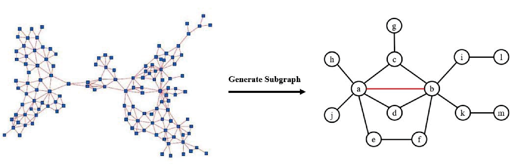
For a given static network $G$ and edge $e_{ij}$ , $G_{ij}$ is a subgraph of $G$ which contains node $i,j$ and nodes whose distance to $i$ or $j$ is no more than 2. The SO index is defined as :

SO(i,j)=\frac{max(1,|\Gamma_{i}^{(2)}\cap\Gamma_{j}^{(2)}|)^{2}}{|G_{ij}|},

(3)

where $|G_{ij}|$ represents the number of nodes in $G_{ij}$ . $\Gamma_{i}^{(2)}$ is the set of nodes whose distance to node $i$ is no more than 2 in $G_{ij}\setminus{e_{ij}}$ ( $\Gamma_{i}^{(2)}$ contains node $i$ ). Lower SO value indicates that the edge is more likely to connect large communities and there are few other connections between these two communities.

In addition, as shown in Fig 2(a) and (b), after removing $e_{ab}$ , if the community where node $a$ is located is no longer connected to the community where node $b$ is located ( $|\Gamma_{a}^{(2)}\cap\Gamma_{b}^{(2)}|=0$ ), the importance of $e_{ab}$ should be measured by the size of subgraph $G_{ab}$ , so the minimum value of the numerator is set to 1. The SO index only depends on local topological information and the time complexity is $O(M\textlangle k\textrangle^{2})$ .

A brief introduction to the calculation process of SO index is shown in Fig 3. In order to get $SO(a,b)$ , we first extract the subgraph $G_{ab}$ from the original network, obviously, $|G_{ab}|=13$ . Then we need to calculate $\Gamma_{a}^{(2)}$ and $\Gamma_{b}^{(2)}$ in $G_{ab}\setminus{e_{ab}}$ . In the subgraph $G_{ab}$ , $|\Gamma_{a}^{(2)}\cap\Gamma_{b}^{(2)}|=\{v_{a},v_{b},v_{c},v_{d},v_{e},v_{g},v_{f}\}$ , so $SO(a,b)=7^{2}/13=3.769$ .

II-C Benchmark Methods

In this paper, five well-known existing metrics such as topological overlap[23], degree product[17], diffusion intensity[25], bridgeness[24] and second-order neighborhood[32] are used to compare with SO. Same as SO, all benchmark methods use only local information.

Degree product (DP)[17]:

DP(i,j)=k_{i}k_{j}.

(4)

Topological overlap (TO)[23]:

TO(i,j)=\frac{|\Gamma_{i}\cap\Gamma_{j}|}{|\Gamma_{i}\cup\Gamma_{j}|-2},

(5)

where $\Gamma_{i}$ is the set of neighbors of node $i$ .

Diffusion intensity (DI)[25]:

DI(i,j)=\frac{(k_{i}-1)+(k_{j}-1)-2*|\Gamma_{i}\cap\Gamma_{j}|}{2}.

(6)

Bridgeness (BN)[24]:

BN(i,j)=\frac{\sqrt{|S_{i}||S_{j}|}}{|S_{ij}|},

(7)

where $S_{i}$ is the largest fully connected subgraph which contains node $i$ ( $S_{ij}$ contains $e_{ij}$ ).

Second-order neighborhood (SN)[32]:

SN(i,j)=\frac{|s_{i}^{(2)}\cap s_{j}^{(2)}|}{|s_{i}^{(2)}\cup s_{j}^{(2)}|},

(8)

where $s_{i}^{(2)}$ is the 2-hop neighbors of node $i$ in the subgraph $G\setminus{e_{ij}}$ .

III Experiments

III-A Datasets

In experiments, the data set contains one synthetic and eight real networks. (1) BA, a synthetic network generated by the scale free model[33]. (2) Citeseer, a citation network contains a selection of the CiteSeer dataset[34]. (3) Email, an email network at an university[35]. (4) Powergrid, a power network in the western America[5]. (5) Faa, an air traffic control network which is constructed from the USA’s FAA [36]. (6) Figeys, a protein network[37]. (7) Adjnoun, an adjacent words network of the novel David Copperfield[38]. (8) Sex, a sexual intercourse network[39]. (9) USair, an airport transportation network in US[36]. Some basic topology features of each network can be found in Table I.

TABLE I: The basic topology features.

\langle c\rangle

and

H

represent the average clustering coefficient and the degree heterogeneity, respectively.

Name	$N$	$M$	$\langle k\rangle$	$k_{max}$	$c$	$H$
BA	1000	4975	9.9500	112	0.0421	2.0808
Citeseer	3279	4552	2.7764	99	0.1435	2.4900
Email	1133	5451	9.6222	71	0.2201	1.9421
Powergrid	4941	6594	2.6690	19	0.0801	1.4503
Faa	1226	2408	3.9282	34	0.0675	1.8727
Figeys	2239	6432	5.7454	314	0.0399	9.7474
Adjnoun	112	425	7.5892	49	0.1728	1.8149
Sex	16730	39044	4.6675	305	0	6.0119
USair	1574	17215	21.8742	314	0.5042	5.1303

III-B Results

The performance of SO is evaluated by edge percolation process[40, 41]. For detail, remove edges from the network in turn according to the ranking results of each method, after removing the same proportion of edges, the greater the change in the network, the more important the removed edges. In this paper, the impact on the network connectivity after edges are removed is estimated by the famous measure named robustness $R$ [29] which is defined as

R=\frac{1}{M}\sum_{i=1}^{M}\sigma(i/M),

(9)

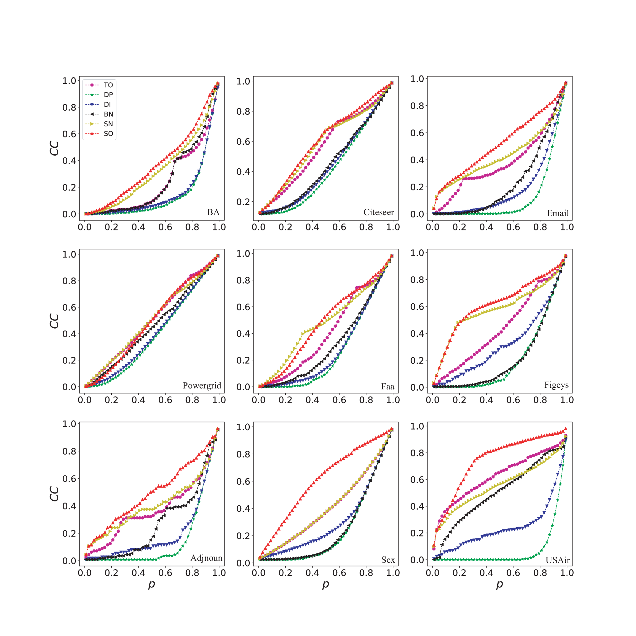
where $\sigma(i/M)$ indicates the ratio of nodes in the maximum connected component after removing edges with the ratio $i/M$ . Obviously, the method with smaller $R$ can decompose the network faster, which means that it can better rank the edge significance.

Fig 4 shows the process of network decomposition in nine networks. It can be seen that SO is the fastest of all methods to reduces $\sigma$ to 0.2 in all networks except Faa. In Faa, SO is the fastest of all methods to reduces $\sigma$ to 0.4. The robustness $R$ of SO and other benchmark methods are shown in Table II and it is easy to find SO has the best result for each network. All results show that decomposing the network according to the results of SO can destroy the robustness of the network the fastest. This also proves that the ranking results given by SO are more reasonable.

TABLE II: Comparison of

R

in all networks with highlighting the best results in bold.

Networks	TO	DP	DI	BN	SN	SO
BA	0.7419	0.8248	0.8143	0.7348	0.6633	0.6266
Citeseer	0.2041	0.2180	0.1968	0.1920	0.2062	0.1472
Email	0.5534	0.8092	0.7623	0.6410	0.5233	0.4691
Powergrid	0.2651	0.2417	0.2320	0.2159	0.2567	0.1691
Faa	0.5043	0.5636	0.5651	0.5238	0.4575	0.4454
Figeys	0.5376	0.6999	0.6495	0.6847	0.4054	0.3691
Adjnoun	0.6189	0.8005	0.7816	0.6655	0.5936	0.5114
Sex	0.5568	0.5984	0.5965	0.5889	0.5568	0.3430
USair	0.2851	0.8939	0.7244	0.3455	0.3342	0.2495

In addition to robustness $R$ , the impact on the network connectivity after edges are removed is also can be estimated by the average connectivity $\bar{\kappa}$ :

\bar{\kappa}(G)=\frac{\sum_{u,v}\kappa_{G}(u,v)}{{N\choose 2}},

(10)

where ${N\choose 2}$ is the number of all possible node pairs in $G$ . $\kappa_{G}(u,v)=1$ if node $u$ and node $v$ are reachable, otherwise $\kappa_{G}(u,v)=0$ . In short, the average connectivity $\bar{\kappa}$ is the average node reachability in $G$ . After removing a certain percentage of edges, the method with the smallest $\bar{\kappa}$ is the best. Fig 5 shows the change of $\bar{\kappa}$ ( $\bar{\kappa}(G\setminus{E_{remove}})$ / $\bar{\kappa}(G)$ ) with edges being removed. The average $\bar{\kappa}(G)$ are shown in Table III and it is easy to see that SO has the best result for all networks.

TABLE III: Comparison of average

\bar{\kappa}(G)

(mean value of ordinates of all points in Fig 5) in all networks with highlighting the best results in bold.

Networks	TO	DP	DI	BN	SN	SO
BA	0.6386	0.7733	0.7535	0.6327	0.5211	0.4744
Citeseer	0.0866	0.1217	0.1062	0.0966	0.0826	0.0457
Email	0.4021	0.7750	0.6909	0.5729	0.3320	0.2770
Powergrid	0.1779	0.1890	0.1713	0.1453	0.1721	0.1138
Faa	0.3878	0.5073	0.4924	0.4289	0.3007	0.2926
Figeys	0.3740	0.6140	0.5038	0.6190	0.2088	0.1842
Adjnoun	0.4398	0.7540	0.6951	0.5515	0.3981	0.3173
Sex	0.3819	0.5161	0.4718	0.5001	0.3819	0.1853
USair	0.1369	0.8653	0.5901	0.2161	0.1654	0.1113

Fig 6 shows the ratio of connected components $CC$ after removing $p$ ratio of edges in nine networks. $CC$ is defined as

CC(G)=\frac{|cc(G)|}{N},

(11)

where $|cc(G)|$ is the number of connected components in $G$ . $CC$ represents the degree of fragmentation of networks. After removing a certain percentage of edges, the method with the largest $CC$ is the best. The average $CC$ are shown in Table IV and it is easy to see that SO has the best result for all networks except Powergrid. In Powergrid, SO is very close to the best result.

TABLE IV: Comparison of average

CC

(mean value of ordinates of all points in Fig 6) in all networks with highlighting the best results in bold.

Networks	TO	DP	DI	BN	SN	SO
BA	0.2365	0.1417	0.1524	0.2527	0.3223	0.3699
Citeseer	0.5700	0.4231	0.4435	0.4533	0.5838	0.6082
Email	0.3815	0.1260	0.1900	0.2406	0.4304	0.5207
Powergrid	0.5046	0.3910	0.4051	0.4590	0.4989	0.4911
Faa	0.4121	0.2696	0.2841	0.3226	0.4782	0.4847
Figeys	0.4458	0.2144	0.3251	0.2235	0.5807	0.6230
Adjnoun	0.3748	0.1489	0.1991	0.2742	0.4064	0.4964
Sex	0.4091	0.2477	0.3048	0.2538	0.4091	0.6109
USair	0.6220	0.0773	0.2436	0.5055	0.5526	0.7437

IV Conclusions

It is not an easy task to identify critical edges in various types of complex networks yet it is of both theoretical interests and practical importance. Through the study of communities overlap in the neighborhood of edges, a novel and effective index named subgraph overlap (SO) is proposed. SO can be used in large-scale networks with it only uses the local information of edges. The results of experiments on different networks show that SO is better than all benchmarks in identifying critical edges which are crucial in maintaining the communication among different communities in networks. SO have provided a new framework for quantifying the significance of edges. In the future work, this framework will be extended to temporal networks.

Acknowledgment

This work is supported by the SSPP of UESTC under Grant No. Y03111023901014006, by NSFC under Grant No. 61673085.

References

[1] R. Albert and A.-L. Barabási, “Statistical mechanics of complex networks,” Reviews of Modern Physics, vol. 74, no. 1, p. 47, 2002.
[2] L. d. F. Costa, O. N. Oliveira Jr, G. Travieso, F. A. Rodrigues, P. R. Villas Boas, L. Antiqueira, M. P. Viana, and L. E. Correa Rocha, “Analyzing and modeling real-world phenomena with complex networks: a survey of applications,” Advances in Physics, vol. 60, no. 3, pp. 329–412, 2011.
[3] J. Gao, Y.-C. Zhang, and T. Zhou, “Computational socioeconomics,” Physics Reports, vol. 817, pp. 1–104, 2019.
[4] W. Wang, Q.-H. Liu, J. Liang, Y. Hu, and T. Zhou, “Coevolution spreading in complex networks,” Physics Reports, vol. 820, pp. 1–51, 2019.
[5] D. J. Watts and S. H. Strogatz, “Collective dynamics of ‘small-world’networks,” Nature, vol. 393, no. 6684, pp. 440–442, 1998.
[6] S. Ghosh, A. Banerjee, N. Sharma, S. Agarwal, N. Ganguly, S. Bhattacharya, and A. Mukherjee, “Statistical analysis of the indian railway network: a complex network approach,” Acta Physica Polonica B Proceedings Supplement, vol. 4, no. 2, pp. 123–138, 2011.
[7] J. Weng, E.-P. Lim, J. Jiang, and Q. He, “Twitterrank: finding topic-sensitive influential twitterers,” in Proceedings of the Third ACM International Conference on Web Search and Data Mining, 2010, pp. 261–270.
[8] G. Caldarelli, Scale-free networks: complex webs in nature and technology. Oxford University Press, 2007.
[9] R. Li, L. Dong, J. Zhang, X. Wang, W.-X. Wang, Z. Di, and H. E. Stanley, “Simple spatial scaling rules behind complex cities,” Nature Communications, vol. 8, no. 1, pp. 1–7, 2017.
[10] H. Liao, A. Zeng, M. Zhou, R. Mao, and B.-H. Wang, “Information mining in weighted complex networks with nonlinear rating projection,” Communications in Nonlinear Science and Numerical Simulation, vol. 51, pp. 115–123, 2017.
[11] M.-Y. Zhou, W.-M. Xiong, X.-Y. Wu, Y.-X. Zhang, and H. Liao, “Overlapping influence inspires the selection of multiple spreaders in complex networks,” Physica A: Statistical Mechanics and its Applications, vol. 508, pp. 76–83, 2018.
[12] L. Lü, D. Chen, X.-L. Ren, Q.-M. Zhang, Y.-C. Zhang, and T. Zhou, “Vital nodes identification in complex networks,” Physics Reports, vol. 650, pp. 1–63, 2016.
[13] D. Chen, L. Lü, M.-S. Shang, Y.-C. Zhang, and T. Zhou, “Identifying influential nodes in complex networks,” Physica a: Statistical mechanics and its applications, vol. 391, no. 4, pp. 1777–1787, 2012.
[14] E.-Y. Yu, Y.-P. Wang, Y. Fu, D.-B. Chen, and M. Xie, “Identifying critical nodes in complex networks via graph convolutional networks,” Knowledge-Based Systems, vol. 198, p. 105893, 2020.
[15] D.-B. Chen, H.-L. Sun, Q. Tang, S.-Z. Tian, and M. Xie, “Identifying influential spreaders in complex networks by propagation probability dynamics,” Chaos: An Interdisciplinary Journal of Nonlinear Science, vol. 29, no. 3, p. 033120, 2019.
[16] E. Yu, Y. Fu, Q. Tang, J.-Y. Zhao, and D.-B. Chen, “A re-ranking algorithm for identifying influential nodes in complex networks,” IEEE Access, vol. 8, pp. 211 281–211 290, 2020.
[17] P. Holme, B. J. Kim, C. N. Yoon, and S. K. Han, “Attack vulnerability of complex networks,” Physical Review E, vol. 65, no. 5, p. 056109, 2002.
[18] Y. Xia and D. J. Hill, “Attack vulnerability of complex communication networks,” IEEE Transactions on Circuits and Systems II: Express Briefs, vol. 55, no. 1, pp. 65–69, 2008.
[19] M. O. Ball, B. L. Golden, and R. V. Vohra, “Finding the most vital arcs in a network,” Operations Research Letters, vol. 8, no. 2, pp. 73–76, 1989.
[20] L. C. Freeman, “A set of measures of centrality based on betweenness,” Sociometry, pp. 35–41, 1977.
[21] M. Girvan and M. E. Newman, “Community structure in social and biological networks,” Proceedings of the National Academy of Sciences, vol. 99, no. 12, pp. 7821–7826, 2002.
[22] E.-Y. Yu, D.-B. Chen, and J.-Y. Zhao, “Identifying critical edges in complex networks,” Scientific Reports, vol. 8, no. 1, pp. 1–8, 2018.
[23] J.-P. Onnela, J. Saramäki, J. Hyvönen, G. Szabó, D. Lazer, K. Kaski, J. Kertész, and A.-L. Barabási, “Structure and tie strengths in mobile communication networks,” Proceedings of the National Academy of Sciences, vol. 104, no. 18, pp. 7332–7336, 2007.
[24] X.-Q. Cheng, F.-X. Ren, H.-W. Shen, Z.-K. Zhang, and T. Zhou, “Bridgeness: a local index on edge significance in maintaining global connectivity,” Journal of Statistical Mechanics: Theory and Experiment, vol. 2010, no. 10, p. P10011, 2010.
[25] Y. Liu, M. Tang, T. Zhou, and Y. Do, “Improving the accuracy of the k-shell method by removing redundant links: From a perspective of spreading dynamics,” Scientific Reports, vol. 5, no. 1, pp. 1–11, 2015.
[26] J. G. Restrepo, E. Ott, and B. R. Hunt, “Characterizing the dynamical importance of network nodes and links,” Physical Review Letters, vol. 97, no. 9, p. 094102, 2006.
[27] Y. Qian, Y. Li, M. Zhang, G. Ma, and F. Lu, “Quantifying edge significance on maintaining global connectivity,” Scientific Reports, vol. 7, no. 1, pp. 1–13, 2017.
[28] B. Ouyang, Y. Xia, C. Wang, Q. Ye, Z. Yan, and Q. Tang, “Quantifying importance of edges in networks,” IEEE Transactions on Circuits and Systems II: Express Briefs, vol. 65, no. 9, pp. 1244–1248, 2018.
[29] C. M. Schneider, A. A. Moreira, J. S. Andrade, S. Havlin, and H. J. Herrmann, “Mitigation of malicious attacks on networks,” Proceedings of the National Academy of Sciences, vol. 108, no. 10, pp. 3838–3841, 2011.
[30] P. Csermely, “Weak links: Stabilizers of complex systems from proteins to social networks,” Weak Links: Stabilizers of Complex Systems from Proteins to Social Networks, p. 37, 2006.
[31] M. Granovetter, Getting a job: A study of contacts and careers. University of Chicago press, 2018.
[32] N. Zhao, J. Li, J. Wang, T. Li, Y. Yu, and T. Zhou, “Identifying significant edges via neighborhood information,” Physica A: Statistical Mechanics and its Applications, vol. 548, p. 123877, 2020.
[33] A.-L. Barabási and R. Albert, “Emergence of scaling in random networks,” Science, vol. 286, no. 5439, pp. 509–512, 1999.
[34] P. Sen, G. Namata, M. Bilgic, L. Getoor, B. Galligher, and T. Eliassi-Rad, “Collective classification in network data,” AI Magazine, vol. 29, no. 3, pp. 93–93, 2008.
[35] R. Guimerà, L. Danon, A. Díaz-Guilera, F. Giralt, and A. Arenas, “Self-similar community structure in a network of human interactions,” Phys. Rev. E, vol. 68, no. 6, p. 065103, 2003.
[36] J. Kunegis, “KONECT – The Koblenz Network Collection,” in Proc. Int. Conf. on World Wide Web Companion, 2013, pp. 1343–1350. [Online]. Available: http://userpages.uni-koblenz.de/ kunegis/paper/kunegis-koblenz-network-collection.pdf
[37] R. M. Ewing, P. Chu, F. Elisma, H. Li, P. Taylor, S. Climie, L. McBroom-Cerajewski, M. D. Robinson, L. O’Connor, M. Li, R. Taylor, M. Dharsee, Y. Ho, A. Heilbut, L. Moore, S. Zhang, O. Ornatsky, Y. V. Bukhman, M. Ethier, Y. Sheng, J. Vasilescu, M. Abu-Farha, J.-P. P. Lambert, H. S. Duewel, I. I. Stewart, B. Kuehl, K. Hogue, K. Colwill, K. Gladwish, B. Muskat, R. Kinach, S.-L. L. Adams, M. F. Moran, G. B. Morin, T. Topaloglou, and D. Figeys, “Large-scale mapping of human protein–protein interactions by mass spectrometry,” Molecular Systems Biology, vol. 3, 2007.
[38] M. E. Newman, “Finding community structure in networks using the eigenvectors of matrices,” Physical Review E, vol. 74, no. 3, p. 036104, 2006.
[39] L. E. Rocha, F. Liljeros, and P. Holme, “Simulated epidemics in an empirical spatiotemporal network of 50,185 sexual contacts,” PLoS Comput Biol, vol. 7, no. 3, p. e1001109, 2011.
[40] D. S. Callaway, M. E. Newman, S. H. Strogatz, and D. J. Watts, “Network robustness and fragility: Percolation on random graphs,” Physical Review Letters, vol. 85, no. 25, p. 5468, 2000.
[41] C. Moore and M. E. Newman, “Epidemics and percolation in small-world networks,” Physical Review E, vol. 61, no. 5, p. 5678, 2000.
[42] L. W. Beineke, O. R. Oellermann, and R. E. Pippert, “The average connectivity of a graph,” Discrete Mathematics, vol. 252, no. 1-3, pp. 31–45, 2002.