Effects of VLSI Circuit Constraints on Temporal-Coding Multilayer Spiking Neural Networks Thanks: partially supported by the “Brain-Morphic AI to Resolve Social Issues” project at UTokyo, the NEC Corporation, AMED under Grant Number JP20dm0307009, and JST Moonshot R&D Grant Number JPMJMS2021.

We adopted a simple integrate-and-fire neuron model in a multilayer network that was suitable for VLSI implementation [13][19]:

where $v_{i}^{(l)}{\color[rgb]{0,0,0}(t)}$ is the membrane potential of the $i$th neuron in the $l$th layer, $w_{ij}^{(l)}$ is the weight from the $j$th neuron in the $l-1$th layer to the $i$th neuron in the $l$th layer, and $t_{j}^{(l-1)}$ is the spike timing of the $j$th neuron in the $l-1$th layer. When the membrane potential exceeds the firing threshold $V_{\text{th}}$, the neuron generates a spike. Then, the membrane potential is set to $0$ and the potential does not change again. Fig. 1 shows schematic diagram of the neuron model.

For image processing in SNNs, the normalized intensity of the $i$th pixel of an image $x_{i}\in(0,1]$ is converted into an input spike, with the timing given by

where $\tau$ is the time span of the input spikes and it is set to 5 ms. When $x_{i}=0$, the $i$th input spike is not generated. To improve the generalization ability, Gaussian noise was introduced into the timing of the input spikes in the training phase. The SNNs were trained with the backpropagation algorithm described in [19].

We investigated the following effects in the VLSI implementation of SNNs: (i) the discretization of the spike timing of the neurons, (ii) the quantization of the weights, (iii) the lower bound of the membrane potentials, and (iv) the temporal fluctuation of the firing threshold. In the remainder of this section, we explain the experimental setup used to investigate these effects. We note that training is performed offline, and only the inference is carried out on a VLSI circuit. Therefore, we did not consider effects (i) to (iv) when training the SNNs.

After training the SNNs, we discretized the timing of the spikes as follows:

where $T_{\text{clock}}^{(\text{model})}$ is a positive real number representing the time step of the spike timing and $t_{i}^{(l,\text{step})}$ is an integer. The time-discretized spikes are sent to neurons in the subsequent layer. The synaptic weights $w_{ij}^{(l)}$ are replaced with the quantized weights $w^{(\text{min})}w_{ij}^{(l,\text{level})}$, where $w^{(\text{min})}$ is a positive real number and $w_{ij}^{(\text{level})}$ is an integer given by $round\left(w_{ij}^{(l)}/w^{(\text{min})}\right)$.

The membrane potential provided by (1) can take any value less than $V_{\text{th}}$. However, the range of the membrane potential is limited in analog VLSI circuits. To investigate the effects of such a limited range, we modified the neuron equation (1) so that the membrane potential could not take a value less than $V_{\text{min}}$:

Fig. 1 (b) presents a schematic of the evolution of the membrane potential according to (6). The solid line represents the membrane potential when the lower bound of the membrane potential is not considered. The dashed line represents the membrane potential when the lower bound of the membrane potential is $V_{\text{min}}$. In the latter case, the membrane potential is $V_{\text{min}}$ from time $t^{\prime}$ to time $t_{1}^{(l-1)}$, where the sum of the inputs $\sum_{j}^{N}w_{ij}^{(l)}\theta(t-t_{j}^{(l-1)})$ is less than 0. For $t>t_{1}^{(l-1)}$, where the sum of the inputs is positive, the membrane potential begins to increase. As a result, the spike timing $t_{i}^{(l)}$ when the lower bound is considered is different from the spike timing when the lower bound is not considered. We note that when $V_{\text{min}}$ is sufficiently low, the membrane potentials obtained by (6) converge to the membrane potentials obtained by (1).

Finally, to investigate the effects of the temporal fluctuation of the firing threshold, we modeled the firing threshold as a time-dependent function $V_{\text{th}}(t)$. The value of $V_{\text{th}}(t)$ is drawn from the Gaussian distribution as

where $N(a,b)$ is a Gaussian distribution with a mean of $a$ and standard deviation of $b$. The standard deviation of the firing threshold is given by $\sigma_{V_{\text{th}}}$.

In this section, we demonstrate the effects of VLSI circuit constraints on SNNs (784-800-10) for the MNIST [12] and Fashion-MNIST [24] datasets.

Fig. 2 presents the timing of the spikes (raster plots) and time evolution of the membrane potentials for the MNIST dataset when $T_{\text{clock}}^{\text{(model)}}$ = 2 ms, $V_{\text{min}}$ = -0.5, and $\sigma_{V_{\text{th}}}$ = 0.04. In the raster plot, the timing of the spikes lay only on integer numbers multiplied by $T_{\text{clock}}^{\text{(model)}}$. The slope of the membrane potential changed only at time discretized by $T_{\text{clock}}^{\text{(model)}}$. Moreover, the membrane potential never took values lower than $V_{\text{min}}$.

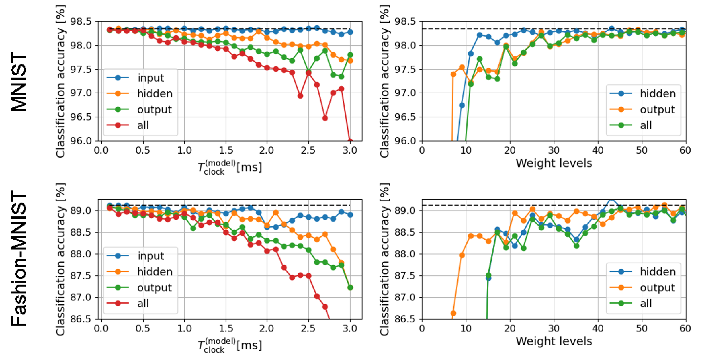
The left panels of Fig. 3 depicts the performance of the SNNs with time-discretized spikes for various values of $T_{\text{clock}}^{\text{(model)}}$. For both the MNIST and Fashion-MNIST datasets, the effects of the time discretization of the spikes at the output layer were more significant than those at the other layers. This can be attributed to the fact that the prediction results obtained by the network are represented by the earliest spike at the output layer. If the real timing difference between the earliest and second earliest spikes is less than $T_{\text{clock}}^{\text{(model)}}$, the network cannot predict the correct label when the timing of the spikes is discretized. The effects of the time discretization of the spike timing were substantially lower for the input layer. This may be because the coding of the input spikes includes “no spike” states, which are inherently robust against timing discretization.

The right panels of Fig. 3 presents the performance of the SNNs when the weights were quantized. In this figure, the horizontal axis represents the number of levels of the quantized weights, given by $\text{max }\left(|w^{(l)}_{ij}|\right)/w^{\text{(min)}}$. We found that performance degradation could be avoided if the number of levels was greater than approximately 20.

Figs. 4 (a) and (b) present the classification accuracy for various values of the lower bound $V_{\text{min}}$ of the membrane potential. Fig. 4 (c) shows the distribution of the minimum value of the membrane potential of the neurons at the output layer, given by

when $V_{\text{min}}$ was not considered. Because the membrane potentials were more likely to take lower values for the MNIST dataset than for the Fashion-MNIST dataset, the SNNs trained on the MNIST dataset were more vulnerable to the value of $V_{\text{min}}$ as indicated in Figs. 4 (a) and (b). We note that the performance was not affected when only the lower bound the membrane potential of neurons in the hidden layer were considered.

One may wonder why the SNNs trained on the MNIST dataset were almost not affected by the lower bound when $V_{\text{min}}$ = -1, even though the average of the minimum voltage $v^{\text{(min)}}$ given by (8) was much lower than -1 as shown in Fig. 4 (c). This is because the minimum values (8) were typically obtained after another neuron was fired, as shown in Fig. 2. To elucidate this fact, Fig. 4 (d) plots the distribution of the minimum membrane potential before the timing of the earliest spike:

We found that a large portion of the minimum membrane potentials given by (9) had distributions that were higher than -0.5.

Fig. 5 depicts the classification accuracy for various values of $\sigma_{V_{\text{th}}}$. We found that the performance of the SNNs was not significantly impaired if $\sigma_{V_{\text{th}}}$ was less than 0.05 for the MNIST and Fashion-MNIST datasets.

We consider an integrate-and-fire model as illustrated in Fig. 6, which is commonly employed in matrix–vector computation [23][22][1][25] and SNNs [19, 17]. The time evolution of the membrane potential represented by the voltage at a capacitor is obtained by Kirchhoff’s current law, as follows:

where $I^{\text{(min)}}$ represents the controllable minimum current, $I_{ij}^{\text{(level)}}$ is an integer, and $C$ is the capacitance. The timing of the firing is obtained as follows:

where $T_{\text{clock}}^{(\text{circuit})}$ is a real number representing the time step of the time-discrete spikes in the circuits.

By setting $I_{ij}^{(l,\text{level})}=w_{ij}^{(l,\text{level})}$, the condition whereby (1) and (10) are equivalent can be obtained as follows:

We used the circuit parameters displayed in Fig. 6 to study the mapping of SNNs to circuits. These values of parameters were determined typically from VLSI design based on the approach of time-domain analog computing with transient states (TACT), in which synapse currents were given by field-effect transistors operating in a subthreshold region [22, 25].

Fig. 7 presents the classification accuracy for various values of $T_{\text{clock}}^{\text{(model)}}$. Note that the value of $w^{\text{(min)}}$ was determined using the values of $T_{\text{clock}}^{\text{(model)}}$ and (13). For the MNIST dataset, the classification accuracy decreased almost monotonically as $T_{\text{clock}}^{\text{(model)}}$ increased. For the Fashion-MNIST dataset, the classification accuracy exhibited a peak around $T_{\text{clock}}^{\text{(model)}}$ = 0.4 ms. The performance of the SNN was mainly affected by the time discretization and weight quantization. To elucidate that, Fig. 7 also depicts the classification accuracy when only the time discretization and the weight quantization were considered and that when only the time discretization or the weight quantization was considered.

As the network could cease its operation after the earliest spike was generated in the output layer, the energy efficiency increased as the average timing of the earliest spike became shorter. Fig. 8 indicates that the average timing of the earliest spike at the output layer decreased as a function of $T_{\text{clock}}^{\text{(model)}}$, because the time steps required to obtain the output spikes was small when $T_{\text{clock}}^{\text{(model)}}$ was large (see Fig. 2) with the same $T_{\text{clock}}^{\text{(circuit)}}$.

The optimal choice of $T_{\text{clock}}^{\text{(model)}}$ was determined by the trade-off between the classification accuracy (Fig. 7) and energy efficiency (Fig. 8). For example, if an accuracy of more than 98% was required with the minimum energy efficiency for the MNIST dataset, the optimal $T_{\text{clock}}^{\text{(model)}}$ would be approximately 0.8 ms.

References

- [1] Bavandpour, M., Mahmoodi, M.R., Strukov, D.B.: Energy-efficient time-domain vector-by-matrix multiplier for neurocomputing and beyond. IEEE Transactions on Circuits and Systems II: Express Briefs (2019)
- [2] Bohte, S.M., Kok, J.N., Poutré, H.L.: Error-backpropagation in temporally encoded networks of spiking neurons. Neurocomputing 48(1), 17–37 (October 2002)
- [3] Comsa, I.M., et al.: Temporal coding in spiking neural networks with alpha synaptic function. In: ICASSP 2020 - 2020 IEEE International Conference on Acoustics, Speech and Signal Processing (ICASSP). pp. 8529–8533 (2020)
- [4] Davies, M., et al.: Loihi: A neuromorphic manycore processor with on-chip learning. IEEE Micro 38(1), 82–99 (2018)
- [5] Diehl, P.U., et al.: Fast-classifying, high-accuracy spiking deep networks through weight and threshold balancing. In: 2015 International Joint Conference on Neural Networks (IJCNN). pp. 1–8 (July 2015)
- [6] Göltz, J., et al.: Fast and deep neuromorphic learning with first-spike coding. In: Proceedings of the Neuro-inspired Computational Elements Workshop. pp. 1–3 (2020)
- [7] Huh, D., Sejnowski, T.J.: Gradient descent for spiking neural networks. In: Advances in Neural Information Processing Systems. vol. 31, pp. 1433–1443 (2018)
- [8] Kheradpisheh, S.R., Masquelier, T.: Temporal backpropagation for spiking neural networks with one spike per neuron. International Journal of Neural Systems 30(6), 2050027 (2020)
- [9] Kheradpisheh, S.R., Mirsadeghi, M., Masquelier, T.: BS4NN: Binarized spiking neural networks with temporal coding and learning. arXiv:2007.04039 (2020)
- [10] Kim, J., Kim, K., Kim, J.J.: Unifying activation-and timing-based learning rules for spiking neural networks. arXiv:2006.02642 (2020)
- [11] Kim, S., Park, S., Na, B., Yoon, S.: Spiking-YOLO: spiking neural network for energy-efficient object detection. In: Proceedings of the AAAI Conference on Artificial Intelligence. vol. 34, pp. 11270–11277 (2020)
- [12] LeCun, Y., Bottou, L., Bengio, Y., Haffner, P.: Gradient-based learning applied to document recognition. Proceedings of the IEEE 86(11), 2278–2324 (November 1998)
- [13] Maass, W.: “Computing with Spiking Neurons,” in Pulsed Neural Networks, chap. 2, pp. 55–85. MIT Press (1999)
- [14] Merolla, P.A., et al.: A million spiking-neuron integrated circuit with a scalable communication network and interface. Science 345(6197), 668–673 (2014)
- [15] Moradi, S., Qiao, N., Stefanini, F., Indiveri, G.: A scalable multicore architecture with heterogeneous memory structures for dynamic neuromorphic asynchronous processors (DYNAPs). IEEE Transactions on Biomedical Circuits and Systems 12(1), 106–122 (Feb 2018)
- [16] Mostafa, H.: Supervised learning based on temporal coding in spiking neural networks. IEEE Transactions on Neural Networks and Learning Systems 29(7), 3227–3235 (July 2018)
- [17] Oh, S., et al.: Hardware implementation of spiking neural networks using time-to-first-spike encoding. arXiv:2006.05033 (2020)
- [18] Pfeiffer, M., Pfeil, T.: Deep learning with spiking neurons: Opportunities and challenges. Frontiers in Neuroscience 12(774), 1–18 (2018)
- [19] Sakemi, Y., Morino, K., Morie, T., Aihara, K.: A supervised learning algorithm for multilayer spiking neural networks based on temporal coding toward energy-efficient VLSI processor design. arXiv:2001.05348 (2020)
- [20] Sze, V., Chen, Y., Yang, T., Emer, J.S.: Efficient processing of deep neural networks: A tutorial and survey. Proceedings of the IEEE 105(12), 2295–2329 (2017)
- [21] Tavanaei, A., Ghodrati, M., Kheradpisheh, S.R., Masquelier, T., Maida, A.: Deep learning in spiking neural networks. Neural Networks 111, 47–63 (2019)
- [22] Wang, Q., Tamukoh, H., Morie, T.: A time-domain analog weighted-sum calculation model for extremely low power VLSI implementation of multi-layer neural networks. arXiv:1810.06819 (2018)
- [23] Wang, Q., Tamukoh, H., Morie, T.: Time-domain weighted-sum calculation for ultimately low power VLSI neural networks. In: Neural Information Processing. vol. 9947, pp. 240–247 (September 2016)
- [24] Xiao, H., Rasul, K., Vollgraf, R.: Fashion-MNIST: a novel image dataset for benchmarking machine learning algorithms. arXiv:1708.07747 (2017)
- [25] Yamaguchi, M., Iwamoto, G., Nishimura, Y., Tamukoh, H., Morie, T.: An energy-efficient time-domain analog cmos binaryconnect neural network processor based on a pulse-width modulation approach. IEEE Access 9, 2644–2654 (2020)