Prediction-Free, Real-Time Flexible Control of Tidal Lagoons through Proximal Policy Optimisation: A Case Study for the Swansea LagoonJournal: Ocean Engineering
Abstract
Tidal Range Structures (TRS) have been considered for large-scale electricity generation for their potential ability to produce reasonably predictable energy without the emission of greenhouse gases. Once the main forcing components for driving the tides have deterministic dynamics, the available energy in a given TRS has been estimated, through analytical and numerical optimisation routines, as a mostly predictable event. This constraint imposes state-of-art flexible operation methods to rely on tidal predictions to infer best operational strategies for TRS, with the additional cost of requiring to run optimisation routines for every new tide. In this paper, a Deep Reinforcement Learning approach (Proximal Policy Optimisation through Unity ML-Agents) is introduced to perform automatic operation of TRS. For validation, the performance of the proposed method is compared with six different operation optimisation approaches devised from the literature, utilising the Swansea Bay Tidal Lagoon as a case study. We show that our approach is successful in maximising energy generation through an optimised operational policy of turbines and sluices, yielding competitive results with state-of-art optimisation strategies, with the clear advantages of requiring training once and performing real-time automatic control of TRS with measured ocean data only.
Keywords:
marine renewable energy , tidal energy , tidal power plants , machine learning , deep reinforcement learning , proximal policy optimisation1 Introduction
In recent years, concerns about climate change combined with political and social pressures have pushed the world to increase the installed capacity of renewable energy sources (wind, solar, bioenergy and hydro), allowing renewable energy to account for 28% of global energy generation in 2020 [1]. While significant progress has been made in expanding solar and wind resources, tidal energy remains practically untapped. As of today, only two successful large Tidal Range Structure (TRS) projects have been built, namely, La Rance (France) and Lake Sihwa (South Korea), with 240 and 254 of installed capacity, respectively [2].
A review by UK’s ex-minister of energy [3] has drawn attention to TRS as a competitive choice among renewables. In his report, the construction of “small-scale” TRS, such as the Swansea Bay Tidal Lagoon (our case study), is suggested as a pathfinder project before moving to larger-scale TRS [4, 5, 6]. The report also emphasises that TRS have proposed lifetimes of operation of 120 years – far surpassing any other renewable energy type, allowing for very low electricity cost for years. As an example, La Rance, which is in operation for 55 years, took 20 years to amortise the initial investment, generating energy at competitive cost of nuclear or offshore wind sources [7, 3].
Among the challenges faced in TRS deployment is the optimisation of energy generation through the operation of hydraulic structures (turbines and sluices), which increases the utilisation factor (ratio of actual energy generated to installed capacity). Although the current literature has advanced in increasing theoretical power generation capabilities of TRS [2, 8, 9], there is room for improvement, considering that state-of-art (flexible operation) optimisation methods (i) can be computationally time expensive and (ii) do not perform real-time control, relying on accurate tidal prediction techniques. In view of this, we propose the usage of Deep Reinforcement Learning (DRL) methods, more specifically Proximal Policy Optimisation (PPO) through the Unity ML-Agents package [10], which enables state-of-art energy generation of TRS (on par with best optimisation routines) through the real-time control of turbines and sluices. DRL was chosen among machine learning techniques due to the nature of our problem, which involves sequential decision-making of a reactive environment (lagoon water levels vary depending on the operation of hydraulic structures) with the goal of maximising expected return (energy), and also because a target optimal operation of the tidal lagoon is not known “a priori” – a requirement for supervised learning techniques. After training, our method shows consistent performance, regardless of test data used, not requiring future tidal predictions or re-training the DRL agent. To date, this is the first flexible operation optimisation approach in the literature that can maximise TRS energy generation without such constraints. A 0D model of the Swansea Bay Tidal Lagoon is utilised to compare our DRL method with six optimisation baselines devised from the literature [11, 12].
After related work (Section 2), this paper is divided in four parts. In the first part, we explain how tidal barrages extract energy from the tides through the lenses of classical and variant operation approaches. In the second part, we cover the theory behind DRL, more specifically on the PPO algorithm that is used in this study. In the third part, we cover our agent-environment setup, modelled with the Unity ML-Agents package (Table S1, Supplementary Material). In the final part, an experimental study contrasting our results with six baselines is presented and discussed.
2 Related Work
State-of-art optimisation methods for TRS estimate the available energy in such systems by operating the tidal lagoon hydraulic structures through flexible operational strategies (adaptive, according to tidal amplitudes and lagoon water levels for sequential tidal cycles [12, 11]). With the assumption of well predictable tides, flexible operation of turbines and sluices can be inferred by “looking–ahead” through harmonic or numerical tidal prediction methods [13] and applying the acquired operation to the real, measured ocean – a procedure that needs to be repeated for every new tide. In fact, and to the best of our knowledge, the requirement of accurate future tidal predictions (concurrent with measured data and up to a multiple of half-tidal cycles into the future) has been the basis for all optimisation routines developed for enabling flexible operation [14, 12, 11, 15, 16, 2, 17]. This constraint can be a problem when future tidal predictions are unavailable, unreliable, have some associated validation cost [18] or are regulated by private companies or government agencies.
State-of-art optimisation routines in the literature utilise either grid search (a brute-force approach), gradient-based, global optimisation [12, 11, 16] and, more recently, genetic algorithm methods [17] to optimise the operation of TRS. As a basis of comparison with our DRL agent, two non-flexible and four flexible state-of-art baselines devised from [11, 12] are modelled utilising grid search and global optimisation methods.
3 Tidal Power Overview
TRS extract power by artificially inducing a water head difference between the ocean and an impounded area. By allowing water to flow through the hydraulic structures into an artificial impoundment, the incoming tide (flood tide) is confined within the lagoon at high level (holding stage). Then, during the receding tide (ebb tide), power generation begins when a high operational head () is established between the basin and ocean [19]. Power generation then stops when a minimum operational head () is achieved. A sluicing sequence immediately follows, where idling turbines and sluices allow water to flow in order to increase lagoon tidal range for the next operation. Following the same procedure, generating energy is also possible during the flood tide, although with reduced efficiency due to turbines usually being ebb-oriented [11]. From the literature, operational strategies that allow for power generation to occur during flood and ebb tides are called “two-way scheme” operation [19]. Operational modes for controlling TRS in a “two-way scheme” are shown in Fig. 1 and detailed in Table 1.

| Operational Mode | Description |
|---|---|
| Ebb Gen: | Power generation during receding tide |
| Flood Gen: | Power generation during incoming tide |
| Sluicing: | Operate sluice gates and/or idle turbines |
| Holding: | Stop operation of all hydraulic structures |
| Operational Mode | Turbines | Sluices | Power Gen. |
|---|---|---|---|
| Ebb Gen: | On | Off | Yes (if ) |
| Flood Gen: | On | Off | Yes (if ) |
| Sluicing: | On | On | No |
| Holding: | Off | Off | No |
TRS turbines can be operated to either generate energy or to increase flow rates through the barrage during sluicing stage (idle operation of turbines). Also, a minimum head , usually in the range [20], is required for the turbine to generate energy ( in this study). Considering that the holding stage begins automatically when the difference between ocean and lagoon is negligible, and that power generation is not possible with head differences below , the classic operation of tidal lagoons [19] is reduced to two variables: and . As seen in Fig. 1, pairs and occur every half-tide period, when ocean oscillates between its valleys and peaks.
A slight modification of the discussed classical operation allows for opening the sluice gates at the end of “flood” and “ebb” generation stages [21, 11] independently of , with the possibility of increasing power generation (increased lagoon tidal range when starting the next “ebb” or “flood” stages). This variant operation requires 3 control variables every half-tide: , and (sluice gate starting head). The water level variations within the lagoon, following classic and variant operations of hydraulic structures, can be seen in Fig. 1. Tables 2 and 3 show all possible combined operations of turbines and sluices, with resulting power generation, for each control stage in classic and variant operations, respectively. Classic and variant approaches to operate TRS are used in the optimisation routines of our baselines in Section 6.1.
| Operational Mode | Turbines | Sluices | Power Gen. |
|---|---|---|---|
| Ebb Gen: | On | Off/On | Yes (if ) |
| Flood Gen: | On | Off/On | Yes (if ) |
| Sluicing: | On | Off/On | No |
| Holding: | Off | Off | No |
3.1 Tidal Lagoon Simulation - 0D Model
In order to estimate the available energy of two-way operational strategies, analytical or numerical models (0D to 3D) can be considered. When the goal is the optimisation of TRS operation for maximising energy generation, 0D models are usually chosen, given their computational efficiency, and the fact that for “small-scale” projects, such as the Swansea Bay Tidal Lagoon, 0D models present good agreement with more complex finite-element 2D models [22, 11, 12, 2, 23]. 0D models are derived from conservation of mass:
| (1) |
where is the water level (in meters) inside the lagoon, is the total directional water flow rate () from both sluices and turbines and is the variable lagoon area (). From Eq. 1, the lagoon water level at the following time-step () can be calculated by a backward finite difference method:
| (2) |
where is the water level at time-step and the discretized time ( in this work).
3.2 Turbine and Sluice Parametrization
From 0D to 2D models, studies show that flow rate and power from turbines can be approximated with the parametrization of experimental results [24, 20, 25]. For this work, the equations describing flow and power for low head bulb turbines were based on experimental results from Andritz Hydro [25]. The edited Andritz chart shown in Fig. 2 demonstrates how turbine unit speed and specific unit discharge (obtained experimentally) are related. The graph also shows wicket gate and running blade openings ( and , in degrees), and iso-efficiency curves .

By specifying the parameters of the turbine: diameter , number of generating poles and grid frequency , the turbine rotation () is obtained from . Furthermore, unit speed , turbine flow rate and power output are calculated as:
| (3) |
| (4) |
| (5) |
is the head difference between ocean and lagoon, the seawater density (), the gravity acceleration () and is the product of other efficiencies shown in Table 4.
| TRS Efficiencies | (%) |
|---|---|
| Generator | 97 |
| Transformer | 99.5 |
| Water friction | 95 |
| Gear box/drive train | 97.2 |
| Turbine availability | 95 |
| Turbine orientation (Flood Gen. only) [11] | 90 |
When is available, is estimated directly from Eq. (3). For calculating and , and are obtained experimentally by adjusting the opening of the wicket gates (), the pitch angle of the runner blades () and crossing the values with the obtained (see Fig. 2). In order to choose appropriate values for and , a parameterized curve of maximum power output was drawn over Fig. 2 (blue line) by following the path where the product between , and is maximised. If we assume and are automatically adjusted to always be in the maximum power output curve, then and become functions of , as shown in Eq. (6) and (7):
| (6) | ||||
and
| (7) |
For simulating sluice gates, the barrage model utilises the orifice equation, so that the flow rate is a function of [19, 21]:
| (8) |
where is the discharge coefficient for sluices (equal to one in this study, following [11]), and the sluice area.
When generating energy, turbines use Eq. (4) for estimating flow rate through the barrage. On the other hand, when operating in “idling” mode, turbines use equation Eq. (8), with [11].
When starting or stopping either turbines or sluices, the literature has used sinusoidal ramp functions for simulating the smooth transition of flow output as [11, 22], where , (around 15 to 20 [11, 26]), and is the time when the current operation was triggered. Since this is a heuristic method, a simpler transition function (named “momentum ramp”) is proposed in this work:
| (9) |
is the estimated flow rate at the next time-step, is the total flow rate calculated from turbines and sluice equations (Eq. (4, 8)), a dimensionless hyperparameter that controls the intensity of flow rate update per time-step, is the flow rate at time-step “” and .
The “momentum ramp” is applied every time-step during simulation. This not only simplifies the code, but facilitates training, since sluice opening is treated as a continuous control problem (Section 5.2). In this work we set , which guarantees a precision of for a 15 time interval with .
4 Reinforcement Learning Overview
As shown in the work of Sutton and Barto [27], a reinforcement learning (RL) problem can be mathematically formalised as a Markov Decision Process (MDP). In an MDP, an agent interacts with an environment through actions (), and these actions lead to new environmental states () and possible rewards () for the agent. The quantities , and are random variables, with well-defined probability distributions. A general agent-environment MDP framework can be visualised in Fig. 3.

By sampling multiple time-steps , observations () of the agent-environment interaction are organised as a sequence of state-action, next reward triples:
| (10) |
where, are instances of the random variables (, and ). The sequence of state-action pairs defines a trajectory :
| (11) |
Also, in an MDP, we can say that the probabilities of and are completely conditioned on the preceding state and action ( and ), that is:
| (12) |
The probability distribution of Eq. (12) defines the dynamics of the MDP. It can also be manipulated to yield the state-action-transition probability distribution (which is just the sum of probabilities over all possible future rewards):
| (13) |
For estimating Eq. (13) for a given state, we also need to condition an action. In non-deterministic scenarios, the selection of possible actions by the agent is a stochastic process, defined by a conditional probability distribution (known as policy) of the form:
| (14) |
Using Eq. (13,14), the probability distribution of starting in a state and ending in , given a policy, can be estimated as:
| (15) |
With a defined policy, we can sum the observed rewards for each state-action pair (as shown in Eq. (10)) and calculate a total return at time-step :
| (16) |
where is a discount factor between 0 and 1.
The objective of reinforcement learning problems is to find an optimal policy , that maximises the expected return of rewards conditioned on any initial state, i.e.
| (17) |
4.1 Proximal Policy Optimisation (PPO)
Once the reinforcement learning problem is formalised as an MDP, several algorithms can be used for finding an optimal control policy . In this work, the process of finding has been achieved through Proximal Policy Optimisation (PPO) [28], built in the Unity ML-Agents package. PPO was shown to outperform several other “on-policy” gradient methods [28] and is one of the preferred methods for control optimisation when the cost of acquiring new data is low [29]. Furthermore, a revised and up-to date PPO algorithm is already implemented in Unity ML-Agents. Nevertheless, for sake of completeness, we present in this section the mathematical derivation of the PPO method. The designing of the TRS operation as an MDP is shown in Section 5.2.
Differently from approaches that try to infer the policy through state-value or action-value functions (e.g. Deep Q-Network) [30], PPO uses an “on-policy” approach that maximises the expected sum of rewards by improving its current policy – smoothly shifting the probability density function estimate of the policy towards . The PPO algorithm is an updated form of Policy Gradients. As TRPO (Trust Region Policy optimisation) [31], it tries to increase sample efficiency (re-using data from previous policies), while constraining gradient steps to a trust region. It is also actor-critic, since it utilises an estimate of the state-value function for its baseline [32]. An overview of Policy Gradients and PPO is presented below.
4.1.1 Policy Gradients
Policy gradient methods rely on the fact that a stochastic policy can be parameterized by an “actor” neural network with weights (simplified as going forward). As represented in Fig. 4, this neural network receives a vector state representation of . For the case of discrete actions, the neural network outputs the probabilities of each possible action in that state using a softmax layer. For continuous actions, each node in the last layer outputs the moments of a multivariate Gaussian distribution of the form [33, 34]:
| (18) |
where and are the parameterized mean and co-variance matrices, respectively. While training, actions are randomly sampled from the distribution to favour exploration. During testing, is taken as the optimum action for each input state .

Considering a trajectory , the expected return of following a parameterized policy is , where
| (19) |
and is the reward from taking action from state . We also note that represents the undiscounted return following a sampled trajectory for a time horizon . With these considerations, finding an optimal policy can be viewed as tuning to maximise , i.e. to perform gradient ascent of :
| (20) |
A sample based estimate for assumes the form:
| (21) |
where is the number of sampled trajectories from the “actor” neural network. For vanilla policy gradient methods [35], following a trajectory , we get
| (22) |
| (23) |
, parameterized by a “critic” neural network, is the estimate for the value function of being in state and following policy thereafter; is the discounted future return of following the chosen trajectory, from time ; and is the advantage estimate of taking this trajectory in respect to the current estimate of . A complete derivation of can be seen in [35].
4.1.2 Clipped Surrogate Loss derivation for PPO
In order to increase sampling efficiency [36], importance sampling can be used to rewrite the gradient term in Eq.( 21) as:
| (24) |
Eq.( 24) importance sampling form allows for re-utilising samples from an older policy to perform gradient ascent steps, when refining a new policy. It is obtained when differentiating the Surrogate Loss:
| (25) |
where is a probability ratio.
While in TRPO [31] the maximization of the surrogate loss from Eq.( 25) is subjected to a Kullback–Leibler divergence constraint, in PPO [28] the surrogate loss is constrained through a clipping procedure, yielding the clipped surrogate loss objective:
| (26) |
where is a hyperparameter that limits large policy updates.
To further reduce variance when estimating the advantage, [28, 32] utilise a truncated version of generalized advantage estimation [37], where is estimated as
| (27) |
where is a time index within the sampled trajectory time horizon , is a hyperparameter that performs the exponential weighted average of k-step estimators of the returns [37], and .
When utilising shared parameters for the “actor” and “critic” neural networks (as is the case with this work), the loss function needs to be augmented with a value function error term [28]. To ensure exploration, an entropy term “” is also added. Finally, the loss function to be maximised at each iteration becomes:
| (28) |
For this study, Unity ML-Agents package fixes [38], is a hyperparameter controlling the entropy bonus magnitude , and is a clipped, squared-error loss between the estimate of the state-value function and the actual return value obtained when following a trajectory [28]. The implementation of in Unity ML-Agents is seen in [38].
Additionally, parallel training can also be implemented as a way of substituting experience replay by running the policy on multiple instances of the environment. By guaranteeing that each environment starts in a random initial state during training, this parallelism helps decorrelate the sampled data, stabilising learning [39].
5 Agent-Environment Setup
5.1 Unity ML-Agents
The Unity3D graphics engine is a popular game developing environment that has been used to create games and simulations in 2D and 3D since its debut in 2005. It has received widespread adoption in other areas as well, such as architecture, engineering and construction [10].
5.2 Agent-Environment MDP Modelling and Training
To formalise TRS operation as a RL problem (and subsequently solve the RL problem through PPO) we need to design an MDP in Unity ML-Agents with environment, agent, actions, states and reward components.
By creating simple representative 3D models for turbines, sluices, ocean and lagoon, a training environment simulating TRS for our MDP is created in Unity3D and then imported to a Unity ML-Agents project. In this environment, the equations for simulating flow operation through the lagoon, when operating sluices and turbines, are extracted from the 0D model representation, detailed in Section 3.2. In order to choose appropriate parameters for operating our environment, we follow literature representations suggested by [11, 22, 12], for the Swansea Bay Tidal Lagoon project. The chosen parameters are shown in Table 5. A variable lagoon surface area, digitized from [12], is also utilised. For ease of visualisation, the 3D representations of sluice and turbine change colours depending on the operational mode chosen by the agent. For the turbine, green represents power generation mode, orange – idling mode and black – offline mode (zero flow rate). Similarly, sluices change colour between orange and black for sluicing and offline modes, respectively. Fig. 5 shows a capture of the Unity ML-Agents MDP environment representation for the Swansea Bay tidal Lagoon during ebb generation, with the representative models for sluice and turbines in offline and power generation modes, respectively. Ocean and Lagoon surface level motion are also represented.
| of Turbines | |
| of | |
| Grid frequency | |
| Turbine Diameter () | |
| Sluice Area () |

Additionally, in this proposed MDP, the actor-critic agent is defined as an operator responsible for controlling turbine and sluice operational modes through actions (policy network node outputs ), according to a vector of input states . outputs can be discrete or continuous. In this work, continuous outputs are chosen, reducing the number of nodes in the last layer, and consequently, the complexity of the neural network. There are node outputs that determine turbine and sluice operation every 15 of the environment simulation. The 15 window (MDP time-step) was selected for this work since the time usually associated with the opening/closing of hydraulic structures lies in the range [11, 26].
Each node in the last layer outputs a value between and , and the resulting actions are computed in a hierarchical fashion. The first node determines the number of turbines set to power generation mode ( or ), depending if the node output is below or above a threshold (), i.e. if the node outputs a value below the threshold, no turbines will be generating energy, otherwise, all turbines are set to power generating mode. Therefore, if no turbines are set to power generation, are available for other operational modes (idling or offline).
The second node selects the number of idling turbines just as the first node, if the number of turbines available is . Otherwise the number of idling turbines is , independent of this node output. If no turbine is selected for power generation or idling modes, all turbines are set offline. Therefore, the first two nodes control turbines through discrete actions.
The third and final node outputs the opening area of the sluice gates. Since any value between can be chosen by the neural network, the momentum ramp function (Section 3.2) is applied to the outputted flow rate every time-step, ensuring smooth flow rate transitions, independently of the opening sluice area set by the agent.
Beyond reducing the number of node outputs, this configuration also allows for having the sluice operation independent of turbine operation. All possible operational modes for turbines and sluices as a function of node output () are shown in Tables 6 and 7, respectively.
| Node 1 | Node 2 | Discrete Turbine Control |
|---|---|---|
| Offline Mode | ||
| Idling Mode | ||
| Power Generation Mode | ||
| Power Generation Mode |
| Node 3 | Continuous Sluice Control |
|---|---|
| Sluicing Mode (Available sluice area = ) | |
| Offline Mode (Available sluice area = 0) |
The actions selected by the agent are a function of the input states . In this work, these states are the water levels of ocean and lagoon, plus current operational mode of turbines and sluices, for current and previous MDP time-steps (Table 8). Finally, the reward received by the agent equals the accumulated energy generated by the turbines, for every 15 .
| States (at times and ) | Units |
|---|---|
| Ocean water level | meters (float) |
| Lagoon water level | meters (float) |
| Number of online turbines | 0, or 16 (integer) |
| Number of idling turbines | 0, or 16 (integer) |
| Sluice gate opening area | 0 to 1 (float) |
For stabilising and speeding up training, parallel training is performed with 64 copies of the environment (Fig. 6), while episodes are set to month of duration. During training, each environment instance requires a representative ocean input at the location where the Swansea Lagoon is planned to be constructed ( ). Ideally, ocean measurements could be used as training data. However, due to the lack of sufficient measured data (Section 6.1), it is not possible to train the agent until reasonable performance is reached. Instead, an artificial tide signal to simulate the ocean is created by summing the major sinusoidal tide constituents (due to gravitational pull of the Moon and Sun). Although we are not accounting for other less predictable local wave motions (e.g. wind waves), the artificial ocean input representation is sufficient for enabling the agent to converge to an optimal policy. A major advantage of this approach is the fact that we can generate any amount of input data required for training the agent.

The tide constituent’s amplitudes of the simulated ocean utilised in this work (Table 9), were obtained from a numerical simulation, at the location of Swansea Bay Tidal Lagoon, by [11]. The periods for each constituent were obtained by [40]. The final equation for simulating the ocean can be seen in Eq. (29).
| (29) | ||||
where , , and are angular frequencies (rad/s) of each tidal component, and , , and are random phase lags in the range , generated for each environment instance during parallel training when starting an episode, which allow for learning more generalised scenarios.
| Ocean tide constituent | Amplitude (m) | Period (hr) |
|---|---|---|
The designed MDP is solved through the PPO algorithm (Section 4.1). A flow-chart, illustrating the agent’s training stage through the PPO algorithm in Unity ML-Agents, is presented in Fig. 7. Training occurs until a “max-steps” number of observations are sampled. For reproducibility, Table S2 in the Supplementary Material showcases the PPO hyperparameters utilised during training.

After training, the policy (actor) neural network receives input states and outputs optimum values, following a policy that maximises energy generation. During testing, this means that the agent receives real ocean measurements as input, performing real-time flexible control of turbines and sluices.
6 Experiments
In this section we compare our DRL trained agent performance against state-of-the-art optimisation routines. Codes for reproducibility can be made available under request to the corresponding author.
6.1 Test Data and Baselines optimisation
For comparing our DRL agent performance against conventional optimisation routines, we model six baselines devised from the recent literature [11, 12] and compare the energy generated in a month for each method. All baselines in this work consider the operation of the Swansea Bay tidal lagoon either through classic or variant “two-way scheme” methods, as detailed in Section 3.
Regarding test data for baselines and trained agent, we utilise all tide gauge ocean measurements available from the British Oceanographic Data Centre (BODC) at Mumbles Station [41], located at the edge of Swansea Bay. The obtained measurements of ocean elevation are recorded every 15 in a table, for the years of and the range . Before utilising the data, a preprocessing step is performed so that data flagged as “improbable”, “null value” and “interpolated” by BODC are not considered. After this step we retain months of usable, non-overlapping, test data. The preprocessing step ensures a conservative comparison between baselines and our trained agent, since it considers scenarios where tidal predictions had a good match with measured data.
Tidal predictions for the same 26 months are also provided by BODC in the same data-set. For each month, baseline optimisation routines utilise tidal predictions for capturing operational head values , and (when considered) that optimise power generation. These operational head values are then applied to the measured ocean test data, so that comparisons between baselines and trained agent can be made. Baselines, in increasing order of optimisation complexity, are described next:
- 1.
CH (Constant Heads): Best, constant and are picked for extracting energy during a whole month [14].
- 2.
CHV (Constant Heads, with variant operation): Best, constant heads , and are picked for extracting energy during a whole month.
- 3.
EHT (Every Half-Tide): optimised pairs of and are picked for every consecutive half-tide. Proposed by [12].
- 4.
EHTV (Every Half-Tide, with variant operation): optimised , and are picked for every consecutive half-tide.
- 5.
EHN (Every Half-Tide and Next): optimised and are picked for every half-tide, considering the best and for the next half-tide as well. Proposed by [12].
- 6.
EHNV (Every Half-Tide and Next, with variant operation): optimised , and are picked for every half-tide, considering the best , and for the next half-tide as well.
All variant optimisation methods are augmented through the addition of independent sluice head operation . This modification we are introducing is inspired by the work of [21, 11]. CH and CHV perform non-flexible operation, while EHT, EHTV, EHN and EHNV perform state-of-art flexible operation. A summary detailing each baseline operational heads and method is shown in Table 10.
| Constant Head | Every Half-Tide | Every Half-Tide and Next | ||||
|---|---|---|---|---|---|---|
| CH | CHV | EHT | EHTV | EHN | EHNV | |
| ✓ | ✓ | ✓ | ✓ | ✓ | ✓ | |
| ✓ | ✓ | ✓ | ✓ | ✓ | ✓ | |
| ✓ | ✓ | ✓ | ||||
| non-flexible operation | ✓ | ✓ | ||||
| flexible operation | ✓ | ✓ | ✓ | ✓ | ||
All baselines, except EHNV, are optimised with a grid search optimisation algorithm, which iteratively increases its search resolution until convergence. Initial search resolution starts with meter, with optimisation heads , and (when considered) within ranges , and , respectively. After the first run, search resolution is halved and the algorithm performs a brute-force search around the best previous configuration attained. The latter procedure is repeated until final search resolution is lower than .
EHNV requires a different optimisation approach due to its high computational time when utilising the previous grid search method. For this case we utilise the stochastic global optimisation algorithm basin-hopping [42] from Scipy package [43], with COBYLA as a local minimizer [44]. Basin-hopping was chosen for its efficiency when solving smooth function problems with several local minima separated by large barriers [45]. The local minimizer COBYLA is a nonlinear derivative–free constrained optimisation that uses a linear approximation approach. Even though basin-hopping is not guaranteed to converge to a global optimum, EHNV is shown to be, on average, the best baseline method for energy generation.
6.2 Agent Performance Evaluation
Following hyperparameter tuning, we trained the agent for steps, until convergence. The cumulative reward (energy) per month (episode) during parallel training, averaged for the 64 instances of the lagoon environment, is shown in Fig. 8. The log-representation insert highlights the two-step plateau that is observed when converging to an optimal strategy. After starting in a total random strategy, the cumulative reward received by the agent increases until reaching an intermediate plateau at around steps, where the agent learns the strategy of operating mostly the turbines, while keeping sluices practically offline during ebb generation. Then, after about steps, the cumulative reward starts increasing again. The second plateau stabilises around steps, with a cumulative reward approximately 25% higher than the first plateau – a gain allowed by (i) a flexible operational strategy learnt by the agent, that adjust TRS operation according to tidal range (ii) the smart usage of the sluicing mode, as discussed below in test results. Videos showcasing the strategic operation developed for both plateaus are available in the Supplementary Material.

For test data, we utilise months of real ocean measurements from BODC. These months are presented and numbered in Table S3, while Table S4 (Supplementary Material) compares the amount of energy obtained in the numbered months between our trained agent (performing real-time flexible control) and the baselines. A block diagram representing the trained agent test stage for this work, while using ocean water level (WL) measurements, is shown in Fig. 9. The averaged monthly energy attained for all methods is shown in Fig. 10.


For the baselines, CH and CHV present the worst performance, since constant operational heads cannot account for the varying ocean amplitudes in a month (about to in our test set). Furthermore, baselines with variant operation outputted more energy in average than their classical counterparts. Finally, “half-tide and next” approaches showed very small improvements () when compared to “half-tide” methods, while requiring much greater () computational time (Tables S5 and S6, Supplementary Material).
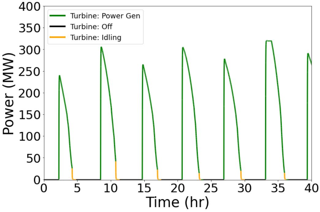
For the trained agent, Fig. 11 show operational test results of power generation and lagoon water levels for one month of measured ocean data (starting with initial lagoon water level at mean sea level). We note that the agent quickly converges to an optimal energy generation strategy for sequential tidal cycles, independent of tidal range input – a characteristic of state-of-art flexible operation [12]. Furthermore, Figs. 12 and 13 showcase detailed results of real-time control on test data. Apart from ocean water levels, results are coloured according to actions taken by the agent for turbines and sluices, respectively, as defined in Section 5.2. More specifically, Figs. 12(a) and 13(a) show lagoon water level variations, while Fig. 12(c), 12(b) and 13(b) show power generation, turbine and sluice flow rates. From the sequence of actions taken, we see that the agent arrives at a policy with independent operation of sluices, i.e. the variant operation of TRS, which was shown to be a better strategy than the classical operation in our baseline comparison. A summary of our method accomplishments in comparison with state-of-art baselines is shown in Table 11.




| CH | CHVa | EHT | EHTVa | EHN | EHNVa | DRL Agent | |
| [14] | [12] | [12] | (our work) | ||||
| real-time flexible control | ✓ | ||||||
| prediction-free approach | ✓ | ||||||
| variant lagoon operation | ✓ | ✓ | ✓ | ✓ | |||
| state-of-art performanceb | ✓ | ✓ | ✓ | ✓ | ✓ | ||
| a optimisation routines with variant operation of tidal lagoons. Augmentation inspired by [11, 21] | |||||||
| b Equivalent outputs, in average, within the error bars (Fig. 10). | |||||||
Our agent managed very competitive energy outputs, staying on average within of the best baseline (EHNV). Indeed, for all months tested, our agent performed optimally, outputting better results than the state-of-art EHN method for 22 out of 26 months (Table S4, Supplementary Material), within a margin in worst scenarios. We note that this novel result was obtained by training the agent once with a simple artificial ocean input, in contrast with the baselines that require future tidal predictions and being re-run for every new tide.
7 Conclusions
In this work, we have shown that Proximal Policy Optimisation (a DRL method) can be used for real-time flexible control of Tidal Range Structures after training with artificially generated tide signals. Our DRL agent implementation was then compared against state-of-art optimisation approaches devised from the literature, yielding competitive results for all test data utilised. Our results were obtained in a conservative setting, i.e., when available tidal measurements had good agreement with tidal predictions (a requirement for state-of-art approaches).
We have chosen the Swansea Bay Tidal Lagoon for our analysis, given its status as a pathfinder project for larger tidal lagoon projects. We show that our novel approach obtains optimal energy generation from measured tidal data only, through an optimised control policy of turbines and sluices, which are operated independently by the trained DRL agent. Our method shows promising advancements over state-of-art optimisation approaches since it (i) performs real-time flexible control with equivalent energy generation, (ii) does not require future tidal predictions, and (iii) needs to be trained a single time only.
Owing to its characteristic features, the method introduced here shall be of wide applicability to achieve optimal energy generation of TRS in cases where future tidal predictions are unreliable or not available. Possible extensions of this work include more sophisticated cases, such as through the introduction of pumping capabilities and/or demand-oriented operation (where the goal is maximising revenue). For such cases, the increase in both the degrees of freedom for the agent’s actions and stochasticity from the input signal could further emphasise the advantage of a DRL real-time operation of TRS over current state-of-art methods.
Acknowledgments
We would like to thank the Brazilian agencies Coordenação de Aperfeiçoamento de Pessoal de Ensino Superior (CAPES) and Conselho Nacional de Desenvolvimento Científico e Tecnológico (CNPq) for providing funding for this research.
References
- [1]
P. IEA, Global
Energy Review 2020 (April 2020, accessed January 10, 2021).
URL https://www.iea.org/reports/global-energy-review-2020 - [2] S. P. Neill, A. Angeloudis, P. E. Robins, I. Walkington, S. L. Ward, I. Masters, M. J. Lewis, M. Piano, A. Avdis, M. D. Piggott, et al., Tidal range energy resource and optimization–past perspectives and future challenges, Renewable Energy 127 (2018) 763–778.
- [3] C. Hendry, The role of tidal lagoons, Final Report (2016) 67–75.
- [4] S. Waters, G. Aggidis, A world first: Swansea bay tidal lagoon in review, Renewable and Sustainable Energy Reviews 56 (2016) 916–921.
- [5] S. Petley, G. Aggidis, Swansea bay tidal lagoon annual energy estimation, Ocean Engineering 111 (2016) 348–357.
- [6] R. Burrows, I. Walkington, N. Yates, T. Hedges, J. Wolf, J. Holt, The tidal range energy potential of the west coast of the united kingdom, Applied Ocean Research 31 (4) (2009) 229–238.
- [7]
S. Evans,
La
Rance: learning from the world’s oldest tidal project (October 4th, 2019,
accessed January 10, 2021).
URL https://www.power-technology.com/features/la-rance-learning-from-the-worlds-oldest-tidal-project/ - [8] S. Waters, G. Aggidis, Tidal range technologies and state of the art in review, Renewable and Sustainable Energy Reviews 59 (2016) 514–529.
- [9] A. Ghaedi, H. Gorginpour, Generated power enhancement of the barrage type tidal power plants, Ocean Engineering 226 (2021) 108787.
- [10] A. Juliani, V.-P. Berges, E. Vckay, Y. Gao, H. Henry, M. Mattar, D. Lange, Unity: A general platform for intelligent agents, arXiv preprint arXiv:1809.02627 (2018).
- [11] A. Angeloudis, S. C. Kramer, A. Avdis, M. D. Piggott, Optimising tidal range power plant operation, Applied energy 212 (2018) 680–690.
- [12] J. Xue, R. Ahmadian, R. A. Falconer, Optimising the operation of tidal range schemes, Energies 12 (15) (2019) 2870.
- [13] G. D. Egbert, R. D. Ray, Tidal prediction, Journal of Marine Research 75 (3) (2017) 189–237.
- [14] R. Ahmadian, J. Xue, R. A. Falconer, N. Hanousek, Optimisation of tidal range schemes, in: Proceedings of the 12th European Wave and Tidal Energy Conference, 2017, p. 1059.
- [15] J. Xue, R. Ahmadian, O. Jones, Genetic algorithm in tidal range schemes’ optimisation, Energy (2020) 117496.
- [16] F. Harcourt, A. Angeloudis, M. D. Piggott, Utilising the flexible generation potential of tidal range power plants to optimise economic value, Applied Energy 237 (2019) 873–884.
- [17] J. Xue, R. Ahmadian, O. Jones, R. A. Falconer, Design of tidal range energy generation schemes using a genetic algorithm model, Applied Energy 286 (2021) 116506.
- [18] E. Medina-Lopez, D. McMillan, J. Lazic, E. Hart, S. Zen, A. Angeloudis, E. Bannon, J. Browell, S. Dorling, R. Dorrell, et al., Satellite data for the offshore renewable energy sector: synergies and innovation opportunities, arXiv preprint arXiv:2103.00872 (2021).
- [19] D. Prandle., Simple theory for designing tidal power schemes, Advances in Water Resources 7 (1) (1984) 21–27.
- [20] G. A. Aggidis, D. S. Benzon, Operational optimisation of a tidal barrage across the mersey estuary using 0-d modelling, Ocean Engineering 66 (2013) 69–81.
- [21] C. Baker, Tidal Power, Institution of Engineering and Technology (1711), (1991).
- [22] A. Angeloudis, M. Piggott, S. C. Kramer, A. Avdis, D. Coles, M. Christou, Comparison of 0-d, 1-d and 2-d model capabilities for tidal range energy resource assessments, EarthArXiv (2017).
- [23] A. M. Schnabl, T. M. Moreira, D. Wood, E. J. Kubatko, G. T. Houlsby, R. A. McAdam, T. A. Adcock, Implementation of tidal stream turbines and tidal barrage structures in dg-swem, in: International Conference on Offshore Mechanics and Arctic Engineering, Vol. 58899, American Society of Mechanical Engineers, 2019, p. V010T09A005.
- [24] R. A. Falconer, J. Xia, B. Lin, R. Ahmadian, The severn barrage and other tidal energy options: Hydrodynamic and power output modeling, Science in China Series E: Technological Sciences 52 (11) (2009) 3413–3424.
- [25] G. A. Aggidis, O. Feather, Tidal range turbines and generation on the Solway Firth, Renewable Energy 43 (2012) 9–17.
- [26] A. Angeloudis, R. Ahmadian, R. A. Falconer, B. Bockelmann-Evans, Numerical model simulations for optimisation of tidal lagoon schemes, Applied Energy 165 (2016) 522–536.
- [27] R. S. Sutton, A. G. Barto, Reinforcement learning: An introduction, MIT press, 2018.
- [28] J. Schulman, F. Wolski, P. Dhariwal, A. Radford, O. Klimov, Proximal policy optimization algorithms, arXiv preprint:1707.06347 (2017).
- [29]
P. Abbeel, Lecture
19 Off-Policy, Model-Free RL, UC Berkeley EECS (2019).
URL https://www.youtube.com/watch?v=QASqaj_HUZw&t=2225s - [30] V. Mnih, K. Kavukcuoglu, D. Silver, A. Graves, I. Antonoglou, D. Wierstra, M. Riedmiller, Playing atari with deep reinforcement learning, arXiv preprint arXiv:1312.5602 (2013).
- [31] J. Schulman, S. Levine, P. Abbeel, M. Jordan, P. Moritz, Trust region policy optimization, in: International Conference on Machine Learning, 2015, pp. 1889–1897.
- [32]
P. Abbeel, Lecture
4A: Policy Gradients, Deep RL Bootcamp Berkeley (2017).
URL https://www.youtube.com/watch?v=S_gwYj1Q-44&t=2066s - [33]
P. Poupart, CS885
Lecture 7a: Policy Gradient, University of Waterloo (2018).
URL https://www.youtube.com/watch?v=uoBii3rmyNk&t=1839s - [34] E. Bøhn, E. M. Coates, S. Moe, T. A. Johansen, Deep reinforcement learning attitude control of fixed-wing uavs using proximal policy optimization, in: 2019 International Conference on Unmanned Aircraft Systems (ICUAS), IEEE, pp. 523–533.
- [35]
P. Abbeel, CS 287 Lecture 18
- RL I: Policy Gradients, UC Berkeley EECS (2019).
URL https://www.youtube.com/watch?v=LsKXJl-_kzk - [36]
J. Schulman, Deep RL
Bootcamp Lecture 5: Natural Policy Gradients, TRPO, PPO, Bootcamp Berkeley
(August, 2017).
URL https://www.youtube.com/watch?v=xvRrgxcpaHY - [37] J. Schulman, P. Moritz, S. Levine, M. Jordan, P. Abbeel, High-dimensional continuous control using generalized advantage estimation, arXiv preprint arXiv:1506.02438 (2015).
- [38] V. Pierre, Unity-technologies/ml-agents, https://github.com/Unity-Technologies/ml-agents/blob/master/ml-agents/mlagents/trainers/ppo/optimizer_torch.py (2020).
- [39] V. Mnih, A. P. Badia, M. Mirza, A. Graves, T. Lillicrap, T. Harley, D. Silver, K. Kavukcuoglu, Asynchronous methods for deep reinforcement learning, in: International conference on machine learning, 2016, pp. 1928–1937.
- [40] E. Wolanski, M. Elliott, Estuarine ecohydrology: an introduction. Section 2.1 The tides at sea, Elsevier, 2015.
- [41]
BODC, Download UK Tide
Gauge Network Data from BODC (accessed January 10, 2021).
URL https://www.wpc.ncep.noaa.gov/html/beaufort.shtml - [42] D. J. Wales, J. P. Doye, Global optimization by basin-hopping and the lowest energy structures of lennard-jones clusters containing up to 110 atoms, The Journal of Physical Chemistry A 101 (28) (1997) 5111–5116.
- [43] P. Virtanen, R. Gommers, T. E. Oliphant, M. Haberland, T. Reddy, D. Cournapeau, E. Burovski, P. Peterson, W. Weckesser, J. Bright, et al., Scipy 1.0: fundamental algorithms for scientific computing in python, Nature Methods 17 (3) (2020) 261–272.
- [44] M. J. Powell, Advances in optimization and numerical analysis, in: Proceeding of the 6th Workshop on Optimization and Numerical Analysis, 1994, pp. 5–67.
- [45]
S. v0.14.0 Reference Guide,
scipy.optimize.basinhopping
(2015, accessed January 10, 2021).
URL https://het.as.utexas.edu/HET/Software/Scipy/generated/scipy.optimize.basinhopping.html#r95