High Relative Degree Control Barrier Functions Under Input Constraints

Let $\mathcal{C}^{r}$ be the set of $r$-times continuously differentiable functions. Let $\emptyset$ denote the empty set and $\partial S$ the boundary of set $S$. Let $||\cdot||$ be the $2$-norm, and $||\cdot||_{\infty}$ be the $\infty$-norm. For $v\in\mathbb{R}^{n}$, let $v^{\perp}=\{w\in\mathbb{R}^{n}:v^{\textrm{T}}w=0\}$. A function $\alpha:\mathbb{R}\rightarrow\mathbb{R}$ belongs to extended class-$\mathcal{K}$, denoted $\alpha\in\mathcal{K}$, if it is strictly increasing and $\alpha(0)=0$. Let $L_{f}h(x)=\frac{\partial h}{\partial x}f(x)$ denote the Lie-derivative of a function $h:\mathbb{R}^{n}\rightarrow\mathbb{R}$ with respect to a function $f:\mathbb{R}^{n}\rightarrow\mathbb{R}^{n\times m}$ at the point $x$. Let $L_{f}^{2}h(x)=L_{f}(L_{f}h(x))$ and $L_{f}^{r}h(x)=L_{f}(L_{f}^{r-1}h(x))$.

We consider the control-affine system

with state $x\in\mathbb{R}^{n}$, control input $u\in U\subseteq\mathbb{R}^{m}$ where $U$ is compact, and functions $f:\mathbb{R}^{n}\rightarrow\mathbb{R}^{n},g:\mathbb{R}^{n}\rightarrow\mathbb{R}^{n\times m}$ where $f,g\in\mathcal{C}^{r}$.

We denote the space of all functions of relative-degree $r$ with respect to a given system as $\mathcal{G}^{r}$. Let $h:\mathbb{R}^{n}\rightarrow\mathbb{R},h\in\mathcal{G}^{r}$, and define a safe set $S$ as

We call $h$ the constraint function for set $S$. If $h\in\mathcal{G}^{1}$, then a sufficient condition for forward invariance of $S$ is that $h$ is a Zeroing Control Barrier Function, defined as follows.

If $h\in\mathcal{G}^{r}$ for $r\geq 2$, then $L_{g}h(x)u\equiv 0$, so $h$ must satisfy (4) for all $u\in U$ to be a ZCBF. This is not useful for control design. Thus, the objective of this paper is as follows.

A solution $H$ to Problem 1 defines a subset $S_{H}$ of the safe set that can be rendered forward invariant. Problem 1 can be addressed by methods such as those in [9] with a proper selection of $\alpha_{i}\in\mathcal{K},i=1,2,\cdots,r$ (or without input constraints for any $\alpha_{i}\in\mathcal{K}$). In contrast, the approaches in this paper always satisfy the input constraints.

Lastly, similar to [4, 12], we define the flow operator $\psi_{h}(t;x,u)$ for $t\geq 0$ as the value $h(y(t))$ resulting from the initial value problem $\dot{y}=f(y)+g(y)u,y(0)=x$ under the control law $u$. Also, let $\psi_{x}(t;x,u)$ denote the value of the state $y(t)$ according to the same initial value problem.

For $h\in\mathcal{G}^{r}$, we refer collectively to the derivatives $\dot{h},\ddot{h},\cdots h^{(r-1)}$ which are not explicit functions of $u$ as generalized inertia, by analogy to inertia in kinematic systems. To ensure safety when $r\geq 2$, a controller must be able to dissipate this generalized inertia, i.e. ensure $h^{(k)}(x(t))\leq 0,\forall k\leq r$ for all $t$ such that $h(x(t))=0$.

Our approach is to examine the system response forward in time according to its generalized inertia. Suppose that $h(x)<0$ and $h^{(k)}(x)>0$ for one or more $k\in\{1,2,\cdots r\}$. Then we seek to determine how large each $h^{(k)}$ can be allowed to grow before there is no allowable control input under which the trajectory stays within the safe set at some future time. However, analyzing all possible future trajectories (i.e. all possible control laws) for safety is intractable, so instead suppose that we have a predefined control law $u^{*}:\mathbb{R}^{n}\rightarrow U$ that attempts to drive the state towards the interior of $S$ (called a “nominal evading maneuver” in [12]). For example, if $U$ is a closed ball, one might choose

which pointwise minimizes $h^{(r)}$.

Denote the evolution of $h$ under $u^{*}$ from initial condition $x(0)$ as $\psi_{h}(t;x(0),u^{*})$. Then there exists at least one safe and feasible trajectory from $x(0)$ if $\psi_{h}(t,x(0),u^{*})\leq 0,\forall t\geq 0$. Thus, we introduce a new function,

which we seek to render nonpositive (see also [12, Eq. 14]).

The relationship between $h(x)$, $\psi_{h}(t;x,u^{*})$, and $H(x)$ is visualized in Fig. 1. In this example, $h(x(0))<0$, but there exist $t>0$ such that $h(x(t))>h(x(0))$ under the control law $u^{*}$. We are interested in the value of $H(x(0))$ (black dot in Fig. 1), because $H(x(0))>0$ would imply that there exists $t>0$ such that $h(x(t))>0$ under $u^{*}$, which means $u^{*}$ does not render the system safe from $x(0)$.

If the supremum in (6) is achieved for finite $t$, denote the set of time instances that maximize $\psi_{h}$ as

which allows us to equivalently write

Note that the set $t_{c}(x)$ may contain more than one element. One can see this visually for the example in Fig. 1, for which a slight perturbation might result in the blue line having two maximizers. Finally, define the set rendered safe by $u^{*}$ as

By definition, $H(x)\geq h(x),\forall x\in\mathbb{R}^{n}$, so $S_{H}\subseteq S$.

For brevity, in this section let $\psi_{h}(t)=\psi_{h}(t;x,u^{*})$ and $\psi_{x}(t)=\psi_{x}(t;x,u^{*})$. We are now ready to state the first main result of this paper.

The immediate consequence of Theorem 1 is that if $x(0)\in S_{H}$, then there is a controller such that $x(t)\in S_{H},\forall t\geq 0$, and by extension $x(t)\in S,\forall t\geq 0$ since $S_{H}\subseteq S$. Specifically, Theorem 1 implies that if $x(0)\in S_{H}$, then there exists at least one safe trajectory. Unlike in [12], Theorem 1 also allows for the possibility of $\psi_{h}$ having multiple maximizers. The following remark then provides a means to calculate $\dot{H}$ for general systems, which we then apply as a condition on the control input using (4).

While Theorem 1 theoretically applies to any system for which a nonempty $S_{H}$ exists, in practice, it may be limited by the requirement to propose a “good” $u^{*}$ (i.e. one which yields a large $S_{H}$). Also, for most systems, $H(x)$,$\frac{\partial\psi_{h}}{\partial x}$ will not have explicit expressions. That said, computing $H(x)$,$\frac{\partial\psi_{h}}{\partial x}$ only requires propagating two ODEs, which can be done efficiently. On the other hand, the advantage of this approach is that if $H(x(0))\leq 0$, then one immediately knows $S_{H}$ can be rendered forward invariant under the input constraints.

Next, we present an alternative approach that avoids the complexity of (13)-(15) but yields a different $S_{H}$.

Instead of allowing for any $u^{*}$ satisfying Assumptions 1-2, which could make (6) difficult to compute, in this section, we set the control input so as to regulate the system to a constant rate of generalized inertia dissipation. That is, choose any $u$ such that $h^{(r)}(x,u)$ is a predefined constant. Specifically, we require a control law $u^{\prime}$ such that Assumption 1 holds and $u^{\prime}(x)\in\boldsymbol{\mu}(x)\subset U,\forall x\in\mathbb{R}^{n}$, where we define:

where $a_{max}$ is a precomputed constant rate of generalized inertia dissipation,

assuming an $a_{max}>0$ exists. This choice of $u$ is reasonable if $\min_{u\in U}h^{(r)}(x,u)$ does not vary much with $x$, but may be overly conservative in other cases, where the system may be able to dissipate generalized inertia at a rate higher than $a_{max}$ except within a small subset of $S$.

Under any $u\in\boldsymbol{\mu}(x)$, it follows that $h^{(r)}(x,u)=-a_{max}$, so $\psi_{h}$ has the Taylor expansion:

Next, define

By definition, $H^{\prime}(x)\geq h(x),\forall x\in\mathbb{R}^{n}$, so $S_{H^{\prime}}\subseteq S$ as well. Lastly, we define the set $U^{\prime}$,

which represents the set of control inputs such that $h^{(r)}=-a_{max}$. For brevity, in this section let $\psi_{h}(t)=\psi_{h}(t;x,u^{\prime})$. We now state the second main result of this paper.

Similar to Theorem 1, Theorem 2 provides a guarantee of at least one safe trajectory, but $t_{c}^{\prime}(x)$ is computed via polynomial root-finding rather than ODE propagation, making (24) easier to compute than (13)-(15) when implementing condition (4). Note the polynomial degree depends only on the relative-degree of $h$ (usually $r\leq 4$ [4]), and not on the state dimension. Similar to $\dot{H}$, note that if $t_{c}^{\prime}(x)$ ever has multiple elements, then $\dot{H}^{\prime}$ is given by (13) with $t_{c}^{\prime}$ in place of $t_{c}$ and where $\frac{\partial\psi_{h}(t_{c,0})}{\partial x}$ is easily derived from (18). See also [4] for some restrictions on what $t_{c}^{\prime}$ can be when $r=3,4$. When $r=2$, $t_{c}^{\prime}$ always contains only one element, which allows us to construct the following explicit form for $H^{\prime}$.

We first consider a spherical object of radius $\rho_{t}$ with fixed position $r_{s}$, and negligible gravity $f_{\mu}\equiv 0$, so (26) reduces to a double integrator. Maintaining a distance of $\rho_{s}$ from the object is equivalent to maintaining the relative-degree 2 constraint function $h_{a}(x)\leq 0$:

where $\rho_{a}=\rho_{s}+\rho_{t}>0$. Note that $h_{a}$ is defined specifically so that $\ddot{h}_{a}$ represents physical acceleration, since if fuel is consumed slowly enough, then the spacecraft peak acceleration in any direction is a known constant, so $a_{max}$ is easy to compute. Suppose the spacecraft has six identical and orthogonal thrusters, so $U=\{u\in\mathbb{R}^{3}:||u||_{\infty}\leq u_{max}\}$.

We then construct a ZCBF $H$ as in Section III-A using the assumed control law $u^{*}_{\textrm{ball}}$ in (5). Specifically, to compute $H(x)$, we numerically propagate the dynamics (26) for some amount of time $T_{\textrm{prop}}$, yielding an array of states $\{\psi_{x}(t_{k};x,u^{*}_{\textrm{ball}})\}_{k=1}^{N}$, and an array of $h$ values $\{\psi_{h}(t_{k};x,u^{*}_{\textrm{ball}})\}_{k=1}^{N}$. For this particular combination of dynamics (26) and control law (5), there is always a unique maximizer time $t_{c,0}$. Moreover, $t_{c,0}$ can be upper bounded, and we use this bound to choose the propagation time $T_{prop}$. Unfortunately, depending on the integration method, the array $\{\psi_{h}(t_{k};x,u^{*}_{\textrm{ball}})\}_{k=1}^{N}$ may not include the true maximizer, since this array is only a sampling of a continuous curve. Thus, we select the three highest points $\{\psi_{h}(t_{k_{l}};x,u^{*}_{\textrm{ball}})\}_{l=1}^{3}$ and fit a quadratic curve $q(\tau)=a\tau^{2}+b\tau+c$ to these three points (where $\tau$ is time since $x$, i.e. $q(0)=h(x)$). Assuming the maximum is not simply $H(x)=h(x)$ (i.e. $t_{c,0}=0$), we then choose $H(x)=\max_{\tau\in\mathbb{R}}q(\tau)=c-\frac{b^{2}}{4a}$, and denote $t_{q}=\argmax_{\tau\in\mathbb{R}}q(\tau)=\frac{-b}{2a}$. From here, the gradient of $H$ can be computed as in Remark 1 using $t_{c,0}=t_{q}$. Alternatively, for these dynamics specifically, it holds that $\theta(t_{c,0})=\begin{bmatrix}I_{3\times 3}&t_{c,0}I_{3\times 3}\\ 0_{3\times 3}&I_{3\times 3}\end{bmatrix}$ in (14). For more details, see the simulation code below. Note, for more complex problems where $t_{c}(x)$ may have more than one element, if there are multiple local maximizers $t_{k}$ such that the values $\psi_{h}(t_{k};x,u^{*})$ are close to each other, then we recommend constructing $q(\tau)$ for each local maximizer.

Next, for the same system, we construct $H^{\prime}$ as in Section III-B. It follows that $H^{\prime}$ is as given in (25) with $h_{a}$ in place of $h$ and $a_{max}=u_{max}$. This leads to $U^{\prime}=\{u\in\mathbb{R}^{3}:||u||\leq u_{max}\}\subset U$. Finally, for comparison, consider the ZCBF

derived using the rules in [2]. As discussed in [2], and similar to [7, 8, 10], this ZCBF is only valid over $U=\mathbb{R}^{3}$.

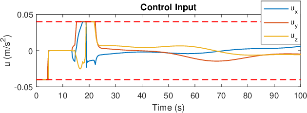
We then simulated trajectories under all three ZCBFs ($H$, $H^{\prime}$, $H_{o}$) in MATLAB¹¹ 1 All simulation code can be found at https://github.com/jbreeden-um/phd-code/tree/main/2021. The three simulated paths are shown in Fig. 2, and the corresponding control inputs are shown in Figs. 3-5. All three trajectories in Fig. 2 remained safe and generally followed similar paths around the obstacle. However, the control input only stayed within the designated control set in Figs. 3-4. For the trajectory under $H_{o}(x)$, the QP in (28) became infeasible at $t=14$ (see Fig. 5), so we had to expand the control set $U$ to compute a control input satisfying the safety constraint in (4). Thus, the proposed methods always yield trajectories that are safe in the presence of control input constraints, whereas earlier methods might not.

Additionally, note that the lines for $u_{x},u_{z}$ for $t\in[15,25]$ are slightly closer to the horizontal axis in Fig. 4 than in Fig. 3. This occurred because $H^{\prime}$ only makes use of $u\in U^{\prime}\subset U$ even though the QP was calculated over the complete control set $U$.

Next, we consider a spacecraft avoiding an object more complicated than a sphere, in this case an asteroid, but still in weak gravity, with gravity modeled by spherical harmonics [16]. If the asteroid is convex, one could simply use $h_{a}(x)$ as the constraint function, setting $r_{s}$ as the instantaneous closest point. However, if the asteroid is nonconvex (as in this example), the spacecraft could obtain a large velocity with respect to a point other than the closest point, so that strategy is no longer sufficient. Instead, we consider a discrete point-cloud model of the entire asteroid. The simplest response is to construct a ZCBF for every point in the model, similar to [17], though this could be computationally demanding. The result in [15, Thm. 3] allows us to to reduce the number of constraints to only those constraints that could be violated within some finite time horizon $\Delta t>0$ to reduce complexity. For this case study, we chose asteroid 433 Eros. The point cloud is a shape model of Eros with $N=7790$ plates [18], and gravity $f_{\mu}$ modeled in [19]. We construct a ZCBF with the form of $H^{\prime}(x)$ for every point, yielding $\{H_{i}^{\prime}(x)\}_{i=1}^{N}$. The trajectory, control inputs, and CBF values for the asteroid simulation are shown in Figs. 6-8 and a video of the scenario can be found at https://youtu.be/JKj3PUrYnEg. As expected, the trajectory is always safe and $u$ satisfies the input constraints. Since the spacecraft generally moves tangentially to the asteroid, $H$ is only slightly larger than $h_{a}$ for most of the simulation.

References

- [1] P. Wieland and F. Allgöwer, “Constructive safety using control barrier functions,” IFAC Proceedings Volumes, vol. 40, no. 12, pp. 462 – 467, 2007, 7th IFAC Symposium on Nonlinear Control Systems.
- [2] A. D. Ames, X. Xu, J. W. Grizzle, and P. Tabuada, “Control barrier function based quadratic programs for safety critical systems,” IEEE Trans. on Automatic Control, vol. 62, no. 8, pp. 3861–3876, Aug 2017.
- [3] L. Wang, A. D. Ames, and M. Egerstedt, “Safety barrier certificates for collisions-free multirobot systems,” IEEE Trans. on Robotics, vol. 33, no. 3, pp. 661–674, 2017.
- [4] L. Doeser, P. Nilsson, A. D. Ames, and R. M. Murray, “Invariant sets for integrators and quadrotor obstacle avoidance,” in 2020 American Control Conference, 2020, pp. 3814–3821.
- [5] J. Breeden and D. Panagou, “Quadratic programs for high relative degree spatial constraints and spatiotemporal specifications with spacecraft applications,” in 2020 59th IEEE Conference on Decision and Control, 2020, pp. 1496–1502.
- [6] T. Gurriet, M. Mote, A. D. Ames, and E. Feron, “An online approach to active set invariance,” in 2018 IEEE Conference on Decision and Control, 2018, pp. 3592–3599.
- [7] S. Hsu, X. Xu, and A. D. Ames, “Control barrier function based quadratic programs with application to bipedal robotic walking,” in 2015 American Control Conference, July 2015, pp. 4542–4548.
- [8] Q. Nguyen and K. Sreenath, “Exponential control barrier functions for enforcing high relative-degree safety-critical constraints,” in 2016 American Control Conference, July 2016, pp. 322–328.
- [9] W. Xiao and C. Belta, “Control barrier functions for systems with high relative degree,” in 2019 IEEE 58th Conference on Decision and Control, 2019, pp. 474–479.
- [10] X. Xu, “Constrained control of input–output linearizable systems using control sharing barrier functions,” Automatica, vol. 87, pp. 195–201, 2018.
- [11] A. Singletary, P. Nilsson, T. Gurriet, and A. D. Ames, “Online active safety for robotic manipulators,” in 2019 IEEE/RSJ Conference on Intelligent Robots and Systems (IROS), 2019, pp. 173–178.
- [12] E. Squires, P. Pierpaoli, and M. Egerstedt, “Constructive barrier certificates with applications to fixed-wing aircraft collision avoidance,” in 2018 IEEE Conference on Control Technology and Applications, 2018, pp. 1656–1661.
- [13] L. Wang, A. D. Ames, and M. Egerstedt, “Multi-objective compositions for collision-free connectivity maintenance in teams of mobile robots,” in 2016 IEEE 55th Conference on Decision and Control, 2016, pp. 2659–2664.
- [14] F. Blanchini, “Set invariance in control,” Automatica, vol. 35, no. 11, pp. 1747 – 1767, 1999.
- [15] P. Glotfelter, J. Cortés, and M. Egerstedt, “Boolean composability of constraints and control synthesis for multi-robot systems via nonsmooth control barrier functions,” in 2018 IEEE Conference on Control Technology and Applications, 2018, pp. 897–902.
- [16] L. M. Healy, “Space flight dynamics and navigation,” August 2018, draft: August 26, 2018.
- [17] M. Rauscher, M. Kimmel, and S. Hirche, “Constrained robot control using control barrier functions,” in 2016 IEEE/RSJ Conference on Intelligent Robots and Systems, Oct 2016, pp. 279–285.
- [18] P. C. Thomas and B. T. Carcich, “Msi eros shape model,” Cornell University Center for Radiophysics and Space Research,” Shape model of Eros derived from MSI data, June 2011, eros_2001012_007790.tab. [Online]. Available: https://sbnarchive.psi.edu/pds3/near/NEAR˙A˙MSI˙5˙EROS˙SHAPE˙MODELS˙V1˙0/data/eros˙2001012˙007790.tab
- [19] M. Torrence, “Nlr393v3 grav potential coefficients,” Goddard Space Flight Center,” GRAVITY MODEL, August 2001, rss/n393coeff.tab. [Online]. Available: https://sbnarchive.psi.edu/pds3/near/NEAR˙A˙5˙COLLECTED˙MODELS˙V1˙0/data/rss/n393coeff.tab