Differentially Private Sparse Vectors with Low Error,
Optimal Space, and Fast AccessConference: Proceedings of the 2021 ACM SIGSAC Conference on Computer and Communications Security; November 15–19, 2021; Virtual Event, Republic of Korea.Proceedings of the 2021 ACM SIGSAC Conference on Computer and Communications Security (CCS ’21), November 15–19, 2021, Virtual Event, Republic of KoreaPrice: 15.00ISBN: 978-1-4503-8454-4/21/11DOI: 10.1145/3460120.3484735CCS: Security and privacy Privacy-preserving protocols
Abstract.
Representing a sparse histogram, or more generally a sparse vector, is a fundamental task in differential privacy. An ideal solution would use space close to information-theoretical lower bounds, have an error distribution that depends optimally on the desired privacy level, and allow fast random access to entries in the vector. However, existing approaches have only achieved two of these three goals.
In this paper we introduce the Approximate Laplace Projection (ALP) mechanism for approximating -sparse vectors. This mechanism is shown to simultaneously have information-theoretically optimal space (up to constant factors), fast access to vector entries, and error of the same magnitude as the Laplace-mechanism applied to dense vectors. A key new technique is a unary representation of small integers, which we show to be robust against “randomized response” noise. This representation is combined with hashing, in the spirit of Bloom filters, to obtain a space-efficient, differentially private representation.
Our theoretical performance bounds are complemented by simulations which show that the constant factors on the main performance parameters are quite small, suggesting practicality of the technique.
Keywords:
Algorithms, Differential Privacy, Sparse VectorPublication
The paper appears in Proceedings of the 28th ACM Conference on Computer and Communications Security, 2021.
https://doi.org/10.1145/3460120.3484735
1. Introduction
One of the fundamental results in differential privacy is that a histogram can be made differentially private by adding noise from the Laplace distribution to each entry of the histogram before it is released (Dwork et al. 2016). The expected magnitude of the noise on each histogram entry is , where is the privacy parameter, and this is known to be optimal (Hardt and Talwar 2010). In fact, there is a sense in which the Laplace mechanism is optimal (Koufogiannis et al. 2015). However, some histograms of interest are extremely sparse, and cannot be represented in explicit form. Consider, for example, a histogram of the number of HTTP requests to various servers. Already the IPv4 address space has over 4 billion addresses, and the number of unique, valid URLs have long exceeded , so it is clearly not feasible to create a histogram with a (noisy) counter for each possible value.
Korolova, Kenthapadi, Mishra, and Ntoulas (Korolova et al. 2009) showed that it is possible to achieve approximate differential privacy with space that depends only on the number of non-zero entries in the histogram. However, for -differential privacy the upper bound on the expected per-entry error becomes , which is significantly worse than the Laplace mechanism for small . Cormode, Procopiuc, Srivastava, and Tran (Cormode et al. 2012) showed how to achieve pure -differential privacy with expected per-entry error bounded by , where is the dimension of the histogram, i.e., the number of entries. While both these methods sacrifice accuracy they are very fast, allowing access to entries of the private histogram in constant time. If access time is not of concern, it is possible to combine small space with small per-entry error, as shown by Balcer and Vadhan (Balcer and Vadhan 2019). They achieve an error distribution that is comparable to the Laplace mechanism (up to constant factors) and space proportional to the sum of all histogram entries — but the time to access a single entry is , which is excessive for large datasets.
1.1. Our results
Our contribution is a mechanism that achieves optimal error and space (up to constant factors) with only a small increase in access time. The mechanism works for either approximate or pure differential privacy, with the former providing faster access time. Our main results are summarized in Theorem 1.1.
Theorem 1.1 (Informal Version of Theorems 5.10 and 5.11).
Let be a histogram with entries each bounded by some value where at most entries have non-zero values. Given privacy parameters and , there exists an -differentially private algorithm to represent using bits with per-entry error matching the Laplace mechanism up to constant factors. The access time is when and when .
Here we assume that . Otherwise the mechanism has an additional term of or bits in its space usage for pure and approximate differential privacy, respectively.
1.2. Techniques
On a high level, we treat “small” and “large” values of the histogram differently. Large values are handled by the thresholding technique developed in (Korolova et al. 2009; Cormode et al. 2012). For small entries, we represent them using a unary encoding as fixed-length bit strings. From (Korolova et al. 2009; Cormode et al. 2012) we know that their length is logarithmic in either (for -DP) or (for )-DP). Privacy is achieved by perturbing each bit using randomized response (Warner 1965). As it turns out, the unary encoding is redundant enough to allow accurate estimation even when the probability of flipping each bit is a constant bounded away from 1/2. In order to pack all unary representations into small space, we use hashing to randomize the position of each bit in the unary representation of a given entry. The access time is linear in the length of the bit representation, given constant time evaluation of the hash function. Interestingly, although hash collisions can lead to overestimates, they do not influence the error asymptotically.
We remark here that a direct application of randomized response does not give the desired error dependency, but we solve this issue with an initial scaling step that gives -differential privacy when combined with randomized response. Though the discussion above has been phrased in terms of histograms, which makes the comparison to earlier work easier, our techniques apply more generally to representing sparse real vectors, with privacy for neighboring datasets with bounded -distance.
1.3. Overview
In Section 2 we define differential privacy for vectors, discuss the Laplace mechanism, and provide probabilistic tools necessary for the analysis. In Section 3 we discuss related work on differentially private sparse histograms. In Section 4 we introduce the Approximate Laplace Projection (ALP) mechanism and analyze its theoretical guarantees. In Section 5 we improve space and access time using techniques from earlier work (Korolova et al. 2009; Cormode et al. 2012). In Section 6 we evaluate the performance of the ALP mechanism based on simulations. In Section 7 we present suggestions for practical applications. We conclude the paper by stating an open problem in Section 8.
2. Preliminaries
Problem Setup.
In this work, we consider -dimensional -sparse vectors of non-negative real values. We say that a vector is -sparse if it contains at most non-zero entries. We assume that . All entries are bounded from above by a value , i.e., . Here is the set of integers . We consider the problem of constructing an algorithm for releasing a differentially private representation of , i.e., . Note that does not itself need to be -sparse.
Utility Measures.
We use two measures for the utility of an algorithm . We define the per-entry error as for any . We define the maximum error as . We compare the utility of algorithms using the expected per-entry and maximum error and compare the tail probabilities of the per-entry error of our algorithm with the Laplace mechanism introduced below.
Differential Privacy.
Differential privacy is a constraint to limit privacy loss introduced by Dwork, McSherry, Nissim, and Smith (Dwork et al. 2016). We use definitions and results as presented by Dwork and Roth (Dwork and Roth 2014). Intuitively, a differentially private algorithm ensures that a slight change in the input does not significantly impact the probability of seeing any particular output. We measure the distance between inputs using their -distance. In this work, two vectors are neighbors iff their -distance is at most 1. That is for all neighboring vectors we have . We can now define differential privacy for neighboring vectors.
Definition 2.1 (Differential privacy (Dwork and Roth 2014, Def 2.4)).
Given and , a randomized algorithm is -differentially private if for all subsets of outputs and pairs of -sparse input vectors such that it holds that:
satisfies approximate differential privacy when and pure differential privacy when . In particular, a pure differentially private algorithm satisfies -differential privacy. The following properties of differential privacy are useful in this paper.
Lemma 2.2 (Post-processing (Dwork and Roth 2014, Proposition 2.1)).
Let be an -differentially private algorithm and let be any randomized mapping. Then is -differentially private.
Lemma 2.3 (Composition (Dwork and Roth 2014, Theorem 3.16)).
Let and be randomized algorithms such that is -differentially private and is -differentially private. Then the algorithm where is -differentially private.
Throughout this paper, we clamp the output of all algorithms to the interval . An estimate outside this interval is due to noise and clamping outputs cannot increase the error. It follows from Lemma 2.2 that clamping the output does not affect privacy. We clamp the output implicitly to simplify presentation.
Probabilistic Tools.
The Laplace Mechanism introduced by Dwork, McSherry, Nissim, and Smith (Dwork et al. 2016) satisfies pure differential privacy by adding noise calibrated to the -distance to each entry. For completeness, Algorithm 1 provides a formulation of the Laplace mechanism in the context of releasing an -differentially private representation of a sparse vector.
2 Release .
Here is the Laplace distribution with scale parameter . The PDF and CDF of the distribution are presented in Definitions 2.4 and 2.5 and the expected error and tail bound of the mechanism are shown in Propositions 2.6 and 2.7. The Laplace mechanism works well for vectors with low dimensionality and serves as a baseline for our work. However, it is impractical or even infeasible in the setting of -sparse vectors. The output vector is dense, and as such the space requirement scales linearly in the input dimensionality .
Definition 2.4.
The probability density function of the Laplace distribution centered around 0 with scale parameter is
Definition 2.5.
The cumulative distribution function of the Laplace distribution centered around 0 with scale parameter is:
Proposition 2.6 (Expected Error (Dwork and Roth 2014, Theorem 3.8)).
The expected per-entry and maximum error of the Laplace mechanism are and respectively.
Proposition 2.7 (Tail bound (Dwork and Roth 2014, Theorem 3.8)).
With probability at least we have:
Random rounding or stochastic rounding is used for rounding a real value probabilistically based on its fractional part. We define random rounding for any real as follows:
Lemma 2.8.
The expected error of random rounding is maximized when . For any we have:
Randomized response was first introduced by Warner (Warner 1965). The purpose of the mechanism is to achieve plausible deniability by changing one’s answer to some question with probability and answer truthfully with probability . We define randomized response for a boolean value as follows:
Universal Hashing.
A hash family is a collection of functions mapping keys from a universe to a range . A family is called universal, if each pair of different keys collides with probability at most , where the randomness is taken over the random choice of . A particularly efficient construction that uses bits and constant evaluation time is presented in (Dietzfelbinger et al. 1997).
Model of Computation.
We use the -bit word RAM model defined by Hagerup (Hagerup 1998) where . This model allows constant time memory access and basic operations on -bit words. As such, we can store a -sparse vector using bits with constant lookup time using a hash table. We assume that the privacy parameters and can be represented in a single word.
Negative Values.
In this paper, we consider vectors with non-negative real values, but the mechanism can be generalized for negative values using the following reduction. Let be a real valued -sparse vector. Construct from such that and . By construction both and are -sparse and the -distance between vectors is preserved. We can access elements in as . As such, any differentially private representation of and can be used as a differentially private representation of with at most twice the error.
3. Related work
Previous work on releasing differentially private sparse vectors primarily focused on the special case of discrete vectors in the context of releasing the histogram of a dataset.
| Algorithm | Space (bits) | Access time | Per-entry error | Maximum error |
|---|---|---|---|---|
| Dwork et al. (Dwork et al. 2016) | ||||
| Cormode et al. (Cormode et al. 2012) | ||||
| Balcer & Vadhan (Balcer and Vadhan 2019) | ||||
| Theorem 5.10 (this work) | ||||
| Korolova et al. (Korolova et al. 2009) | ||||
| Theorem 5.11 (this work) |
Korolova, Kenthapadi, Mishra, and Ntoulas (Korolova et al. 2009) first introduced an approximately differentially private mechanism for the release of a sparse histogram. A similar mechanism was later introduced independently by Bun, Nissim, and Stemmer (Bun et al. 2019) in another context. The mechanism adds noise to non-zero entries and removes those with a noisy value below a threshold . The threshold is chosen such that the probability of releasing an entry with true value is at most . The expected maximum error is . Since is usually chosen to be negligible in the input size, we assume that . As such, the expected maximum error is . We discuss the per-entry error below. Their mechanism is designed to satisfy differential privacy for discrete data. We extend their technique to real-valued data as part of Section 5, where we combine it with our mechanism.
Cormode, Procopiuc, Srivastava, and Tran (Cormode et al. 2012) introduced a differentially private mechanism in their work on range queries for sparse data. The mechanism adds noise to all entries and removes those with a noisy value below a threshold . Here the threshold is used to reduce the expected output size. The number of noisy entries above is with high probability. The construction time of a naive implementation of their technique scales linearly in . They improve on this by sampling from a binomial distribution to determine the number of zero entries to store. They show that their approach produces the same output distribution as a naive implementation that adds noise to every entry. Their mechanism works for real-valued data in a straightforward way.
Since the expected number of non-zero entries in the output is for both mechanisms above, their memory requirement is bits using a hash table. An entry is accessed in constant time. The expected per-entry error depends on the true value of the entry. If the noisy value is above the threshold with sufficiently high probability, the expected error is . However, this does not hold for entries that are likely removed. Consider for example an entry with a true value exactly at the threshold . This entry is removed for any negative noise added. As such the expected per-entry error is for worst-case input, which is and for the two mechanisms, respectively.
In their work on differential privacy on finite computers, Balcer and Vadhan (Balcer and Vadhan 2019) introduced several algorithms including some with similar utility as the mechanisms described above. Moreover, they provided a lower bound of for the expected per-entry error of any algorithm that always outputs a sparse histogram. (See (Balcer and Vadhan 2019, Theorem 7.2) for the precise technical statement.) Here is the number of rows in the dataset, i.e., the sum of all entries of the histogram. This lower bound means that an algorithm that always outputs a -sparse histogram cannot achieve expected per-entry error for all input. They bypass this bound by producing a compact representation of a dense histogram. Their representation has expected per-entry and maximum error of and , respectively. It requires bits and an entry is accessed in time . Note that their problem setup differs from ours in that each entry is bounded only by such that . That is, serves a similar purpose as does in our setup. We do not know how to extend their approach to our setup with real-valued input.
In light of the results achieved in previous work, our motivation is to design a mechanism that achieves three properties simultaneously: expected per-entry error for arbitrary input, fast access, and (asymptotically) optimal space. Previous approaches only achieved at most two of these properties simultaneously. Moreover, we want the per-entry error to match the tail bounds of the Laplace mechanism up to constant factors. We construct a compact representation of a dense vector to bypass the lower bound for sparse vectors by Balcer and Vadhan (Balcer and Vadhan 2019). The access time of our mechanism is and for pure and approximate differential privacy, respectively. Table 1 summarizes the results of previous work and our approach.
4. The ALP mechanism
In this section, we introduce the Approximate Laplace Projection (ALP) mechanism11 1 The name is chosen to indicate that the error distribution is approximately like the Laplace distribution, and that we project the sparse vector to a much lower-dimensional representation. It also celebrates the mountains, whose silhouette plays a role in a certain random walk considered in the analysis of the ALP mechanism. and give an upper bound on the expected per-entry error. The ALP mechanism consists of two algorithms. The first algorithm constructs a differentially private representation of a -sparse vector and the second estimates the value of an entry based on its representation.
4.1. A 1-differentially private algorithm
We start by considering the special case of and later generalize to all values of . Moreover, the mechanism works well only for entries bounded by a parameter . In general, this would mean that we had to set if we only were to use the ALP mechanism. However, in Section 5 we will discuss how to set smaller and still perform well for all entries.
In the first step of the projection algorithm, we scale every non-zero entry by a parameter of the algorithm and use random rounding to map each such entry to an integer. We then store the unary representation of these integers in a two-dimensional bit-array using a sequence of universal hash functions (Carter and Wegman 1979). We call this bit-array the embedding. Lastly, we apply randomized response on the embedding to achieve privacy. The pseudocode of the algorithm is given in Algorithm 2 and we discuss it next.
2 Construct by hashing the unary representations of such that:
3 Apply randomized response to each bit of such that .
4 Release and .

The th entry is the only non-zero entry.Visualization of ALP-projectionWe use $m$ bits to represent each entry. Since we are storing the value 5, we set the first 5 bits to 1.
Figure 1 shows an example of an embedding before applying randomized response. The input is a vector where the th entry is the only non-zero value. The result of evaluating for each hash function is shown in the table at the bottom and the bits representing the th entry in the bit-array are highlighted. In Step (1) of the algorithm, is scaled by and randomized rounding is applied to the scaled value. This results in . Using the hash functions, we represent this value in unary encoding by setting the first five bits to in Step (2), where the th bit is selected by evaluating the hash function on . The final three bits are unaffected by the entry. Finally, we apply randomized response in each cell of the bit-array. The bit-array after applying randomized response is not shown here, but we present it later in Figure 2. Both the bit-array and the hash functions are the differentially private representation of the input vector . We use this construction when estimating the value of later.
The algorithm takes three parameters , and . The parameters and are adjustable. We discuss these parameters later as part of the error analysis. In Section 6 we discuss how to select values for and . Throughout the paper we sometimes assume that is a constant and is a constant multiple of that is and . The parameter bounds the values stored in the embedding. We discuss as part of the error analysis as well.
Lemma 4.1.
Algorithm 2 satisfies 1-differential privacy.
Proof.
Let denote two neighboring vectors. We prove the lemma in several steps. First, the vectors differ only in their th entry. In this case, we start by assuming that only a single bit of is affected by changing to and that there are no hash collisions. We then allow them to differ in several bits and include hash collisions. Finally, we generalize to the case that they differ in more than one entry.
Assume that differs only in a single bit for and . Let denote the event that the affected bit is set to one after running the algorithm. Let be the parameter of the randomized response step and let . Then the probability of occurring with input is , where denotes the probability of the bit being one before the randomized response step. Similarly for we define . The minimum term is needed when is a multiple of such that . We find the difference in the probability of occurring for and as:
By symmetry, the absolute difference in probability for setting the bit to either zero or one is . Let be an arbitrary output of Algorithm 2. Since and agree on all but the th entry, the change in probability of outputting depends only on the affected bit. Let denote the event that the bit agrees with output . Then we find the ratio of probabilities of outputting as:
Here the second inequality follows from . From here it is easy to take hash collisions into account as follows: Let denote the probability of occurring after setting the th entry to zero. That is, we have and . The absolute difference in probability is still bounded such that . As such it still holds that:
Next, we remove the assumption that only a single bit is affected by composing probabilities. We provide the following inductive construction. Let be vectors that differ in the th entry such that exactly two bits are affected. We consider the case of and fix a vector with such that the differences affects exactly one bit each. Again, let be an arbitrary output of Algorithm 2. Applying the upper bound from above twice, we may bound the change in probabilities by:
which can be applied inductively if changing an entry affects more than two bits.
We are now ready to generalize to any vectors , i.e., where vectors may differ in more than a single position. Using the bound from above, we can bound the ratio of probabilities by:
The privacy loss is thus bounded by the -distance of the vectors for any output. Recall that the -distance is upper bounded by for two neighboring vectors. As such the algorithm is -differentially private as for any pair of neighboring vectors and and any subset of outputs we have:
∎
The following lemma summarizes the space complexity of storing the bit-array and the collection of hash functions.
Lemma 4.2.
The number of bits required to store and is
Proof.
By definition and as such bits are used to store . Each hash function uses bits for a total of bits to store . ∎
4.2. Estimating an entry
We now introduce the algorithm to estimate an entry based on the embedding from Algorithm 2. When accessing the th entry, we estimate the value of and multiply by to reverse the initial scaling of . The estimate of is chosen to maximize a partial sum. If multiple values maximize the sum we use their average.
Intuition.
The first bits representing the th entry are set to one before applying noise in Algorithm 2, cf. Figure 1. The last bits are zero, except if there are hash collisions. Some bits might be flipped due to randomized response, but we expect the majority of the first bits to be ones and the majority of the remaining bits to be zeros. As such the estimate of is based on prefixes maximizing the difference between ones and zeros. The pseudocode for the algorithm is given as Algorithm 3.
2 Let be the set of arguments maximizing . That is,
3 Let
4 Return .

The partial sum is maximized at indices 3 and 5.
The estimate is 4, while the true value was 5. Visualization of ALP1-estimationWe use $m$ hash functions to estimate the projected entry.
Figure 2 shows an example of Algorithm 3. The example is based on the embedding from Figure 1 after adding noise. The plot shows the value of for all candidate estimates. This sum is maximized at positions and . This is visualized as the global peaks in the plot. The estimate is the average of those positions.
Lemma 4.3.
The evaluation time of Algorithm 3 is .
Proof.
We can compute all partial sums by evaluating each bit once using dynamic programming. As such the evaluation time is with . We have when . ∎
We now analyze the per-entry error of Algorithm 3. We first analyze the expected error based on the parameters of the algorithm. The results are presented in Lemma 4.8. In Lemmas 4.9 and 4.10 we bound the tail distribution of the per-entry error of the algorithm.
Lemma 4.4.
The expected per-entry error of Algorithm 3 is bounded by for entries with a value of at most .
Proof.
It is clear that the error of the th entry is times the difference between and . The expected difference is bounded by:
The last inequality follows from Lemma 2.8. ∎
We find an upper bound on by analyzing simple random walks. A simple random walk is a stochastic process such that and , where are independent and identically distributed random variables with and .
Lemma 4.5.
Let be a simple random walk with . At any step the probability that there exists a later step such that is .
Proof.
It follows directly from Theorem 1 by Alm (Alm 2002). ∎
For our analysis, we are concerned with the maximum such that . For an infinite random walk where such an exists with probability .
Lemma 4.6.
Let be a simple random walk with . The expected last non-negative step of is: .
Proof.
We use Lemma 4.5 to find the probability that is the unique maximum in as follows:
The last non-negative step must have value exactly zero and as such must be at an even numbered step. The probability that step is the last non-negative is:
We are now ready to find the expected last non-negative step of an infinite simple random walk as:
The last equality follows from the identity . See Appendix A for a proof of this identity. ∎
We are now ready to bound . We consider entries with value at most , i.e., .
Lemma 4.7.
Let and . Then the expected value of is bounded such that
Proof.
Recall the definition of from Algorithm 3. Let denote an element furthest from that is for all . It it clearly sufficient to consider for the proof since . We first consider the case of . It follows from the definition of as a maximum that . As such at least half the bits must be zero, that is they were flipped by randomized response in Step (3) of Algorithm 2. As such the length of the longest interval ending at bit where at least half the bits were flipped is an upper bound on the value of . The expected size of said interval is bounded by the expected last non-negative step of a simple random walk with . It follows from Lemma 4.6 that:
We can use a similar argument when to show that at least half the bits in must be since is a maximum. In this case we have to consider the possibility of hash collisions. Each hash function maps to and at most entries result in a hash collision. The probability of a hash collision is at most using a union bound. As such for we have . We let such that by Lemma 4.6 and the calculation above. We isolate to find:
Note that holds due to the requirement of Algorithm 2. By conditional expectation, we may upper bound the total expected error by
| (1) |
∎
As such we can bound the expected per-entry error for entries with a true value of at most by a function of the parameters and . In Section 6 we discuss the choice of these parameters based on the upper bond and experiments. For any fixed values of and we have:
Lemma 4.8.
Let and . Then the expected per-entry error of Algorithm 3 is .
Proof.
where . Entries above have an additional error of up to , since and are represented identically in the embedding by Algorithm 2. Since and are constants we have:
∎
Next, we bound the tail probabilities for the per-entry error of the mechanism. We bound the error of the estimate , which implies bounds on the error of the mechanism.
Lemma 4.9.
Let and . Let and . Then for Algorithm 3 we have:
Proof.
Let be a simple random walk. We find an upper bound on the probability that the position of the last non-negative step in is at least :
where the first inequality follows from when (Elkies 2013). The last inequality follows from . As discussed in the proof of Lemma 4.7, the expectation of can be bounded by two random walks each with at most . ∎
Lemma 4.10.
Let , and . With probability at least for Algorithm 3 we have:
Proof.
Up to constant factors, the tail probabilities of our mechanism are similar to the properties of the Laplace mechanism summarized in Proposition 2.7. The probabilities depend on the parameters of the mechanism. In Section 6 we fix the parameters and evaluate the error in practice. We summarize the tail probabilities for in Lemma 4.11.
Lemma 4.11.
4.3. Generalization to -differential privacy
We now generalize the ALP mechanism from -differential privacy to satisfying -differential privacy. A natural approach is to use a function of as the parameter for randomized response in Algorithm 2. The projection algorithm is -differentially private if we remove the scaling step and set . However, the expected per-entry error would be bounded by by Equation 4.2 (without considering hash collisions), which is as large as for small values of . Other approaches modifying the value of have a similar expectation.
In the following, we use a simple pre-processing and post-processing step to achieve optimal error. The idea is to scale the input vector as well as the parameter by before running Algorithm 2. We scale back the estimates from Algorithm 3 by . These generalizations are given as Algorithm 4 and Algorithm 5, respectively.
2 Let .
3 Release and .
2 Return .
Lemma 4.12.
Algorithm 4 satisfies -differential privacy.
Proof.
It follows from the proof of Lemma 4.1 that for any subset of outputs we have . As such for any pair of neighboring vectors and we have:
∎
Lemma 4.13.
Let and . The output of Algorithm 4 can be stored using bits.
Proof.
It follows from Lemma 4.2 that the output can be stored using bits. Recall that we assume , i.e., . ∎
Lemma 4.14.
Let and . Then the expected per-entry error of Algorithm 5 is and the evaluation time is .
Proof.
Lemma 4.15.
Proof.
It follows directly from Lemma 4.11. ∎
We are now ready to state the following theorem which summarizes the properties of the ALP mechanism.
Theorem 4.16.
Let , . Then there exist an algorithm where the expected per-entry error is for all entries, the access time is , and the space usage is bits.
The space usage and access time of the mechanism both scale linearly with the parameter . As such the mechanism performs well only for small values of . However, in many contexts scales with the input size. One example is a histogram, where is the number of rows in the underlying dataset. Next, we show how to handle such cases.
5. Combined data structure
In this section, we combine the ALP mechanism with techniques from previous work to improve space requirements and access time. As shown in Theorem 4.16 the ALP mechanism performs well when all entries are bounded by a small value. The per-entry error is low only for entries bounded by but the space requirements and access time scale linearly with . Some of the algorithms from previous work perform well for large entries but have large per-entry error for small values. The idea of this section is to combine the ALP mechanism with such an algorithm to construct a composite data structure that performs well for both small and large entries.
To handle large values, we use the thresholding technique from Cormode et al. (Cormode et al. 2012). It adds noise to each entry, but only stores entries above a threshold. The pseudocode of the algorithm is given as Algorithm 6.
2 Truncate entries below :
Lemma 5.1.
Algorithm 6 satisfies -differential privacy.
Proof.
The algorithm is equivalent to the Laplace mechanism followed by post-processing. The Laplace mechanism satisfies -differential privacy, and privacy is preserved under post-processing as stated by Lemma 2.2. ∎
Lemma 5.2.
Let . Then the output of Algorithm 6 is -sparse with high probability.
Proof.
Using Definition 2.5 we find that the probability of storing a zero entry is:
By linearity of expectation, the expected number of stored true zero entries is at most one, and as such the vector is -sparse with high probability. ∎
As discussed in Section 3, the expected per-entry error of Algorithm 6 is for worst-case input. We combine the algorithm with the ALP mechanism from the previous section to achieve expected per-entry error for any input. We use the threshold parameter as value for parameter in Algorithm 4. The algorithm is presented in Algorithm 7.
2 Let .
3 Let
4 Return , and .
Lemma 5.3.
Algorithm 7 satisfies -differential privacy.
Proof.
The two parts of the algorithm are independent as there is no shared randomness. The first part of the algorithm satisfies -differential privacy by Lemma 5.1 and the second part satisfies -differential privacy by Lemma 4.12. As such it follows directly from composition (Lemma 2.3) that Algorithm 7 satisfies -differential privacy. ∎
Lemma 5.4.
Let , , . Then the output of Algorithm 7 is stored using bits with high probability.
Proof.
To estimate an entry, we access when a value is stored for the entry and the ALP embedding otherwise. This algorithm is presented in Algorithm 8.
Lemma 5.5.
Proof.
The evaluation time follows from Lemma 4.14. That is, the evaluation time is .
The error depends on both parts of the algorithm. The expected per-entry error for the th entry is when by Lemma 4.14. That is, when is less than in Algorithm 6. When the error is the absolute value of . That is, we can analyze it using conditional probability and the probability density function of the Laplace distribution from Definition 2.4.
The expected maximum error of Algorithm 6 is and the output of the Algorithm 5 is at most . Since the expected maximum error is . ∎
5.1. Removing the dependency on dimension
To make access time independent of the dimension , we can turn to approximate differential privacy. This allows us to use a smaller threshold in the initial thresholding approach, which in turn results in smaller values for in the ALP mechanism.
The following algorithm is similar to that introduced by Korolova et al. (Korolova et al. 2009), which we discussed in Section 3. It adds noise to non-zero entries only, and uses a threshold to satisfy approximate differential privacy. Our algorithm differs from the work of Korolova et al. by using a random rounding step. This step is not needed in a discrete setting, where at most a single zero-valued entry is changed to a non-zero entry for neighboring vectors. However, in the real-valued context, several zero entries can change.
2 Let for all non-zero entries, where .
3 Let .
4 Truncate entries below :
5 Return .
Lemma 5.6.
Algorithm 9 satisfies -differential privacy.
Proof.
Let and be neighboring vectors. We consider two additional vectors and such that:
The vectors are constructed such that and can only differ for entries at most in both vectors. The same holds for and . Additionally, the -distance is still at most between any pair of vectors.
We find the probability of outputting anything for an entry less than or equal to as:
Since and only differ for entries less than or equal to we have for any subset of outputs :
The inequality holds in both directions and for the pair of and as well.
By definition and only differ for entries of at least . As such we can ignore the random rounding step and we have:
Using the inequalities above we have:
∎
Lemma 5.7.
Let . Then the expected maximum error of Algorithm 9 is .
Proof.
The expected maximum error added by the Laplace noise is , since we add noise to at most entries. By removing entries we add error of up to . As such the expected maximum error for worst-case input is:
∎
Lemma 5.8.
Lemma 5.9.
Let , , and . Then the memory requirement of combining Algorithm 9 and the ALP mechanism is .
Proof.
We are now ready to summarize our results for both pure and approximate differential privacy.
Theorem 5.10.
Let , , and . Then there exists an -differentially private algorithm with expected per-entry error, expected maximum error, access time of , and space usage of with high probability.
Theorem 5.11.
Let , , and . Then there exist an -differentially private algorithm with expected per-entry error, expected maximum error, access time of , and space usage of .
6. Experiments
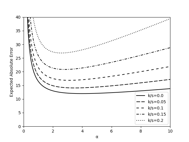
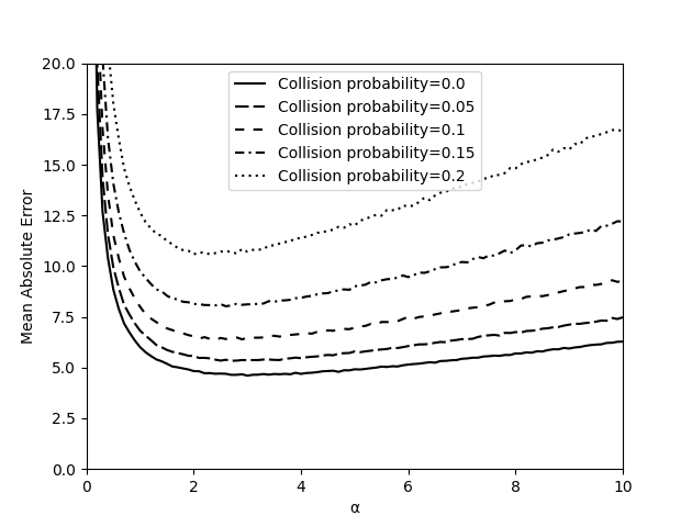

Note that the y-axes for the plots use different scales.Plot of the upper bound and observed per-entry errorThe plots show the expected per-entry error for varying parameters of $\alpha$ and $k/s$. The plots follow similar trajectories, but the observed error is approximately half the theoretical upper bound.
In this section, we discuss the per-entry error of ALP1-estimator (Algorithm 3) in practice. Let . By Lemma 4.4 and 4.7 the expected per-entry error of ALP1-estimator is upper bounded by:
Figure 3(a) shows the upper bound for varying values of and . Recall that is a bound on the probability of a hash collision. We see that the effect of hash collisions on the error increases for large values of , as each bit in the embedding is more significant. We discuss how the upper bound compares to practice next.
Experimental Setup.
We designed experiments to evaluate the effect of the adjustable parameters and on the expected per-entry error of ALP1-estimator. The experiments were performed on artificial data. For our setup, we set parameter and chose a true value uniformly at random in the interval . We run only on artificial data, as uniform data does not benefit the algorithm, and we can easily simulate worst-case conditions for hash collisions. We simulate running the ALP1-projection algorithm by computing , simulating hash collisions, and applying randomized response. The probability for hash collisions is fixed in each experiment and the same probability is used for all bits. This simulates worst-case input in which all other non-zero entries have a true value of at least . We increment by steps of in the interval and the probability of a hash collision by in the interval . The probability of serves only as a baseline, as it is not achievable in practice for . The experiment was repeated times for every data point.
Figure 3(b) shows plots of the mean absolute error of the experiments. As is increased, the error drops off at first and slowly climbs. The estimates of are more accurate for large values of . However, any inaccuracy is more significant, as is scaled back by a larger value. The error from the random rounding step also increases with . The plots of the upper bound and observed error follow similar trajectories. However, the upper bound is approximately twice as large for most parameters.
Fixed Parameters.
The experiments show how different values of and affect the expected per-entry error. However, the parameters also determine constant factors for space usage and access time. The space requirements scale linearly in and the access time is inversely proportional to . As such, the optimal parameter choice depends on the use case due to space, access time, and error trade-offs.
To evaluate the error distribution of the ALP1-estimator algorithm we fixed the parameters of an experiment. We set and the hash collision probability to . We repeated the experiment times.
The error distribution is shown in Figure 3(c). The mean absolute error of the experiment is and the standard deviation is . Plugging in the parameters in Lemma 4.11, with probability at least 0.9 the error is at most
The error of the observed th percentile is , which is shown in Figure 3(c) using vertical lines. Again, this shows that the upper bounds are pessimistic.
For comparison, the plots include the Laplace distribution with scale parameters and . Note that the Laplace distribution with parameter is optimal for the privacy budget. The standard deviation of the distribution with scale is and as such the mean absolute error is similar to the ALP mechanism.
The distribution is slightly off-center, and the mean error is . This is expected due to hash collisions. The effect of hash collisions is also apparent for the largest observed errors. The lowest observed error was , while the highest was . There is a clear trade-off between space usage and per-entry error. We reran the experiment with hash collision probability using the same value for . The error improved for all the metrics mentioned above. The mean absolute error is , the standard deviation is , the mean error is , the th percentile is , and the largest observed error is .
7. Suggestions to Practitioners
The ALP mechanism introduced in this paper combines the best of three worlds: It has low error similar to the Laplace mechanism, produces compact representations using asymptotically optimal space, and has an access time that scales only with .
In an application that wants to make use of differentially private histograms/vectors, one first has to get an overview of the assumed properties of the data before making a choice on which approach to use. If is small or the data is assumed to be dense, the Laplace mechanism will offer the best performance. If the data is sparse and the dimension is large, the analyst must know which error guarantee she wishes to achieve, and which access time is feasible in the setting where the application is deployed. If a larger error is acceptable for “small” entries or access time is crucial, just applying the thresholding technique (Korolova et al. 2009; Cormode et al. 2012) is the better choice. Otherwise, if small error is paramount or an access time of is sufficient, the ALP mechanism will provide the best solution.
Variants.
We assume in this paper that is a known bound on the sparsity of the input data. However, in some applications the value of itself is private. Here we briefly discuss approaches in such settings. We use the value of to select the size of the embedding, such that the probability of hash collisions is sufficiently small. When is not known we can still bound the probability of hash collisions.
If the input is a histogram the sparsity differs by at most for neighboring datasets. As such we can use a fraction of the privacy budget to estimate the sparsity. Note that this is not possible for vectors, as the difference in sparsity can be as large as for neighboring datasets.
If is known then we have for the scaled input. We can bound the probability of hash collisions by a constant when the size of the embedding is bits. If is unknown we can estimate it using a fraction of the privacy budget. Note that the space differs from the -sparse setting, and remains bits when applying the thresholding techniques.
An implementation of a variant of the ALP mechanism is available as part of the open source project OpenDP (https://opendp.org/) in the repository https://github.com/opendp/opendp.
8. Open problems
The main open problem that we leave is if it is possible to achieve similar space and error with constant time access. We know of a way (based on the count-min sketch) to achieve optimal expected error with constant time access and space within a logarithmic factor of optimal. However, this method does not have strong tail bounds on the error.
Acknowledgements.
We thank the anonymous reviewers for their detailed suggestions that helped improve the paper. Christian Janos Lebeda and Rasmus Pagh are affiliated with Basic Algorithms Research Copenhagen (BARC), supported by the VILLUM Foundation grant 16582.References
- (1)
- Alm (2002) Sven Erick Alm. 2002. Simple random walk. Unpublished manuscript (2002). http://www2.math.uu.se/˜sea/kurser/stokprocmn1/slumpvandring_eng.pdf
- Balcer and Vadhan (2019) Victor Balcer and Salil P. Vadhan. 2019. Differential Privacy on Finite Computers. J. Priv. Confidentiality 9, 2 (2019).
- Bun et al. (2019) Mark Bun, Kobbi Nissim, and Uri Stemmer. 2019. Simultaneous Private Learning of Multiple Concepts. J. Mach. Learn. Res. 20 (2019), 94:1–94:34.
- Carter and Wegman (1979) Larry Carter and Mark N. Wegman. 1979. Universal Classes of Hash Functions. J. Comput. Syst. Sci. 18, 2 (1979), 143–154.
- Cormode et al. (2012) Graham Cormode, Cecilia M. Procopiuc, Divesh Srivastava, and Thanh T. L. Tran. 2012. Differentially private summaries for sparse data. In ICDT. ACM, 299–311.
- Dietzfelbinger et al. (1997) Martin Dietzfelbinger, Torben Hagerup, Jyrki Katajainen, and Martti Penttonen. 1997. A Reliable Randomized Algorithm for the Closest-Pair Problem. J. Algorithms 25, 1 (1997), 19–51.
- Dwork et al. (2016) Cynthia Dwork, Frank McSherry, Kobbi Nissim, and Adam D. Smith. 2016. Calibrating Noise to Sensitivity in Private Data Analysis. J. Priv. Confidentiality 7, 3 (2016), 17–51.
- Dwork and Roth (2014) Cynthia Dwork and Aaron Roth. 2014. The Algorithmic Foundations of Differential Privacy. Found. Trends Theor. Comput. Sci. 9, 3-4 (2014), 211–407.
- Elkies (2013) Noam D. Elkies. 2013. Upper limit on the central binomial coefficient. https://mathoverflow.net/questions/133732/upper-limit-on-the-central-binomial-coefficient. [Online; accessed 15-September-2021].
- Graham et al. (1994) Ronald L. Graham, Donald E. Knuth, and Oren Patashnik. 1994. Concrete Mathematics: A Foundation for Computer Science, 2nd Ed. Addison-Wesley.
- Hagerup (1998) Torben Hagerup. 1998. Sorting and Searching on the Word RAM. In STACS (Lecture Notes in Computer Science, Vol. 1373). Springer, 366–398.
- Hardt and Talwar (2010) Moritz Hardt and Kunal Talwar. 2010. On the geometry of differential privacy. In STOC. ACM, 705–714.
- Korolova et al. (2009) Aleksandra Korolova, Krishnaram Kenthapadi, Nina Mishra, and Alexandros Ntoulas. 2009. Releasing search queries and clicks privately. In WWW. ACM, 171–180.
- Koufogiannis et al. (2015) Fragkiskos Koufogiannis, Shuo Han, and George J. Pappas. 2015. Optimality of the Laplace Mechanism in Differential Privacy. CoRR abs/1504.00065 (2015).
- Warner (1965) Stanley L Warner. 1965. Randomized response: A survey technique for eliminating evasive answer bias. J. Amer. Statist. Assoc. 60, 309 (1965), 63–69.
Appendix A Closed-form proof of Lemma 4.6
Here we provide a closed-form expression used in the proof of Lemma 4.6.
In the proof, we will make use of general binomial coefficient((Graham et al. 1994, Equation 5.1)):
and the binomial theorem ((Graham et al. 1994, Equation 5.12)):
Starting from an infinite series with , we simplify as follows:
Let and . Then we have:
Finally, let and let . This gives us the closed-form expression: