Robust deep hedging
Abstract
We study pricing and hedging under parameter uncertainty for a class of Markov processes which we call generalized affine processes and which includes the Black-Scholes model as well as the constant elasticity of variance (CEV) model as special cases. Based on a general dynamic programming principle, we are able to link the associated nonlinear expectation to a variational form of the Kolmogorov equation which opens the door for fast numerical pricing in the robust framework.
The main novelty of the paper is that we propose a deep hedging approach which efficiently solves the hedging problem under parameter uncertainty. We numerically evaluate this method on simulated and real data and show that the robust deep hedging outperforms existing hedging approaches, in particular in highly volatile periods.
Keywords: affine processes, Knightian uncertainty, Kolmogorov equation, deep learning, robust hedging
JEL classification: C02, C45, G13
1Department of Quantitative Finance,
Institute for Economic Research, University of Freiburg,
Rempartstr. 16,
79098 Freiburg, Germany.
2Department of Mathematical Stochastics, Mathematical Institute,
University of Freiburg, Ernst-Zermelo-Str. 1, 79104 Freiburg, Germany.
3NTU Singapore, Division of Mathematical Sciences,
21 Nanyang Link, Singapore 637371
1 Introduction
Uncertainty, as coined by Frank Knight, refers to the case where a number of models (technically: probability measures) are available and one is not able to distinguish between them. This applies for example to the prediction of the evolution of a stock in the future. Even if we have a reliable and rich source of historic information, predicting the future evolution, the future variance or even the whole future distribution is highly complicated. On the one side, this is due to the classical estimation problem: estimated parameters allow for confidence intervals which need to be taken into account for the prediction. On the other side, in particular in financial markets, changes in the underlying dynamics are rather the rule than the exception and additional uncertainty and model risk come into effect, resulting in a widening of confidence intervals. For pricing, one can efficiently rely on the calibration to option surfaces with all its difficulties. For hedging, when one wants to incorporate the performance under the objective measure and not under the risk-neutral one, this becomes much more challenging.
Our paper addresses exactly this setting and suggests a deep learning approach for hedging under parameter uncertainty. The basis for our work is the recently developed class of affine processes under parameter uncertainty, see Fadina et al. 2019, which we simply call nonlinear affine processes, referring to the associated nonlinear expectation arising from the pricing problem under uncertainty in this class. We extend this approach to those Markovian processes which satisfy
| (1.1) |
where we allow for parameter uncertainty in all the parameters , and . We develop the theory for this class of processes which we call nonlinear generalized affine (NGA) processes. The robust pricing problem is solved by utilizing a general dynamic programming principle and establishing the nonlinear Kolmogorov equation, which opens the door for fast (and well-known) numerical approaches. In order to solve the hedging problem under parameter uncertainty, we rely on a deep learning approach. To the best of our knowledge, this is the first attempt of this kind.
We numerically evaluate this method first on simulated data and show that the robust deep hedging outperforms existing hedging approaches when parameter uncertainty is present. For a realistic data application, we consider the COVID-19 period. In this period, stock markets experienced unexpectedly high volatility and variation in the price paths, which poses a huge challenge to classical hedging approaches. When applying robust methods, the first challenge is to find reliable estimates for the parameter intervals specifying the uncertainty in the considered model class. We propose a sliding-window maximum-likelihood estimation approach for this whose maximal and minimal parameter estimates lead to the targeted intervals. With this uncertainty specification at hand, we are able to show that in the considered data examples the robust deep hedging approach leads to a remarkably smaller hedging error in comparison to classical hedging strategies.
Our paper relates to a rich stream of literature motivated by parameter uncertainty, dating back to Avellaneda et al. 1995, Wilmott and Oztukel 1998, and Fouque and Ren 2014. More recent contributions are Cohen and Tegnér 2017, Barnett et al. 2020, Aksamit et al. 2020, Cheridito et al. 2017, Akthari et al. 2020. In the context of option pricing and efficient hedging, Bouchard et al. 2015, Hou and Obłój 2018 developed approaches respecting an ambiguity set of possible underlying probability measures and Acciaio et al. 2016, Beiglböck et al. 2013, Cox and Obłój 2011, Dolinsky and Soner 2014, Hobson 1998, Lütkebohmert and Sester 2019, Nadtochiy and Obłój 2017, Neufeld and Sester 2021b introduced approaches to entirely model-free option pricing and to model-free super-replication.
Further, our paper contributes to the recent literature on deep learning approaches in hedging, starting from the seminal work Buehler et al. 2019 and followed by Gümbel and Schmidt 2020, Cuchiero et al. 2020, Cao et al. 2021, Carbonneau 2021, Carbonneau and Godin 2021, Chen and Wan 2021, Eckstein et al. 2021, Gierjatowicz et al. 2020, Horváth et al. 2021, Neufeld and Sester 2021a, amongst many others (see also Ruf and Wang 2020 for a review).
The remainder of the paper is organized as follows: In Section 2 we introduce the theoretical basis for NGA processes. In Section 3 we introduce the robust hedging approach, illustrated with simulated examples, while in Section 4 we apply robust hedging to real data. Section 5 concludes and the appendix contains some proofs.
2 Generalized affine processes under parameter uncertainty
In this section we extend the notion of affine diffusions under parameter uncertainty to a more general setting. To this end, consider a state space which is either or . We start with the setting without parameter uncertainty.
A generalized affine diffusion is a continuous semimartingale which is a unique strong solution of the stochastic differential equation (SDE)
| (2.1) |
with suitably chosen , , and initial value . Here, denotes a standard Brownian motion. If we choose we obtain the well-known special case of a (continuous) affine process.
In Proposition A.2 in the appendix we utilize the classical existence result of Engelbert and Schmidt (Engelbert and Schmidt 1985a, Engelbert and Schmidt 1985b) to show that a generalized affine diffusion exists on a proper state space.
Fix a time horizon and consider as the canonical space of continuous one-dimensional paths. Denote by the Borel--algebra on . Let be the canonical process for and and denote by the filtration generated by .
Let be the set of all probability measures on . A probability measure is called a semimartingale law for the process if there exists a process with continuous paths of (locally) finite variation -a.s. and a continuous local -martingale with such that Intuitively, this describes the setting when is a continuous semimartingale under which is given as a sum of the integrated drift process and a local martingale .
A continuous semimartingale is said to admit absolutely continuous characteristics with if there exist predictable processes and such that11 1 Note that does not depend on as the quadratic variation is a path property. We therefore write and .
| (2.2) |
In the case that a continuous semimartingale possesses absolutely continuous characteristics, we can directly consider the drift (instead of the integrated drift).
2.1 Parameter uncertainty
Next, we introduce parameter uncertainty in the spirit of Frank Knight. Recall that a generalized affine diffusion is characterized by the five parameters and . The targeted uncertainty we are interested in can be described as follows: instead of assuming the parameter to be known exactly, we introduce an interval and consider each value in the interval equally likely. Taking into account this parameter uncertainty leads to a nonlinear setting, which we introduce now.
Denote the considered parameter intervals by and with , and by . Denote by the parameter set.
To transport this parameter uncertainty to stochastic processes we have to be more careful. In the Markovian setting we consider here, the evolution of the process may depend on the current state of the process. In this regard, we introduce the associated intervals
| (2.3) |
for , where which describe the possible diffusive behaviour of the process given it is in state .
Remark 2.1 (On the role of the state space)
In the classical one-dimensional affine setting, the state space already defines if the affine process is of Cox-Ingersoll-Ross type (when the state space is or ) or of Vasiček-type. This is no longer the case when parameter uncertainty is introduced. Indeed, in Fadina et al. 2019, the non-linear Vasiček-CIR model was introduced which has as state space and intuitively is able to capture both sorts of dynamics. In interest rate markets, where negative rates have been neglected for a long time, such an approach efficiently avoids the model risk by the necessity to choose between the state space and . In the non-linear setting considered here, this leads to the use of in the definition of . This ensures non-negativity of the quadratic variation when but does not restrict unnecessarily the dynamics of the generalized affine process.
The description of the generalized affine process under parameter uncertainty is now intuitively given by all those probability laws describing a diffusion where the drift and the volatility always stay in the intervals and considered at . This means, that we consider all continuous semimartingales whose characteristics stay in the parameter uncertainty bounds.
More precisely, we introduce the following notion22 2 The name (nonlinear) generalized affine process and the setting of a NGA is inspired by the master thesis Denk 2021.: a nonlinear generalized affine process (NGA) starting in at time is the family of all absolutely continuous semimartingale laws , such that for each giving rise to the differential characteristics we have
| (2.4) |
-almost surely on and . We call generalized affine dominated by on or simply GA-dominated by . Note that non-negativity of the quadratic variation is ensured by using in the definition of in Equation (2.3)
2.2 Robust pricing of derivatives
In order to study derivative prices under parameter uncertainty, we consider an European claim with maturity and payoff . Here, is an integrable function .
Since in our robust setting we do not have a single probability measure at hand, but a family of measures which we treat equally likely, a natural candidate for pricing is the worst-case price: the price which dominates all prices computed under the probability measures we consider.
In this regard, define the value function by
Analogously one can define a lower bound of possible prices , which, due to the relation , can be studied with identical methods. We therefore focus on the upper bound.
A central tool for establishing a nonlinear Kolmogorov equation and therefore the tractability of the setting is the dynamic programming principle. Intuitively it states that if we consider a stopping time between and and compute the price (the value function) at that stopping time and take expectations of this random quantity, we obtain the value function at time . Thus, the value can not be improved by however skilled stopping.
Proposition 2.2
Consider a nonlinear generalized affine process with state space and a stopping time on For any , we have
| (2.5) |
The proof of this result follows similarly to the proof of the dynamic programming principle in Fadina et al. 2019 which is based on Theorem 2.1 in El Karoui and Tan 2013. The necessary measurability and stability conditions which are proved for the affine case in Lemma 1 and 2 of Fadina et al. 2019 can be shown similarly for the generalized affine case.
2.3 The nonlinear Kolmogorov equation
Note that the computation of the value function according to Equation (2.5), or the robust upper price of a derivative is not as easily accessible by Monte-Carlo estimation as in the classical case. Indeed, as is clear form Equation (2.5), it is not sufficient to simulate different paths under different distributions but we need to obtain Monte-Carlo estimates of expectations with a fixed probability measure and then need to find the supremum of these expectations. If no monotonicity can be exploited, this will be difficult to compute.
However, a very efficient tool can be developed which is a nonlinear version of the Kolmogorov equations. By relying on numerical methods for nonlinear partial differential equations, we will be able to compute the value function within seconds.
A central tool for describing Markov processes is the infinitesimal generator. For the generalized affine process (under no parameter uncertainty, see (2.1)), the infinitesimal generator is given by
with .
For the nonlinear version of the Kolmogorov equation we will take the worst-case generator, i.e. the supremum over all generators with . More precisely, for some integrable consider the nonlinear partial differential equation
| (2.6) |
where is defined via
| (2.7) |
We then obtain the value function as viscosity solution of the nonlinear Kolmogorov equation.
Theorem 2.3
Consider a family of nonlinear generalized affine processes with state space and a Lipschitz continuous payoff function . Then,
is a viscosity solution to the PDE (2.6).
The result follows by the similar arguments as in the proof of Theorem 1 in Fadina et al. 2019. We relegate the proof to the appendix.
3 Robust hedging
After the setting for NGA processes has been detailed and the pricing discussed, we come to the main novelty of the paper: the efficient computation of hedging strategies. It is our goal to also find a numerical procedure which replaces the classical Monte-Carlo estimation in a robust setting. Motivated by Theorem 2.3, we will proceed as follows: first, we discretize in time and utilize the Euler Maruyama approximation of the generalized affine process as given in Equation (2.1). Second, at each time step, we select a new parameter set by sampling from a uniform distribution. Note that sampling from a uniform distribution corresponds to assigning equal weight to all probability measures under consideration, which seems adequate for a robust hedging approach that can also be applied in situations which are underestimated by methods solely relying on historical data, see also Remark 4.2.1, where we discuss possible extensions.
These processes serve as an approximation of the class . In our robust deep hedging approach we train our network on these samples and determine the hedging function which minimizes the hedging error over all these samples.
Since this section is mainly on numerics, we take the freedom to generalize the setup of Section 2 slightly by also allowing for path-dependent derivatives. The theoretical subtleties which build the basis for this step can be found in Geuchen and Schmidt 2021.
A path-dependent derivative allows that the payoff at maturity depends on the full path of the process up to time , . We denote the square-integrable payoff by , with a measurable function . Our aim is to determine hedging strategies and cash positions such that the quadratic error is minimized
| (3.1) |
for all . This formulation is a consequence of the considered model ambiguity, under which every measure from is taken into account. In the following we develop a deep learning approach to compute the hedging strategy .
3.1 A numerical procedure relying on deep neural networks
First, we discretize the interval through . Next, we approximate the hedging strategy at grid point through neural networks. We start with a precise definition of neural networks, referring to Petersen 2020 for a detailed mathematical study on this topic.
Let be a non-constant function, called activation function. A (feed-forward) neural network with input dimension , output dimension , layers, and activation function is a function of the form
where are affine functions , and where the activation function is applied component-wise. The number is called the number of neurons of layer . We say a neural network is deep if , and we denote the class of all neural networks with input dimension , output dimension , layers and activation function by .
To solve the minimization problem stated in (3.1) for arbitrary measures we sample paths of , where we sample each path under a newly randomly picked measure , where the parameters are uniformly chosen from in each time step. We then compute the quadratic hedging error on a batch of samples and optimize the neural network to minimize the quadratic hedging error. This procedure is summarized in Algorithm 1 and builds on the findings from Buehler et al. 2019, where however no ambiguity w.r.t. the choice of the correct underlying probability measure is taken into account.
Initalize parameter ;
for do
,
Generate ;
Generate , , ,
, ;
set end for
Remark 3.1 (Training Time)
The main source of difference w.r.t. computational time of Algorithm 1 in comparison with the deep hedging approach from Buehler et al. 2019 turns out to be the random sampling of the parameters while creating the paths on which we train our neural networks. This sampling step, which reflects the parameter uncertainty in our approach, is not necessary when applying the approach from Buehler et al. 2019. We found however that the speed difference in practice is not very pronounced. In the setting of Section 3.2.1 and with the neural network architecture as specified in the beginning of Section 3.2 we tested that the approach of Buehler et al. 2019 runs approximately times faster on a standard computer. ( seconds vs. seconds for iterations of training).
Remark 3.2 (Uniform distribution of parameters)
For training the hedging strategy in Algorithm 1 we simulate samples from a nonlinear generalized affine process in the spirit of an Euler-Maruyama scheme: in each time step we simulate the Euler-Maruyama discretization and choose parameters according to Equation (2.4), i.e. we draw the parameters uniformly from . This seems to be the natural choice for a robust setting since one is interested in putting equal weights on all possible scenarios. An alternative, but typically more costly strategy, would be to choose a certain discretization of and to consider all gridpoints in each step. Another alternative would be a Bayesian a posteriori distribution, as noted in Remark 4.2.1.
Remark 3.3 (The quadratic loss function)
In Algorithm 1 we chose a quadratic loss function which balances gains and losses from the seller and buyer symetrically and therefore leads to a fair hedging price which seems reasonable in many practical applications. If, however, one is rather interested in a classical robust hedging which dominates all hedging strategies for each , one would choose a loss function which penalizes losses but not gains as for example a risk measure. This procedure was also suggested in Buehler et al. 2019, but is not studied further here.
3.2 Numerical Experiments
We apply the presented numerical routine from Algorithm 1 in several examples. For all of the examples in this section we consider a nonlinear generalized affine process with parameters specified through
| (3.2) | ||||
To train neural networks according to Algorithm 1 we specify their architecture as follows. We apply to all layers of the neural network the ReLU-activation function while the neural networks possess layers with neurons each. Moreover, Algorithm 1 is implemented using the Tensorflow-environment (Abadi et al. 2016), in which we execute Algorithm 1 with a batch size of and by employing the Adam optimizer (Kingma and Ba 2014) with standard parameters and a learning rate of for the backpropagation step. The used Python-codes are provided for convenience and can be found under https://github.com/juliansester/nga.
In the following we will evaluate the performance based on the relative hedging error, defined as hedge minus payoff of the derivative divided by the respective price of the hedging strategy. Compared to the (relative) quadratic hedging error this has the advantage that we also observe the direction of the error.
3.2.1 Hedging of at-the-money call options
First, we compute, by applying Algorithm 1, an optimal hedging strategy for fixed parameters , , , , (the mean of each of the respective intervals in (3.2)) for a call option with payoff for .
Then, for the same derivative, we consider parameter uncertainty by taking into account uncertainty w.r.t. the model parameters as specified in (3.2). By applying Algorithm 1 with , we determine the optimal hedging strategy under parameter uncertainty. In the left panel of Figure 3.1, we depict the optimal hedging strategy with fixed parameters, obtained by Algorithm 1 after iterations, whereas in the right panel of Figure 3.1, we depict the optimal hedging strategy, computed with the same number of iterations, when including parameter uncertainty.


Even though both strategies look very similar at first sight, they perform very differently on random paths generated under parameter uncertainty. For an illustration of this effect, we compute the relative hedging error of both strategies on paths that are generated according to the parameters from (3.2), i.e., under parameter uncertainty. The results are displayed in Figure 3.2 and reveal that the hedging strategy which was trained on paths that take into account parameter uncertainty possesses a remarkably smaller hedging error in comparison with the strategy which was trained on paths with fixed parameters and which is optimal for these. In Table 3.1 we provide mean and standard deviation of the relative hedging errors verifying the observation that the robust hedging strategy outperforms in this scenario the non-robust hedging strategy.
3.2.2 Hedging of a butterfly option
While a call option has a high degree of monotonicity, we now explore a more complicated option, a butterfly option. Note that in classical linear pricing, one can obtain the price of a butterfly as the sum of the prices of calls and puts. This is no longer true in the nonlinear case, the case with parameter uncertainty, since the supremum destroys the linearity. Thus, nonlinear pricing in this setting is substantially more involved.
We consider a NGA process with parameters as in Equation (3.2) and a butterfly payoff function given by
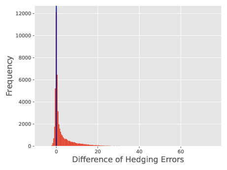
We depict the optimal hedging strategy which was computed according to Algorithm 1 with in the left panel of Figure 3.3. The relative hedging error evaluated on samples, created under uncertainty, is illustrated in the middle panel while in the right panel we provide a histogram of the difference between the absolute value of the hedging error of a hedging strategy trained on paths with fixed parameters , , , , with the absolute value of the relative hedging error of the robust strategy. The histogram shows that in most of the samples the relative hedging error of the non-robust hedge is larger than the relative hedging error of the robust hedge, an observation which is also verified through Table 3.1.


3.2.3 Hedging of path-dependent options
Next, we consider a NGA process with parameters as in (3.2) and a lookback call option with payoff function
We depict the optimal hedging strategy computed with Algorithm 1 with in the left panel of Figure 3.4 and the hedging error evaluated on samples, created according to uncertainty as in (3.2), in the middle panel of Figure 3.4. In the right panel of Figure 3.4 we compare the hedging error of a trained non-robust strategy with the hedging error of the trained robust strategy. The trained robust strategy outperforms the non-robust strategy clearly on scenarios that were created under uncertainty according to (3.2), which also can be seen in Table 3.1.
As the payoff function is path-dependent, we could improve the hedging performance further by allowing the self-financing hedging strategy to be dependent also on the running maximum. We observe that this approach indeed additionally improves the hedging performance to some degree. The results are displayed in the rightmost column of Table 3.1.


| Call | Butterfly | Lookback | |||||
|---|---|---|---|---|---|---|---|
| Parameters | fixed | robust | fixed | robust | fixed | robust | run max |
| mean | 2.0266 | 0.1924 | 0.9078 | 0.3328 | 3.5582 | 0.5857 | 0.5476 |
| std. dev. | 2.2650 | 0.1636 | 0.6548 | 0.2648 | 6.0482 | 0.7228 | 0.6305 |
3.3 Prices of hedging strategies
The presented robust hedging approach allows to respect the problem that in many situations robust price bounds such as are too expensive to have practical relevance (compare e.g. Frey and Sin 1999, Biagini and Frittelli 2004 and Neufeld 2018).
Robust price bounds may of course still be of interest, for instance to check the market for mispriced derivatives or to compute price bounds when the parameter set is chosen sufficiently small such that this approach leads to meaningful prices. To compute the price bound one may then solve the corresponding PDE (2.6) by using an explicit finite-difference method, compare also Fadina et al. 2019, where a similar approach in a nonlinear affine setting is pursued and see the companion code on https://github.com/juliansester/nga for more details.
In Figure 3.5 we provide the prices of hedging strategies for a call option with strike (as in Section 3.2.1) and of a butterfly option as in Section 3.2.2, where we consider the parameters as specified in (3.2). For comparison, we also show price bounds and computed with the mentioned explicit finite-difference method. We display prices and price bounds for different initial values of the underlying process.


The results indicate that the price of the hedging strategies, that were computed according to Algorithm 1 and which lie well between lower and upper price bound, possess great practical relevance for two reasons. First, the associated prices are neither too low nor too high to be tradable. Second and in contrast to the prices computed as maximal expectations, the prices come with a trading strategy that allows to hedge the associated financial derivative under model uncertainty.
4 Application to real-world data
In this section, we evaluate the performance of the robust deep hedging strategy on financial data. To this end, we extracted daily closing prices of of the largest constituents33 3 The considered constituents are: Apple Inc, Microsoft Corporation, Amazon.com Inc., Alphabet Inc. Class C, Berkshire Hathaway Inc. Class B, JPMorgan Chase Co., Johnson Johnson, Visa Inc. Class A, UnitedHealth Group Incorporated, NVIDIA Corporation, Procter Gamble Company, Home Depot Inc., Mastercard Incorporated Class A, Bank of America Corp, Walt Disney Company, Comcast Corporation Class A, Exxon Mobil Corporation, Adobe Inc., Verizon Communications Inc., Intel Corporation. of the US stock market index from September until April 2020 from Thomson Reuters Eikon. This time period shows a high level of uncertainty during the beginning of the COVID-19 pandemic and thus poses a challenging environment for hedging strategies.
4.1 Uncertainty in the parameter estimates
To analyze and illustrate the uncertainty present in parameter estimates, we consider parameter estimations on rolling windows. The obtained results allow us to specify the uncertainty set . These results also underline the high degree of uncertainty present in the considered data.
More precisely, we estimated the parameters under the assumption that the price observations follow generalized affine processes based on data from September 2008 until March as follows: consider the discretization of the generalized affine processes according to the Euler Maruyama scheme,
for all values of the process on observation dates (daily observations), with time difference , and normally distributed . Then, conditionally on , is normally distributed since
Accordingly, given daily prices , the log-likelihood function is given by
We consider trading days for each of the constituents of the -index. After every days we numerically maximize, by means of the Constrained Optimization by Linear Approximation (COBYLA) optimizer (Conn et al. 1997, pp. 83-108.), the log-likelihood function w.r.t. the parameters , , , , , where consists of the last trading days. The results of these estimations are illustrated for a single stock in the left panel of Figure 4.1. Moreover, in the middle panel of Figure 4.1 we display all estimates from all of the considered constituents.
The obtained estimates show a considerable variation over time. For example, the estimator of for Apple Inc. ranges from values slightly larger than to values around and highlights the advantage of using a generalized affine process rather than a simple affine process where would be fixed to . The variations of all parameter estimates over the considered 20 constituents of the S&P 500 confirm this finding. Also all other parameter estimates clearly exhibit a high degree of uncertainty.


Given this time series of historical parameter estimates, we estimate the uncertainty set by the obtained minima and maxima of the maximum-likelihood estimations. The obtained estimator is denoted by . This represents a conservative approach and takes all past observations into account. More precisely, this constitutes the smallest possible choice given the past observations. Of course, the uncertainty set could also be increased to improve robustness, which however comes at the cost of higher (and therefore potentially less attractive) derivatives’ prices and higher hedging costs.
Remark 4.1 (Historical measure vs risk-neutral measure)
In this section we are mainly interested in the hedging performance which is typically evaluated under the historical measure. However, there are also cases where one prefers the distribution under the risk-neutral measure, see for example Föllmer and Schied 2004 for a detailed exposition on various hedging concepts. In the later case one would obtain parameter estimates from liquid derivatives’ prices through calibration and then proceed analogously.
Remark 4.2 (Choice of )
We defined the parameter set by the intervals induced by the extreme maximum-likelihood-estimates. This corresponds to a conservative approach in which even outliers are deemed to be relevant for the future evolution of the underlying stochastic process. In less conservative approaches one could instead take into account inter-quartile ranges of the estimated parameters or only a grid of parameters associated to the historical estimates. The latter approach avoids that parameter combinations which did not appear in the past (e.g. large values of and usually do not occur at the same time) are considered as relevant for the future evolution.
Relying on the estimated uncertainty set we compute, according to Algorithm 1 a hedging strategy for an Asian at-the money put option with daily observations:
| (4.1) |
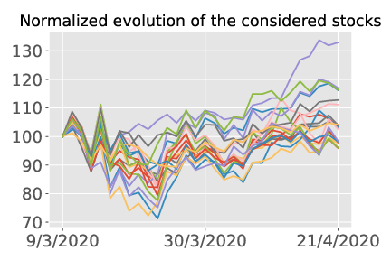
where corresponds to the respective initial spot value at March and trading days (i.e. maturity April ). Further, we compute for each constituent a hedging strategy which only takes the last maximum-likelihood estimation of the last days into account. We then evaluate, on the real price evolution of the constituents of the from March until April (compare the right panel of Figure 4.1) how both hedging strategies perform.
| Parameters | fixed | robust | fixed | fixed | fixed | fixed | fixed | Black–Scholes |
|---|---|---|---|---|---|---|---|---|
| mean | 5.8939 | 0.9014 | 0.9369 | 5.1408 | 0.9030 | 0.9433 | 2.1390 | 5.7859 |
| std. dev. | 2.7666 | 0.7705 | 0.7410 | 3.0596 | 0.7545 | 0.8073 | 1.8934 | 2.8477 |
| min. | 0.4391 | 0.0279 | 0.0104 | 0.4116 | 0.0192 | 0.0185 | 0.2303 | 2.0983 |
| max. | 12.5595 | 2.7106 | 2.6356 | 12.3456 | 2.4122 | 2.7329 | 7.4269 | 12.0025 |
For this we compare the relative hedging error of the strategies. The results are depicted in Table 4.1 and indicate that the robust hedging strategy may, in particular, perform better in periods with high volatility as in the period under consideration. In Table 4.1 we further display the hedging error of strategies that were trained, when all of the considered parameters are assumed to be contained in intervals except for a single parameter which is fixed. This analysis allows to compare and analyse the effect of robustness of single parameters on the hedging error. We observe that taking uncertainty into account is in particular important for the volatility parameters and the parameter . More precisely, while fixing the drift parameters does not lead to considerably worse hedging errors, fixing the exponent of the volatility term, and in particular the volatility parameter , significantly increases the mean and the standard deviation of the hedging error.
For comparison we also report the hedging error when applying the deep hedging approach in a (non-robust) Black--Scholes model44 4 Note that the Black–Scholes model can be considered as a special case of an NGA-process through setting for some mean and some variance ., where the parameters are estimated in a consistent manner through maximum likelihood estimation while taking into account the time series of the last trading days. The results of this hedging approach are depicted in the rightmost column of Table 4.1 and show that hedging under the Black–Scholes model leads in the considered period to a mean hedging error and standard deviation comparable to the mean hedging error of an NGA-process with fixed parameters.
This supports our choice of considering the class of generalized affine models in the robust pricing and hedging approach especially during such periods of market turmoil.
4.2 Considering a non-crisis setting
While we have now provided evidence for the outperformance of the robust hedging approach over other approaches in a crisis period, the question arises whether the approach is flexible enough to perform comparable to other approaches in periods that would be rather classified as non-crisis periods.
To this end, and to be consistent with the previously introduced methodology, we consider three additional day testing periods, starting trading days, trading days and trading days, respectively, after March . For each additional period we take new maximum-likelihood-estimations of the last days into account and evaluate, for the same payoff function (4.1), the performances of a robust hedging approach, of a non-robust hedging approach and of a hedging approach under a Black–Scholes model. The results of this study are displayed in Table 4.2 and show particularly that in these periods the mean hedging errors and the standard deviation of all approaches are reduced in comparison with the crisis period.
| Parameters | fixed | robust | Black–Scholes |
|---|---|---|---|
| mean | 0.4424 | 0.5565 | 0.4627 |
| std. dev. | 0.2272 | 0.4380 | 0.2291 |
| min. | 0.0265 | 0.0781 | 0.0170 |
| max. | 0.9608 | 2.9152 | 0.8612 |
The best performing model in these periods turns out to be the NGA-process with fixed parameters, while pursuing a robust hedging approach leads to a slightly higher hedging error and a higher standard deviation. These observations indicate that non-robust approaches perform best in regular out-of-crisis periods, whereas a robust hedging approach performs slightly worse in these periods, presumably since such hedging strategies are adjusted and calibrated to a broader range of possible future market movements. Our investigation of the performance of the hedges in the crisis period (Table 4.1) however reveals that this broad calibration can provide additional strong protection against unexpected market movements as they can be observed in crises.
4.2.1 Relation to Bayesian approaches
Instead of the presented frequentist approach, in which we use the minimal and maximal maximum-likelihood-estimations to determine the intervals representing and then to assume that the parameters of the SDE are uniformly distributed on , one might also consider other distributions: first, the empricial distribution of the parameter estimates as shown in Figure 4.1 is a natural choice. Second, a Bayesian approach for the determination of the parameter intervals can be implemented, see Duembgen and Rogers 2014 for a Bayesian approach. In this approach one starts from a prior distribution (e.g. uniform on some pre-defined intervals) for all of the parameters and then sequentially updates the resulting posterior distributions contingent on the same data which we use for the maximum-likelihood-estimations. Eventually, to determine optimal hedging strategies one modifies Algorithm 1 by drawing parameters according to the obtained posterior distributions, as already detailed in Remark 3.2. Alternatively, quasi Bayesian approaches as in Brignone et al. 2021 can be used where an asymptotic distribution of parameters is estimated from the quasi posterior distribution. Since the Bayesian approach may put relatively few weight to extreme parameters we decided to implement the presented approach which puts equal weight to all of the parameters that are considered possible. This approach is therefore robust w.r.t. extreme market movements, for what we provide evidence in the example in Section 4.
5 Conclusion
In this work we studied parameter uncertainty in the class of generalized affine processes and developed a robust hedging approach relying on deep neural networks. This approach shows resilience against unexpected changes in the dynamics of the underlying, which justifies the claimed robustness of this method. Our research is a first step towards the practical application of robust hedging approaches and still many questions remain open: the most pressing one is the practical determination of the uncertainty interval - how much risk is one willing to take by considering a smaller interval (which clearly in good weather conditions will be cheaper in pricing and hedging)? The second, highly interesting question is to incorporate transaction costs into the robust deep hedging approach, to treat other dynamics of the underlying and to consider loss functions different to the quadratic one we used in this paper.
Acknowledgements
We thank the editor and two anonymous referees for several comments which significantly improved our paper. Moreover, we are thankful to David Criens for helpful remarks. Financial support of the NAP Grant Machine Learning based Algorithms in Finance and Insurance and from Deutsche Forschungsgemeinschaft (DFG) of the grant SCHM 2160/13-1 is gratefully acknowledged.
A Appendix
A.1 Existence of generalized affine diffusions
It is well known that the state space needs to be chosen in correspondence with . In the case where , this does not pose difficulties, but in the case where some care has to be taken. The special case where is the content of Proposition 1 in Fadina et al. 2019.
We call the state space proper for the non-linear generalized affine process if for all and all . The next lemma extends Proposition 1 in Fadina et al. 2019 to the case where .
Lemma A.1
Assume that , , , and . Consider the NGA with . Then it holds for any that
Proof.
For the proof we rely on the integral test proposed in Theorem 5.2 in Criens 2020. To this end we consider a sufficiently small subset such that for all .
To begin with, we observe the estimates
| (A.1) |
with constants and .
The next step is to show that from Equation (5.5) in Criens 2020 explodes as , where
| (A.2) |
So in the following we consider . Then,
| (A.2) | (A.3) |
Then we can estimate (since ), setting ,
| (A.4) |
for some constant . Up to constants we can now estimate from below by
with Now it is easy to see that the integral on the right hand side explodes as by l’Hospital’s rule. ∎
As a consequence of Lemma A.1 we obtain that the state space is proper in the following cases:
- (i)
and ,
- (ii)
, : , , and ,
- (iii)
, : , , and .
The next proposition establishes conditions such that the set of semimartingale measures is not empty.
Proposition A.2 (Existence of generalized affine process)
Let . If assume and while for we assume and and, for , additionally . Then for all and there exists a unique strong solution to the SDE (2.1).
Proof.
The theorem follows from Corollary 5.5.16 in Karatzas and Shreve 1991 using the results from Engelbert and Schmidt (Engelbert and Schmidt 1985a, Engelbert and Schmidt 1985b). First note that in the case the function is locally integrable for any if and . If , the local integrability follows because and in that case. Further, for any we have
where Moreover, we have
i.e. the function in Corollary 5.16 in Karatzas and Shreve 1991 is given by the strictly increasing function with . Since we chose , the function satisfies the condition
Further, the conditions
- (ND)
for all and
- (LI)
for all there exists an such that
in Karatzas and Shreve 1991 are satisfied when we choose if and if . Thus, there exists a strong solution to the SDE (2.1), possibly up to an explosion time. Explosions to in finite time do not occur since we have at most linear growth.
If the state space is and , then the process does not reach zero due to Proposition 1 in Fadina et al. 2019. If , Lemma A.1 implies that again does not reach zero and the conclusion follows. ∎
A.2 Proof of the nonlinear Kolmogorov equation
In this section, we prove Theorem 2.3, which we repeat for the reader’s convenience.
Theorem 2.2
Consider a family of nonlinear generalized affine processes with state space and a Lipschitz continuous payoff function . Then,
is a viscosity solution to the PDE (2.6).
For the proof we will need some preliminary tools.
Lemma A.3
Let . For all there exists an such that for all , all and it holds that
for some constant .
The proof is a modification of the proof of Lemma 3 in Fadina et al. 2019 and Lemma 5.2 in Neufeld and Nutz 2017 and takes the generalized setting into account.
Proof.
Consider and denote by , , the semimartingale representation of from Equation (2.2). We will repeatedly use the elementary inequality
| (A.5) |
and denote .
First, the Burkholder–Davis–Gundy (BDG) inequality (see Theorem IV.4.1 in Revuz and Yor 1994) together with Jensen’s inequality and (A.5) yields for any that
| (A.6) | ||||
Note that the constant from the BDG inequality does depend on only.
We define and choose any small enough such that it satisfies
| (A.7) |
Let us verify that such a fixed satisfies the desired property: by the very definition of , we have on that both and are bounded from above by and , respectively, since they are GA-dominated. This, together with Jensen’s inequality, yields that
| (A.8) | ||||
Since and , we have that
Then,
| (A.8) | |||
Since the drift is affine dominated, we obtain in a similar way that
Inserting these inequalities into (A.6), considering , and noting that implies that
| (A.9) | |||||
Since and we chose such that (A.7) holds, we obtain for the constant , being independent of , that
As was chosen arbitrarily, the claim is proven. ∎
Lemma A.4
Consider a nonlinear generalized affine process and a derivative with Lipschitz-continuous payoff function . Then the value function
is jointly continuous. In particular, is locally -Hölder continuous in and Lipschitz-continuous in .
Proof.
The statement follows similarly to Lemma 4 in Fadina et al. 2019 and Lemma 5.3 in Neufeld and Nutz 2017. For and fixed it holds that
where is the Lipschitz constant of the function . Thus, the value function is Lipschitz-continuous in .
Proof.
(of Theorem 2.3) The proof essentially follows the well-known standard arguments in stochastic control, see e.g., the proof of (Neufeld and Nutz 2017, Proposition 5.4).
By Lemma A.4, is continuous on , and we have by the definition of . We show that is a viscosity subsolution of the nonlinear affine PDE defined in (2.7); the supersolution property is proved similarly. We remark that in the subsequent lines within this proof, is a constant whose values may change from line to line.
Let and let be such that and . By the dynamic programming principle obtained in Proposition 2.2, we have for any that
| (A.10) |
Fix any , denote as above by the differential characteristics of the continuous semimartingale under , and denote by the -local martingale part of the -semimartingale . Then, Itô’s formula yields
| (A.11) |
As , is uniformly bounded,we see that for small enough the local martingale part in (A.11) is in fact a true martingale, starting at . In particular, its expectation vanishes. The next step is to estimate the expectation of the other terms. In this regard, note that
| (A.12) |
Since , is Lipschitz. Hence, we obtain with the constant together with Lemma A.3 that for small enough ,
| (A.13) |
Inserting (A.13) into (A.12) yields
| (A.14) | |||||
The same argument applied to leads to
| (A.15) |
and we obtain that
| (A.16) | |||||
Moreover, by a similar calculation, we have
| (A.17) |
As above, we write for an element in . Then, by taking expectations in (A.11) and using (A.12)–(A.17) yields
| (A.18) | |||||
Here, the supremum turns out to be . Note that by the very definition of ,
Therefore, by using that , the definition of the constant and Lemma A.3, we have
| (A.19) | |||||
Combining (A.18)–(A.19) yields
| (A.20) |
for some constant which is independent of . As the choice of was arbitrary, we deduce from (A.2) that
| (A.21) |
By dividing first in (A.21) by and then letting go to zero, we obtain that
which proves that is indeed a viscosity subsolution as desired. ∎
References
- (1)
- Abadi et al. (2016) Abadi, M., Barham, P., Chen, J., Chen, Z., Davis, A., Dean, J., Devin, M., Ghemawat, S., Irving, G., Isard, M. et al. (2016), Tensorflow: A system for large-scale machine learning, in ‘12th USENIX symposium on operating systems design and implementation (OSDI 16)’, pp. 265–283.
- Acciaio et al. (2016) Acciaio, B., Beiglböck, M., Penkner, F. and Schachermayer, W. (2016), ‘A model-free version of the fundamental theorem of asset pricing and the super-replication theorem’, Mathematical Finance 26(2), 233–251.
- Aksamit et al. (2020) Aksamit, A., Hou, Z. and Obłój, J. (2020), ‘Robust framework for quantifying the value of information in pricing and hedging’, SIAM Journal on Financial Mathematics 11(1), 27–59.
- Akthari et al. (2020) Akthari, B., Biagini, F., Mazzon, A. and Oberpriller, K. (2020), ‘Generalized Feynman-Kac formula under volatility uncertainty’, arXiv preprint arXiv:2012.08163 .
- Avellaneda et al. (1995) Avellaneda, M., Levy, A. and Parás, A. (1995), ‘Pricing and hedging derivative securities in markets with uncertain volatilities’, Appl. Math. Finance 2(2), 73–88.
- Barnett et al. (2020) Barnett, M., Brock, W. and Hansen, L. P. (2020), ‘Pricing uncertainty induced by climate change’, The Review of Financial Studies 33(3), 1024–1066.
- Beiglböck et al. (2013) Beiglböck, M., Henry-Labordère, P. and Penkner, F. (2013), ‘Model-independent bounds for option prices—a mass transport approach’, Finance and Stochastics 17(3), 477–501.
- Biagini and Frittelli (2004) Biagini, S. and Frittelli, M. (2004), ‘On the super replication price of unbounded claims’, The Annals of Applied Probability 14(4), 1970–1991.
- Bouchard et al. (2015) Bouchard, B., Nutz, M. et al. (2015), ‘Arbitrage and duality in nondominated discrete-time models’, Annals of Applied Probability 25(2), 823–859.
- Brignone et al. (2021) Brignone, R., Gonzato, L. and Lütkebohmert, E. (2021), ‘Efficient quasi-Bayesian estimation of affine option pricing models using risk-neutral cumulants’. Working paper.
- Buehler et al. (2019) Buehler, H., Gonon, L., Teichmann, J. and Wood, B. (2019), ‘Deep hedging’, Quantitative Finance 19(8), 1271–1291.
- Cao et al. (2021) Cao, J., Chen, J., Hull, J. and Poulos, Z. (2021), ‘Deep hedging of derivatives using reinforcement learning’, The Journal of Financial Data Science 3(1), 10–27.
- Carbonneau (2021) Carbonneau, A. (2021), ‘Deep hedging of long-term financial derivatives’, Insurance: Mathematics and Economics 99, 327–340.
- Carbonneau and Godin (2021) Carbonneau, A. and Godin, F. (2021), ‘Equal risk pricing of derivatives with deep hedging’, Quantitative Finance 21(4), 593–608.
- Chen and Wan (2021) Chen, Y. and Wan, J. W. (2021), ‘Deep neural network framework based on backward stochastic differential equations for pricing and hedging American options in high dimensions’, Quantitative Finance 21(1), 45–67.
- Cheridito et al. (2017) Cheridito, P., Kupper, M. and Tangpi, L. (2017), ‘Duality formulas for robust pricing and hedging in discrete time’, SIAM Journal on Financial Mathematics 8(1), 738–765.
- Cohen and Tegnér (2017) Cohen, S. N. and Tegnér, M. (2017), European option pricing with stochastic volatility models under parameter uncertainty, in ‘International symposium on BSDEs’, Springer, pp. 123–167.
- Conn et al. (1997) Conn, A. R., Scheinberg, K. and Toint, P. L. (1997), ‘On the convergence of derivative-free methods for unconstrained optimization’, Approximation theory and optimization: tributes to MJD Powell pp. 83–108.
- Cox and Obłój (2011) Cox, A. M. and Obłój, J. (2011), ‘Robust pricing and hedging of double no-touch options’, Finance and Stochastics 15(3), 573–605.
- Criens (2020) Criens, D. (2020), ‘No arbitrage in continuous financial markets’, Mathematics and Financial Economics 14(3), 461–506.
- Cuchiero et al. (2020) Cuchiero, C., Khosrawi, W. and Teichmann, J. (2020), ‘A generative adversarial network approach to calibration of local stochastic volatility models’, Risks 8(4), 101.
- Denk (2021) Denk, L. (2021), Pricing und Hedging von Derivaten unter Parameterunsicherheit, Master’s thesis, University of Freiburg.
- Dolinsky and Soner (2014) Dolinsky, Y. and Soner, H. M. (2014), ‘Martingale optimal transport and robust hedging in continuous time’, Probability Theory and Related Fields 160(1-2), 391–427.
- Duembgen and Rogers (2014) Duembgen, M. and Rogers, L. (2014), ‘Estimate nothing’, Quantitative Finance 14(12), 2065–2072.
- Eckstein et al. (2021) Eckstein, S., Guo, G., Lim, T. and Obłój, J. (2021), ‘Robust pricing and hedging of options on multiple assets and its numerics’, SIAM Journal on Financial Mathematics 12(1), 158–188.
- El Karoui and Tan (2013) El Karoui, N. and Tan, X. (2013), ‘Capacities, measurable selection and dynamic programming part II: Application in stochastic control problems’, arXiv:1310.3364v2 .
- Engelbert and Schmidt (1985a) Engelbert, H. J. and Schmidt, W. (1985a), On one-dimensional stochastic differential equations with generalized drift, in ‘Stochastic Differential Systems Filtering and Control’, Springer, pp. 143–155.
- Engelbert and Schmidt (1985b) Engelbert, H.-J. and Schmidt, W. (1985b), ‘On solutions of one-dimensional stochastic differential equations without drift’, Zeitschrift für Wahrscheinlichkeitstheorie und verwandte Gebiete 68(3), 287–314.
- Fadina et al. (2019) Fadina, T., Neufeld, A. and Schmidt, T. (2019), ‘Affine processes under parameter uncertainty’, Probability, Uncertainty and Quantitative Risk 4(5).
- Föllmer and Schied (2004) Föllmer, H. and Schied, A. (2004), Stochastic Finance, Walter de Gruyter, Berlin.
- Fouque and Ren (2014) Fouque, J.-P. and Ren, B. (2014), ‘Approximation for option prices under uncertain volatility’, SIAM Journal on Financial Mathematics 5(1), 360–383.
- Frey and Sin (1999) Frey, R. and Sin, C. A. (1999), ‘Bounds on european option prices under stochastic volatility’, Mathematical Finance 9(2), 97–116.
- Geuchen and Schmidt (2021) Geuchen, B. and Schmidt, T. (2021), ‘Non-linear affine processes and path-dependent derivatives’, in preparation .
- Gierjatowicz et al. (2020) Gierjatowicz, P., Sabate-Vidales, M., Siska, D., Szpruch, L. and Zuric, Z. (2020), ‘Robust pricing and hedging via neural sdes’, Available at SSRN 3646241 .
- Gümbel and Schmidt (2020) Gümbel, S. and Schmidt, T. (2020), ‘Machine learning for multiple yield curve markets: fast calibration in the Gaussian affine framework’, Risks 8(2), 50.
- Hobson (1998) Hobson, D. G. (1998), ‘Robust hedging of the lookback option’, Finance and Stochastics 2(4), 329–347.
- Horváth et al. (2021) Horváth, B., Teichmann, J. and Zuric, Z. (2021), ‘Deep hedging under rough volatility’, Available at SSRN 3778043 .
- Hou and Obłój (2018) Hou, Z. and Obłój, J. (2018), ‘Robust pricing–hedging dualities in continuous time’, Finance and Stochastics 22(3), 511–567.
- Karatzas and Shreve (1991) Karatzas, I. and Shreve, S. (1991), Brownian Motion and Stochastic Calculus, 2nd edn, Springer.
- Kingma and Ba (2014) Kingma, D. P. and Ba, J. (2014), ‘Adam: A method for stochastic optimization’, arXiv preprint arXiv:1412.6980 .
- Lütkebohmert and Sester (2019) Lütkebohmert, E. and Sester, J. (2019), ‘Tightening robust price bounds for exotic derivatives’, Quantitative Finance 19(11), 1797–1815.
- Nadtochiy and Obłój (2017) Nadtochiy, S. and Obłój, J. (2017), ‘Robust trading of implied skew’, International Journal of Theoretical and Applied Finance 20(02), 1750008.
- Neufeld (2018) Neufeld, A. (2018), ‘Buy-and-hold property for fully incomplete markets when super-replicating markovian claims’, International Journal of Theoretical and Applied Finance 21(08), 1850051.
- Neufeld and Nutz (2017) Neufeld, A. and Nutz, M. (2017), ‘Nonlinear Lévy processes and their characteristics’, Trans. Am. Math. Soc. 369(1), 69–95.
- Neufeld and Sester (2021a) Neufeld, A. and Sester, J. (2021a), ‘A deep learning approach to data-driven model-free pricing and to martingale optimal transport’, arXiv preprint arXiv:2103.11435 .
- Neufeld and Sester (2021b) Neufeld, A. and Sester, J. (2021b), ‘Model-free price bounds under dynamic option trading’, SIAM Journal on Financial Mathematics 12(4), 1307–1339.
- Petersen (2020) Petersen, P. C. (2020), ‘Neural network theory’, University of Vienna .
- Revuz and Yor (1994) Revuz, D. and Yor, M. (1994), Continuous Martingales and Brownian Motion, Springer.
- Ruf and Wang (2020) Ruf, J. and Wang, W. (2020), ‘Neural networks for option pricing and hedging: a literature review’, Journal of Computational Finance, Forthcoming .
- Wilmott and Oztukel (1998) Wilmott, P. and Oztukel, A. (1998), ‘Uncertain parameters, an empirical stochastic volatility model and confidence limits’, International Journal of Theoretical and Applied Finance 1(1), 175–189.