Edge states of a diffusion equation in one dimension:
Rapid heat conduction to the heat bath
Abstract
We propose a one-dimensional (1D) diffusion equation (heat equation) for systems in which the diffusion constant (thermal diffusivity) varies alternately with a spatial period . We solve the time evolution of the field (temperature) profile from a given initial distribution, by diagonalising the Hamiltonian, i.e., the Laplacian with alternating diffusion constants, and expanding the temperature profile by its eigenstates. We show that there are basically phases with or without edge states. The edge states affect the heat conduction around heat baths. In particular, rapid heat transfer to heat baths would be observed in a short time regime, which is estimated to be s for m system and s for m system composed of two kinds of familiar metals such as titanium, zirconium and aluminium, gold, etc. We also discuss the effective lattice model which simplifies the calculation of edge states up to high energy. It is suggested that these high energy edge states also contribute to very rapid heat conduction in a very short time regime.
I Introduction
The bulk-edge correspondence Hatsugai 1993a; Hatsugai 1993b is recognized as one of fundamental concepts in physics Hasan and Kane 2010; Qi and Zhang 2011. The original idea was proposed to answer the question of whether the quantum Hall effect (QHE) is a bulk or edge-state property Hatsugai 1993a; Hatsugai 1993b, but it has now become a way to more broadly characterize topological insulators. Indeed, it has been playing a central role in the development of topological insulators and superconductors Kane and Mele 2005; Qi et al. 2008. Remarkably, it has been extended to classical systems such as photonic crystals Raghu and Haldane 2008; Haldane and Raghu 2008; Wang et al. 2009; Ozawa et al. 2019; Kivshar 2019, phononic systems Prodan and Prodan 2009; Savin et al. 2010; Kane and Lubensky 2013; Kariyado and Hatsugai 2015; Süsstrunk and Huber 2015; Chien et al. 2018; Yoshida and Hatsugai 2019; Kivshar 2019, electrical circuits Albert et al. 2015; Lee et al. 2018; Helbig et al. 2020; Yoshida et al. 2020, hydrodynamics Delplace et al. 2017; Sone and Ashida 2019, and so on.
Recently, the importance of edge states was also pointed out in diffusion phenomena Yoshida and Hatsugai 2021. This implies that edge states would have a large effect not only on propagating wave systems but also diffusive systems such as heat conduction. In particular, in Ref. Yoshida and Hatsugai 2021, a lattice model was introduced by coarsely discretizing the diffusion equation, and their prediction was indeed observed experimentally Hu et al. 2021; Qi et al. 2021. Here, our question is whether the heat conduction in a continuous medium that is not necessarily protected by symmetry is affected by edge states or not. This attempt is also aimed at understanding the role of edge states in more mundane phenomena that are not necessarily of direct relationship with topology.
In this paper, we examine the one-dimensional (1D) diffusion equation with position-dependent diffusion constant, especially paying attention to the role of edge states. In general, one dimensional systems would show anomalous heat conduction due to anomalous diffusion Li and Wang 2003. However, we assume systems governed by the normal diffusion as well as the normal Fourier or Fick law, and hence, consider the conventional diffusion equation. Nevertheless, the diffusion equation shows a characteristic behavior when systems allow edge states.
To examine the effect of edge states, we propose 1D diffusion equation with periodic array of two distinct diffusion constants. Most coarse discretization of such an equation with respect to space leads to the Su-Schriffer-Heeger (SSH) Hamiltonian Su et al. 1979, which was already studied in Yoshida and Hatsugai 2021. In this case, the relationship between edge states and bulk topology is manifest. In this paper, we investigate the opposite limit, a continuous equation for a continuous medium directly, in which the bulk-edge correspondence is rather vague. Namely, a continuous medium allows various boundary conditions, and the bulk topological invariant protected by inversion symmetry does not necessarily guarantee the edge states on boundaries which do not respect inversion symmetry. Nevertheless, even without inversion symmetry, we find that there appear many edge states, and the diffusion of initial heat distributions given near a boundary is accelerated by edge states in a short time regime. These edge states are surely related to those that appear for a boundary condition respecting inversion symmetry. Thus, we claim that even if boundary conditions breaks symmetry, some of them disappear but others remain persistently.
This paper is organized as follows. In Sec. II, we derive a diffusion equation with an -dependent diffusion constant. We regard it as an imaginary-time Schrödinger equation and solve its initial value problem by using the complete set of eigenstates. To this end, we solve the eigenvalue equation of the Hamiltonian first by the Bloch techniques for the bulk system, and next by the Fourier series expansion under Dirichlet boundary condition for a finite system in contact with the heat baths. In the latter system, we find the appearance of edge states localized at the boundary, which are not present in the bulk system. Solving the initial value problem, we find rapid heat transfer to the heat bath at the boundary, which can be understood as the consequence of edge states. In Sec. III, we next discretize the diffusion equation and derive an effective lattice model. This enables us to obtain the edge states very simply up to very high energies. In Sec. IV, we give summary and discussion including the experimental feasibility.
II Diffusion equation in one-dimension
We consider generic systems described by a one-dimensional diffusion equation whose diffusion constant takes two values periodically in space. We assume purely one-dimensional arrays of different materials, or some layered systems stacked in one direction but uniform in the directions perpendicular to it.
For a while, we assume a diffusion equation with a position-dependent diffusion constant generically. Let be the local field at time . We assume the Fick law
| (1) |
where stands for the current density. Then, the continuity equation reads
| (2) |
These equations lead to the following diffusion equation,
| (3) |
In the following, we regard Eq. (3) as an imaginary-time Schrödinger equation and consider the eigenstates of the Hamiltonian operator
| (4) |
Note that the Hamiltonian in Eq. (4) is Hermitian.
In what follows, we are mainly interested in the heat conduction. Then, to be precise, it is necessary to take into account the -dependence of two constants characterizing the materials, i.e., the heat capacity and thermal conductivity. As a result, the Fourier law with a -dependent thermal conductivity and the continuity equation with a -dependent heat capacity lead to more complicated equation than Eq. (4). In particular, the Hamiltonian becomes non-Hermitian in general. However, for the sake of simplicity in this paper, we consider only thermal diffusivity as a -dependent parameter, ignoring the derivative of the heat capacity. Even with this simpler equation, it is possible to analyze edge states, since they have topological origin, albeit indirectly, as we will see. This guarantees the robustness of edge states even if we have resort to any approximations, as long as they are small.
More basically, if one derives the diffusion equation in inhomogeneous systems microscopically, one starts with the Langevin equation, and derives the Fokker-Planck equation. Here, it should be noted that the Langevin equation allows several interpretations related to the examined process and the nature of the noise, leading to different diffusion equations Leibovich and Barkai 2019; dos Santos et al. 2020. Among them, Itô and Stratonovich types yield non-hermitian Hamiltonians generically, whereas in this paper, we adopt the Hänggi-Klimontovich type Hanggi 1982; Klimontovich 1990 which allows hermitian Hamiltonian (4) for simplicity. We also mention that the Hamiltonian (4) can be interpreted as a quantum mechanical kinetic Hamiltonian with a position-dependent mass da Costa et al. 2020.
II.1 Bulk spectrum
We now assume . Then, the Bloch theorem states that the eigenfunction can be written as
| (5) |
where and the Bloch state is periodic, . For , the eigenvalue equation (4) becomes
| (6) |
Now, let us expand the periodic functions and in the Fourier series,
| (7) |
with . Substituting these into Eq. (6), we have
| (8) |
where the -dependence of has been suppressed, and the Hamiltonian is given by
| (9) |
Thus, the Fourier coefficient determines the diffusion phenomena in the present system.
 |
To be concrete, let us assume
as illustrated in Fig. 1. This can be expressed in the Fourier series such that
| (12) |
where and .
In this paper, we assume one typical diffusion constant , and consider systems composed of materials with and . The effect of the ratio will be discussed in Sec. IV. In Fig. 2, we show some spectra of the Hamiltonian (9). The Hamiltonian of the uniform system with () is a simple Laplacian with the dispersion,
| (13) |
as seen in Fig. 2 (a). Once is introduced, spectrum has a gap at multiples of . As a result, the lowest band of system approaches the band of the uniform system with smaller diffusion constant , not that of uniform systems with .
 |
So far we have discussed the gapped spectrum of the system with . It may be needless to say that the spectrum for the opposite series of the diffusion constant, , is completely the same. Switch between and is achieved by the transformations
- (r)
reflection:
- (t)
translation: .
These symmetries are for the bulk systems, but approximately apply to the finite systems, as seen in Sec. II.2.
II.2 Finite system with boundaries
Let us consider the system with length and impose the Dirichlet boundary condition which implies, in the case of heat conduction, a system sandwiched by heat baths at both ends. See Fig. 3. We assume that the field describes the difference of the temperatures , where and stand for the temperatures of the material and of the heat baths, respectively. Therefore, we set for . We also assume that within the temperature range of interest, the heat conduction in each layer follows the usual diffusion equation with thermal diffusivity or .
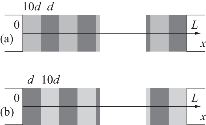 |
Then, we can expand in the following Fourier series
| (14) |
where is real, and . Substituting Eq. (14) as well as Eq. (7) into Eq. (4), we have the Hamiltonian
| (15) |
Derivations and the definitions of matrix elements are given in Appendix A. In numerical calculations below, we introduce a cutoff for the Hamiltonian (15).
 | |
 |
 |
In Fig. 4 (a), we show the spectra of the systems with length , solving the eigenvalue equation . Here, we emphasize that the system with gives exactly the same spectrum, including the edge states, as the system with : The differences lies in the wave functions. To see this, we show in Fig. 4 (b), the eigenfunctions (), corresponding to the lowest edge states. The red and blue curves are for the systems with and , respectively, corresponding to Fig. 3(a) and 3(b). In the cases and , the edge states appear on the left and right ends, respectively. For reference sake, we also show one example of eigenfunction of the extended state in Fig. 4 (c). The eigenfunctions of the edge states and extended states have a clear distinction: While the extended states are related with each other by reflection (r) as well as translation (t), the edge states are related only by reflection (t).
II.3 Time evolution
Let be the normalized -th eigenstate of the Hamiltonian in Eq. (15). Since the Hamiltonian is Hermitian, the eigenfunctions form a complete orthonormal basis,
| (16) |
from which it follows
| (17) |
Let be a given initial distribution of . Then, the time evolution of is induced by the Hamiltonian such that
| (18) |
where stands for the inner product of two real functions.
 |
 |
In what follows, we give some numerical results for the initial state
where , implying that a sequence of several unit cells has in the background of .
II.3.1 Role of edge states
We first see that conventional bulk diffusion properties are indeed governed by a smaller diffusion constant rather the larger one . To this end, let us give an initial nonzero field at the center of the system, . Then, edge states should have nothing to do with the diffusion as far as . As shown in Fig. 5 (a), starting from such an initial state, the profile of at finite is, regardless of or , similar to the uniform system with smaller diffusion constant denoted by the black solid curve. The red and blue curves are slightly shifted to the opposite directions. Physically, it is quite natural, while mathematically, it is induced by (t) symmetry of the extended eigenfunctions shown in Fig. 4 (c).
In contrast, if one gives a finite field at the boundary unit cell in contact with the heat bath, the diffusion of depends strongly on or . The red curve in Fig. 5 (b) shows more rapid diffusion than the blue curve. On one hand, such a difference seems quite natural, since the initial nonzero field flows directly to the heat bath through the diffusion constant next to the bath. Indeed, in , the red (blue) curve is just on the dashed (solid) curve which is the profile with the larger (smaller) diffusion constant. On the other hand, from the point of view of the formula (18), the difference between the red and blue curves is attributed to the edge states, since in the two systems, (i) the spectra are exactly the same and (ii) bulk states are related with each other by the translation (t), whereas only the edge states break the translation (t).
 |
 |
To clarify this more quantitatively, let us define “internal energy” by
| (21) |
In Fig. 6, we show and for the system in Fig. 5 (b). Figure 6 (a) manifestly shows that the heat transfer to the heat bath is governed by the leftmost diffusion constants. To see the effects of the edge states, we calculate the diffusion from the unit cell at the left edge, shown in Fig. 6 (b). In the case of , there are no low-energy edge states, implying that the diffusion occurs through the bulk extended states only. Contrary to this, in the case of , quite rapid diffusion is induced at very short time . This is mainly due to high-energy edge states, as will be discussed in Sec. III. Around , the lowest energy edge state with the energy dominates the main diffusion which is suggested by the coincidence with the green dashed line.
II.3.2 Rapid heat conduction
Since the localization length of the lowest edge state shown in Fig. 4 (b) is about unit cells (See also Sec. III), the effect of the edge state would be more pronounced if we start from a wider distribution of the initial temperature near the boundary.
 |
 |
In Fig. 7, the temperature profile starting from the initial distribution is shown. Remarkably, rapid heat transfer from the left end to the heat bath is observed for the system. Indeed, comparing the red curve with the dotted curve, we see that the temperature at each point of the left end cell with is about half of a uniform system with . Since the temperature profile at is determined by the balance between the heat escaping into the left heat bath and the heat coming in from the right , the temperature profile of the uniform system with the dashed line which is higher than the red curves is due to larger heat transfer from the right than that of the alternating system. This fact, that heat far from the boundary influences the boundary temperature profile, suggests that the temperature profile is determined by the extended states in the uniform system. On the other hand, the temperature profile in of the alternating system denoted by the red curve is not affected by the heat far from the boundary and is quite similar to that in Fig. 5 (b), as a result. This suggests that such temperature profile is dominated by the edge states.
III Effective lattice model
So far we have discussed that the edge states modify the short-time heat conduction near the boundaries in contact with heat baths. Eigenvalues and eigenstates under the Dirichlet boundary condition have been obtained using the Fourier series expansion. In this approach, one cannot judge an eigenstate to be a bulk state or an edge state unless one has a look at the profile of the eigenfunction. On the other hand, for tight-binding models, it is very simple to obtain only the edge states separated from the bulk states Dwivedi and Chua 2016; Duncan et al. 2018; Kunst et al. 2017; Kunst et al. 2018; Kunst et al. 2019a; Kunst et al. 2019b; Pletyukhov et al. 2020; Fukui 2020. In this section, in order to discuss the edge states of the diffusion equation more simply, we derive an effective tight-binding Hamiltonian by discretizing the continuum Hamiltonian in Eq. (4).
 |
To this end, let us define the lattice labeled by (), where is a lattice constant, and introduce
| (22) |
where . On the lattice, we replace the differential operator in Eq. (4) into difference operators defined by and . The Hamiltonian in Eq. (4) can be discretized such that
| (23) |
It may be convenient to regard sites as a unit cell, as illustrated in Fig. 8. Namely, we label the sites such that
| (24) |
Then, the Hamiltonian becomes matrix operator labelled by .
Since the unit cell can be chosen by an arbitrary sequential sites, let us define more generic Hamiltonian such that
where and stand for the forward and backward shift operators defined by and . The bulk spectrum can be determined by setting and . The wavenumber of this lattice model, expressed in terms of the wavenumber of the Bloch state in Eq. (5), implies . Here, we choose , and for the effective lattice Hamiltonian in Sec. II.
III.1 Edge states
For tight-binding models, the transfer matrix method is the standard technique to derive the edge states embedded in the bulk Hatsugai 1993a; Hatsugai 1993b. Alternatively, the edge states located at the left end and at the right end can be separately computed based on the Hermiticity of the Hamiltonian, as proposed in Ref. Fukui 2020. In this paper, we use the latter method to compute the edge states, which may be useful for Hamiltonians with large dimensions such as the discretized Hamiltonian of the present system. This method is briefly summarized in Appendix B.
III.1.1 Edge state Hamiltonian
As discussed in Appendix B, the edge states localized at the left end are described by the Hamiltonian obtained by neglecting the th row and column of the Hamiltonian (III),
The eigenstates of this Hamiltonian are not necessarily true edge states of the Hamiltonian (III): We can choose the edge states by requiring that the localization length should be positive,
| (38) |
The edge states at the right end can be also derived in a similar way Fukui 2020.
 |
In Fig. 9, we plot the eigenvalues of the left and right edge state Hamiltonians by colored dots on the background of the bulk bands computed by the Hamiltonian (III). As in the case of the continuum model in Sec. II, the lattice model with shows the edge states only at the left end. Table 1 shows the localization length of the edge states. The lowest edge state has unit cell localization length, implying that the boundary heat conduction is not affected by the initial heat in , as indeed observed in Sec. II.3.2.
 |
In addition to the edge states in Fig. 9, there can be many other edge states up to very high energies. We extend Fig. 9 up to very high energies in Fig. 10. The system with is indeed the case, whereas the system with never show edge states in all energy regime. Such difference affects the heat conduction at very short time discussed in Sec. II.3.1.
| State # | 1 | 2 | 3 | 4 | 5 | 6 |
|---|---|---|---|---|---|---|
| 3.02 | 8.59 | 17.83 | 59.10 | 77.59 | 103.89 | |
| 2.20 | 0.88 | 3.23 | 1.89 | 0.98 | 7.36 |
III.1.2 Topological properties
In this section, we argue that the edge states obtained so far have intimate relationship with the topological property of the bulk system. For the continuum model, we have chosen the area surrounded by the dotted line in Fig.1 as the unit cell. Correspondingly, we have chosen the unit cell of the lattice model to match the continuum model. In this case, the model has broken inversion symmetry. However, the unit cell in Fig. 1 and corresponding lattice model has inversion symmetry. Then, the Berry phase of each band is quantized as or , which serves as the topological invariant Ryu and Hatsugai 2002. It should be noted that bulk spectrum does not depend on the choice of a specific unit cell. The choice of a unit cell means the choice of the boundaries.
 |
 |
In Fig. 11, we show the spectra of the lattice model with inversion symmetry. Each bulk band is distinguished as a solid curve (Berry phase ) or a dashed curve (Berry phase ). With inversion symmetry, the left end and the right end are completely the same, so that the same edge states appear on both ends. In this system, we can check the bulk-edge correspondence, namely, an edge state appears if the sum of Berry phases of the lower bulk bands are modulo . Comparing Figs. 9, 10, and 11, we conclude that although the edge states in Figs. 9 and 10 are not directly protected by inversion symmetry, their origin lies in the symmetry-protected edge states: Symmetry breaking boundaries make some of them disappear, whereas others remain.
IV Summary and discussion
We have examined the 1D diffusion equation with the SSH-like alternating diffusion constants. Since the diffusion equation can be regarded as an imaginary-time Schödinger equation, we have calculated the eigenvalues and eigenstates of the Hamiltonian which is the spatial part of the diffusion equation. We have shown that the SSH-like structure yields spectral gaps, and if boundaries are introduced, there appear edge states within the bulk gaps. These edge states have a significant effect on the diffusion process in a short-time regime near boundaries: Rapid heat conduction to the heat bath is expected if a boundary allows edge states.
 |
Finally, let us discuss the experimental feasibility. The model includes basically two parameters, and . We assume , for simplicity. In this case, the model has edge states at the left end, which are characterized well by rearranged two parameters and . The key parameter is rather than their ratio . To see this, we show the bulk and edge states energies in Fig. 12, changing the value of such that (and in the inset in Fig. 9). The energies and the localization lengths vary, but qualitative difference is rather small.
Next, let us consider the material-dependence of the parameter . The titanium and zirconium are candidates of materials with smaller thermal diffusivities, m2/s, and hence, fixing the length of the unit cell as m, we have s. Combined with materials having larger thermal diffusivities such as carbon (), iron (), lead (), aluminum (), and gold (), rapid heat transfer through edge states discussed in Sec. II.3.2 would be observed up to s for samples with m, and s for samples with m.
Acknowledgements.
This work was supported in part by Grants-in-Aid for Scientific Research Numbers 17K05563, 17H06138, JP21K13850, and JP20H04627 from the Japan Society for the Promotion of Science.Appendix A Fourier series expansion under the Dirichlet boundary condition
According to the Dirichlet boundary condition (14), It may be convenient to rewrite Eq. (12) with respect to ,
| (39) |
Substituting Eq. (39) as well as (14) into Eq. (4), and using
| (40) |
where , we obtain the Hamiltonian (15). The matrix elements associated with the couplings with are defined by
| (41) |
with .
Appendix B Edge state Hamiltonian
The eigenvalue equation of the Hamiltonian (23) can be written as
| (42) |
where and are matrices proportional to and , and is the remaining part of the Hamiltonian in Eq. (III). As noted in Sec. II, the continuum Hamiltonian is Hermitian. As a result, the discretized Hamiltonian (III) is also Hermitian as far as the system is defined on the infinite line. However, if the system has a boundary, the Hamiltonian is not necessarily Hermitian because of the boundary term due to the summation by parts. As proposed in Ref. Fukui 2020, imposing the Hermiticity condition naturally leads to a theoretical framework that allows us to discuss only the edge states in isolation from the bulk states.
Assume that the system has a boundary at and is defined on the semi-infinite line . Then, Hermiticity is guaranteed by introducing the reference state and requiring
| (43) |
It is readily find that the state satisfies Eq. (43), where is a vector with components. Taking as a reference state, we can obtain the edge states at the left end by assuming the Bloch-like sates with . Note that and are the momentum and the localization length of the edge state, respectively. The eigenvalue equation then becomes
Therefore, the edge states are eigenstates of the upper dimensional matrix in Eq. (III.1.1) with the constraint,
| (65) |
which follows from the condition to be satisfied by the lowest component in Eq. (B). This equation gives the localization length and the momentum of the edge states by the wave functions.
References
- Hatsugai (1993a) Y. Hatsugai, Physical Review Letters 71, 3697 (1993a), URL http://link.aps.org/doi/10.1103/PhysRevLett.71.3697.
- Hatsugai (1993b) Y. Hatsugai, Physical Review B 48, 11851 (1993b), URL https://link.aps.org/doi/10.1103/PhysRevB.48.11851.
- Hasan and Kane (2010) M. Z. Hasan and C. L. Kane, Reviews of Modern Physics 82, 3045 (2010).
- Qi and Zhang (2011) X.-L. Qi and S.-C. Zhang, Reviews of Modern Physics 83, 1057 (2011).
- Kane and Mele (2005) C. L. Kane and E. J. Mele, Physical Review Letters 95, 146802 (2005).
- Qi et al. (2008) X.-L. Qi, T. L. Hughes, and S.-C. Zhang, Physical Review B 78, 195424 (2008).
- Raghu and Haldane (2008) S. Raghu and F. D. M. Haldane, Physical Review A 78, 033834 (2008), URL https://link.aps.org/doi/10.1103/PhysRevA.78.033834.
- Haldane and Raghu (2008) F. D. M. Haldane and S. Raghu, Physical Review Letters 100, 013904 (2008), URL https://link.aps.org/doi/10.1103/PhysRevLett.100.013904.
- Wang et al. (2009) Z. Wang, Y. Chong, J. D. Joannopoulos, and M. Soljačić, Nature 461, 772 EP (2009), URL https://doi.org/10.1038/nature08293.
- Ozawa et al. (2019) T. Ozawa, H. M. Price, A. Amo, N. Goldman, M. Hafezi, L. Lu, M. C. Rechtsman, D. Schuster, J. Simon, O. Zilberberg, et al., Reviews of Modern Physics 91, 015006 (2019), URL https://link.aps.org/doi/10.1103/RevModPhys.91.015006.
- Kivshar (2019) Y. Kivshar, Low Temperature Physics 45, 1026 (2019), URL https://doi.org/10.1063/1.5121273.
- Prodan and Prodan (2009) E. Prodan and C. Prodan, Physical Review Letters 103, 248101 (2009), URL https://link.aps.org/doi/10.1103/PhysRevLett.103.248101.
- Savin et al. (2010) A. V. Savin, Y. S. Kivshar, and B. Hu, Physical Review B 82, 195422 (2010), URL https://link.aps.org/doi/10.1103/PhysRevB.82.195422.
- Kane and Lubensky (2013) C. L. Kane and T. C. Lubensky, Nature Physics 10, 39 EP (2013), URL https://doi.org/10.1038/nphys2835.
- Kariyado and Hatsugai (2015) T. Kariyado and Y. Hatsugai, Scientific Reports 5, 18107 EP (2015), URL https://doi.org/10.1038/srep18107.
- Süsstrunk and Huber (2015) R. Süsstrunk and S. D. Huber, Science 349, 47 (2015), URL https://science.sciencemag.org/content/sci/349/6243/47.full.pdf.
- Chien et al. (2018) C.-C. Chien, K. A. Velizhanin, Y. Dubi, B. R. Ilic, and M. Zwolak, Physical Review B 97, 125425 (2018), URL https://link.aps.org/doi/10.1103/PhysRevB.97.125425.
- Yoshida and Hatsugai (2019) T. Yoshida and Y. Hatsugai, Physical Review B 100, 054109 (2019), URL https://link.aps.org/doi/10.1103/PhysRevB.100.054109.
- Albert et al. (2015) V. V. Albert, L. I. Glazman, and L. Jiang, Physical Review Letters 114, 173902 (2015), URL https://link.aps.org/doi/10.1103/PhysRevLett.114.173902.
- Lee et al. (2018) C. H. Lee, S. Imhof, C. Berger, F. Bayer, J. Brehm, L. W. Molenkamp, T. Kiessling, and R. Thomale, Communications Physics 1, 39 (2018), URL https://doi.org/10.1038/s42005-018-0035-2.
- Helbig et al. (2020) T. Helbig, T. Hofmann, S. Imhof, M. Abdelghany, T. Kiessling, L. W. Molenkamp, C. H. Lee, A. Szameit, M. Greiter, and R. Thomale, Nature Physics 16, 747 (2020), URL https://doi.org/10.1038/s41567-020-0922-9.
- Yoshida et al. (2020) T. Yoshida, T. Mizoguchi, and Y. Hatsugai, Physical Review Research 2, 022062 (2020), URL https://link.aps.org/doi/10.1103/PhysRevResearch.2.022062.
- Delplace et al. (2017) P. Delplace, J. B. Marston, and A. Venaille, Science 358, 1075 (2017), URL https://science.sciencemag.org/content/sci/358/6366/1075.full.pdf.
- Sone and Ashida (2019) K. Sone and Y. Ashida, Physical Review Letters 123, 205502 (2019), URL https://link.aps.org/doi/10.1103/PhysRevLett.123.205502.
- Yoshida and Hatsugai (2021) T. Yoshida and Y. Hatsugai, Scientific Reports 11, 888 (2021).
- Hu et al. (2021) H. Hu, S. Han, Y. Yang, D. Liu, H. Xue, G.-G. Liu, Z. Cheng, Q. J. Wang, S. Zhang, B. Zhang, et al., Observation of topological edge states in thermal diffusion (2021), eprint 2107.05811.
- Qi et al. (2021) M. Qi, D. Wang, P.-C. Cao, X.-F. Zhu, C.-W. Qiu, H. Chen, and Y. Li, Localized heat diffusion in topological thermal materials (2021), eprint 2107.05231.
- Li and Wang (2003) B. Li and J. Wang, Physical Review Letters 91, 044301 (2003).
- Su et al. (1979) W. P. Su, J. R. Schrieffer, and A. J. Heeger, Physical Review Letters 42, 1698 (1979), URL https://link.aps.org/doi/10.1103/PhysRevLett.42.1698.
- Leibovich and Barkai (2019) N. Leibovich and E. Barkai, Physical Review E 99, 042138 (2019), URL https://link.aps.org/doi/10.1103/PhysRevE.99.042138.
- dos Santos et al. (2020) M. A. F. dos Santos, V. Dornelas, E. H. Colombo, and C. Anteneodo, Physical Review E 102, 042139 (2020), URL https://link.aps.org/doi/10.1103/PhysRevE.102.042139.
- Hanggi (1982) P. Hanggi, Physical Review A 25, 1130 (1982), URL https://link.aps.org/doi/10.1103/PhysRevA.25.1130.
- Klimontovich (1990) Y. L. Klimontovich, Physica A: Statistical Mechanics and its Applications 163, 515 (1990), URL https://www.sciencedirect.com/science/article/pii/037843719090142F.
- da Costa et al. (2020) B. G. da Costa, I. S. Gomez, and M. A. F. dos Santos, EPL (Europhysics Letters) 129, 10003 (2020), URL http://dx.doi.org/10.1209/0295-5075/129/10003.
- Dwivedi and Chua (2016) V. Dwivedi and V. Chua, Physical Review B 93, 134304 (2016), URL https://link.aps.org/doi/10.1103/PhysRevB.93.134304.
- Duncan et al. (2018) C. W. Duncan, P. Öhberg, and M. Valiente, Physical Review B 97, 195439 (2018), URL https://link.aps.org/doi/10.1103/PhysRevB.97.195439.
- Kunst et al. (2017) F. K. Kunst, M. Trescher, and E. J. Bergholtz, Physical Review B 96, 085443 (2017), URL https://link.aps.org/doi/10.1103/PhysRevB.96.085443.
- Kunst et al. (2018) F. K. Kunst, G. van Miert, and E. J. Bergholtz, Physical Review B 97, 241405 (2018), URL https://link.aps.org/doi/10.1103/PhysRevB.97.241405.
- Kunst et al. (2019a) F. K. Kunst, G. van Miert, and E. J. Bergholtz, Physical Review B 99, 085426 (2019a), URL https://link.aps.org/doi/10.1103/PhysRevB.99.085426.
- Kunst et al. (2019b) F. K. Kunst, G. van Miert, and E. J. Bergholtz, Physical Review B 99, 085427 (2019b), URL https://link.aps.org/doi/10.1103/PhysRevB.99.085427.
- Pletyukhov et al. (2020) M. Pletyukhov, D. M. Kennes, J. Klinovaja, D. Loss, and H. Schoeller, Physical Review B 101, 165304 (2020), URL https://link.aps.org/doi/10.1103/PhysRevB.101.165304.
- Fukui (2020) T. Fukui, Physical Review Research 2, 043136 (2020), URL https://link.aps.org/doi/10.1103/PhysRevResearch.2.043136.
- Ryu and Hatsugai (2002) S. Ryu and Y. Hatsugai, Physical Review Letters 89, 077002 (2002), URL http://link.aps.org/doi/10.1103/PhysRevLett.89.077002.