Semi-Autoregressive Transformer for Image Captioning
Abstract
Current state-of-the-art image captioning models adopt autoregressive decoders, i.e. they generate each word by conditioning on previously generated words, which leads to heavy latency during inference. To tackle this issue, non-autoregressive image captioning models have recently been proposed to significantly accelerate the speed of inference by generating all words in parallel. However, these non-autoregressive models inevitably suffer from large generation quality degradation since they remove words dependence excessively. To make a better trade-off between speed and quality, we introduce a semi-autoregressive model for image captioning (dubbed as SATIC), which keeps the autoregressive property in global but generates words parallelly in local . Based on Transformer, there are only a few modifications needed to implement SATIC. Experimental results on the MSCOCO image captioning benchmark show that SATIC can achieve a good trade-off without bells and whistles. Code is available at https://github.com/YuanEZhou/satic.
1 Introduction
Image captioning Vinyals et al. 2015; Yang et al. 2019; Pan et al. 2020, which aims at describing the visual content of an image with natural language sentence, is one of the important tasks to connect vision and language. Most proposed models typically follow the encoder/decoder paradigm. In between, convolutional neural network (CNN) is utilized to encode an input image and recurrent neural networks (RNN) or Transformer Vaswani et al. 2017 is adopted as sentence decoder to generate a caption. Current state-of-the-art models adopt autoregressive decoders which means that they generate one word at each time step by conditioning on all previously produced words. Though impressive results have been achieved, these models suffer from high latency during inference owing to the autoregressive property, which is unaffordable for real-time industrial scenarios sometimes.
To tackle this issue, there is an increasing interest to develop non-autoregressive decoding Gu et al. 2017a; Lee et al. 2018; Fei 2019; Guo et al. 2020 to significantly accelerate inference speed by generating all target words parallelly. These non-autoregressive models have basically the same structure as the autoregressive Transformer model Vaswani et al. 2017. The difference lie in that non-autoregressive models generate all words independently (as shown in the bottom of Figure 1) instead of generating one word at each time step by conditioning on the previously produced words as in autoregressive models (as shown in the top of Figure 1). However, these non-autoregressive models suffer from words repetition or omission problem compared to their autoregressive counterparts owing to removing the sequential dependence excessively.

To alleviate the above issue, some methods have been proposed to seek a trade-off between speed and quality. For example, iteration refinement based methods Lee et al. 2018; Gao et al. 2019; Yang et al. 2021 try to compensate for the word independence assumption by taking caption output from preceding iteration as input and then polishing it until reaching max iteration number or no change appears. Nevertheless, it needs multiple times refinement to achieve better quality, which hurts decoding speed significantly. Some works Fei 2019; Guo et al. 2019 try to enhance the decoder input by providing more target side context information, while they commonly incorporate extra modules and thus extra computing overhead. Besides, partially non-autoregressive models Fei 2021; Ran et al. 2020 are proposed by considering a sentence as a series of concatenated word groups. The groups are generated parallelly in global while each word in group is predicted from left to right. Though better trade-off is achieved, the training paradigm of such model is somewhat tricky because it must need to incorporate curriculum learning-based training tasks of group length prediction and invalid group deletion Fei 2021.
In contrast, the model (SATIC) introduced in this paper can achieve similar trade-off performance but without bells and whistles during training. Specifically, SATIC also considers a sentence as a series of concatenated word groups, as similar with Fei 2021; Ran et al. 2020. However, all words in a group are predicted in parallel while the groups are generated from left to right, as shown in the middle of Figure 1. This means that SATIC keeps the autoregressive property in global and the non-autoregressive property in local and thus gets the best of both world. In other words, SATIC can directly inherit the mature training paradigm of autoregressive captioning models and get the speedup benefit of non-autoregressive captioning models.
We evaluate SATIC model on the challenging MSCOCO Chen et al. 2015 image captioning benchmark. Experimental results show that SATIC achieves a better balance between speed, quality and easy training. Specifically, SATIC generates captions better than non-autoregressive models and faster than autoregressive models and is easy to be trained than partially non-autoregressive models Fei 2021. Besides, we conduct substantial ablation studies to better understand the effect of each component of the whole model.
2 Related Work
Image Captioning.
Over the last few years, a broad collection of methods have been proposed in the field of image captioning. In a nutshell, we have gone through grid-feature Xu et al. 2015; Jiang et al. 2020 then region-feature Anderson et al. 2018 and relation-aware visual feature Yao et al. 2018; Yang et al. 2019 on the image encoding side. On the sentence decoding side, we have witnessed LSTM Vinyals et al. 2015, CNN Gu et al. 2017b and Transformer Cornia et al. 2020 equipped with various attention Huang et al. 2019; Zhou et al. 2020b; Pan et al. 2020 as decoder. On the training side, models are typically trained by step-wise cross-entropy loss and then Reinforcement Learning Rennie et al. 2017, which enables the use of non-differentiable caption metrics as optimization objectives and makes a notable achievement. Recently, vision-language pre-training has also been adopted for image captioning and show impressive result. These models Zhou et al. 2020a; Li et al. 2020 are firstly pretrained on large image-text corpus and then finetuned. It is noteworthy that it’s not fair to directly compare them with non-pretraining-finetuning methods. Though impressive performance has been achieved, most state-of-the-art models adopt autoregressive decoders and thus suffer from high latency during inference.
Non-Autoregressive Decoding.
Due to the downside of autoregressive decoding, Non-autoregressive decoding has firstly aroused widespread attention in the community of Neural Machine Translation (NMT). Non-autoregressive NMT was first proposed in Gu et al. 2017a to significantly improve the inference speed by generating all target-side words in parallel. While the decoding speed is improved, it often suffers from word repetition or omission problem due to removing words dependence excessively. Some methods have been proposed to overcome this problem, including knowledge distillation Gu et al. 2017a, well-designed decoder input Guo et al. 2019, auxiliary regularization terms Wang et al. 2019, iterative refinement Lee et al. 2018, and partially-autoregressive model Ran et al. 2020; Wang et al. 2018. Following similar research roadmap, non-autoregressive decoding has recently been introduced to visual captioning task Gao et al. 2019; Guo et al. 2020; Fei 2019; Yang et al. 2021; Fei 2021. This work pursues the semi-autoregressive decoding in NMT Wang et al. 2018 for image captioning and further explores its effectiveness under the context of reinforcement training.
3 Background
3.1 Autoregressive Image Captioning
Given an image and the associated target sentence , AIC models the conditional probability as:
| (1) |
where is the model’s parameters and represents the words sequence before the -th word of target . During inference, the sentence is generated word by word sequentially, which causes high inference latency.
3.2 Non-Autoregressive Image Captioning
Non-autoregressive image captioning (NAIC) models are recently proposed to accelerate the decoding speed by discarding the words dependence within the sentence. A NAIC model generates all words simultaneously and the conditional probability can be modeled as:
| (2) |
During inference, all words are parallelly generated in one pass and thus the inference speed is significantly improved. However, these NAIC models inevitably suffer from large generation quality degradation since they remove words dependence excessively.
4 Approach
In this section, we first present the architecture of our SATIC model built on the well-known Transformer Vaswani et al. 2017 and then introduce the training procedure for model optimization.
4.1 Transformer-Based SATIC Model
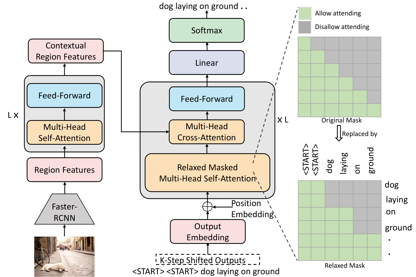
Given the image region features extracted by a pre-trained Faster-RCNN model Ren et al. 2015; Anderson et al. 2018, SATIC aims to generate a caption in a semi-autoregressive manner. The architecture of SATIC model is shown in Figure 2, which consists of an encoder and decoder.
Image Features Encoder.
The encoder takes the image region features as inputs and outputs the contextual region features. It consists of a stack of identical layers. Each layer has two sublayers. The first is a multi-head self-attention sublayer and the second is a position-wise feed-forward sublayer. Both sublayers are followed by residual connection He et al. 2016 and layer normalization Ba et al. 2016 operations for stable training. Multi-head self-attention builds on scaled dot-product attention, which operates on a query Q, key K and value V as:
| (3) |
where is the dimension of the key. Multi-head self-attention firstly projects the queries, keys and values times with different learned linear projections and then computes scaled dot-product attention for each one. After that, it concatenates the results and projects them with another learned linear projection:
| (4) | |||
| (5) |
where , and . The self-attention in the encoder performs attention over itself, i.e., (), which is the image region features in the first layer. After a multi-head self-attention sublayer, the position-wise feed-forward sublayer (FFN) is applied to each position separately and identically:
| (6) |
where , , and are learnable parameter matrices.
Captioning Decoder.
The decoder takes contextual region features and previous word embedding features as input and outputs predicted words probability. To make use of order information, position encodings Vaswani et al. 2017 are added to word embedding features. Different from original autoregressive Transformer model, which outputs a word at each step, SATIC takes a group of words as input and outputs a group of words at each step during decoding. Each group contains consecutive words. At the beginning of decoding, we feed the model with START symbols to predicate and then are fed as input to predicate in parallel. This process will continue until the end of sentence. An intuitive example is shown in the middle of Figure 1 with . The decoder also consists of identical layers and each layer has three sublayers: a relaxed masked multi-head self-attention sublayer, multi-head cross-attention sublayer and a position-wise feed-forward sublayer. Residual connection and layer normalization are also applied after each sublayer. The multi-head cross-attention is similar with the multi-head self-attention mentioned above except that the key and value are now contextual region features and the query is the output of its last sublayer. It is particularly worth emphasizing that original masked multi-head attention is replaced with the relaxed masked multi-head self-attention. The only difference between the two sublayer lie in the self-attention mask. Specifically, the original lower triangular matrix mask is now replaced by the relaxed mask. Formally, given the caption length and group size , the relaxed mask is defined as:
| (7) |
where and denotes floor operation. An intuitive example is shown in the right of Figure 2, where and . As a consequence, the scaled dot-product attention in relaxed masked multi-head self-attention module is modified to:
| (8) |
.
4.2 Training
Since SATIC model keeps the autoregressive property in global and the non-autoregressive property in local, it gets the best of both world and the conditional probability can be formulated as:
| (9) |
where represents the groups before -th group and except for the last group which may have less than words. If the length of padded word sequence can’t be divided by , remaining words only keep in output but not in input. Comparing Equation 1 and Equation 2 with Equation 9, we can find that autoregressive and non-autoregressive image captioning models are special cases of SATIC model when and respectively. At the first training stage, we optimize the model by minimizing cross-entropy loss:
| (10) | ||||
At the second training stage, we finetune the model using self-critical training Rennie et al. 2017 and the gradient can be expressed as:
| (11) |
where is the CIDEr Vedantam et al. 2015 score function, and is the baseline score. We adopt the baseline score proposed in Luo 2020, where the baseline score is defined as the average reward of the rest samples rather than original greedy decoding reward. We sample captions for each image and is the -th sampled caption.
| Models | BLEU-1 | BLEU-4 | METEOR | ROUGE | SPICE | CIDEr | Latency | Speedup |
| Autoregressive models | ||||||||
| NIC-v2 Vinyals et al. 2015 | / | 32.1 | 25.7 | / | / | 99.8 | / | / |
| Up-Down Anderson et al. 2018 | 79.8 | 36.3 | 27.7 | 56.9 | 21.4 | 120.1 | / | / |
| AOANet Huang et al. 2019 | 80.2 | 38.9 | 29.2 | 58.8 | 22.4 | 129.8 | / | / |
| M2-T† Cornia et al. 2020 | 80.8 | 39.1 | 29.2 | 58.6 | 22.6 | 131.2 | / | / |
| AIC† () | 80.5 | 38.8 | 29.0 | 58.7 | 22.7 | 128.0 | 135ms | 2.25 |
| AIC† () | 80.8 | 39.1 | 29.1 | 58.8 | 22.9 | 129.7 | 304ms | 1.00 |
| Non-autoregressive models | ||||||||
| MNIC† Gao et al. 2019 | 75.4 | 30.9 | 27.5 | 55.6 | 21.0 | 108.1 | - | 2.80 |
| FNIC †Fei 2019 | / | 36.2 | 27.1 | 55.3 | 20.2 | 115.7 | - | 8.15 |
| MIR †Lee et al. 2018 | / | 32.5 | 27.2 | 55.4 | 20.6 | 109.5 | - | 1.56 |
| CMAL †Guo et al. 2020 | 80.3 | 37.3 | 28.1 | 58.0 | 21.8 | 124.0 | - | 13.90 |
| Partially Non-autoregressive models | ||||||||
| PNAIC(K=2) †Fei 2021 | 80.4 | 38.3 | 29.0 | 58.4 | 22.2 | 129.4 | - | 2.17 |
| PNAIC(K=5) †Fei 2021 | 80.3 | 38.1 | 28.7 | 58.3 | 22.0 | 128.5 | - | 3.59 |
| PNAIC(K=10) †Fei 2021 | 79.9 | 37.5 | 28.2 | 58.0 | 21.8 | 125.2 | - | 5.43 |
| SATIC(K=2, bw=3) † | 80.8 | 38.4 | 28.8 | 58.5 | 22.7 | 129.0 | 184ms | 1.65 |
| SATIC(K=2, bw=1) † | 80.7 | 38.3 | 28.8 | 58.5 | 22.7 | 128.8 | 76ms | 4.0 |
| SATIC(K=4, bw=3) † | 80.7 | 38.1 | 28.6 | 58.4 | 22.4 | 127.4 | 127ms | 2.39 |
| SATIC(K=4, bw=1) † | 80.6 | 37.9 | 28.6 | 58.3 | 22.3 | 127.2 | 46ms | 6.61 |
| SATIC(K=6, bw=3) † | 80.6 | 37.6 | 28.3 | 58.1 | 22.1 | 126.2 | 119ms | 2.55 |
| SATIC(K=6, bw=1) † | 80.6 | 37.6 | 28.3 | 58.1 | 22.2 | 126.2 | 35ms | 8.69 |
5 Experiments
5.1 Dataset and Evaluation Metrics.
MSCOCO Chen et al. 2015 is the widely used benchmark for image captioning. We use the ‘Karpathy’ splits Karpathy and Feifei 2015 for offline experiments. This split contains training images, validation images and testing images. Each image has captions. We also upload generated captions of MSCOCO official testing set, which contains images for online evaluation. We evaluate the quality of captions by standard metricsChen et al. 2015 , including BLEU-1/4, METEOR, ROUGE, SPICE, and CIDEr, denoted as B1/4, M, R, S, and C, respectively.
5.2 Implementation Details.
Each image is represented as to region features with dimensions extracted by Anderson et al. Anderson et al. 2018. The dictionary is built by dropping the words that occur less than times and ends up with a vocabulary of . Captions longer than words are truncated. Both our SATIC model and autoregressive image captioning base model (AIC) almost follow the same model hyper-parameters setting as in Vaswani et al. 2017 (). As for the training process, we train AIC under cross entropy loss for 15 epochs with a mini batch size of 10, and optimizer in Vaswani et al. 2017 is used with a learning rate initialized by 5e-4 and the warmup step is set to . We increase the scheduled sampling probability by 0.05 every 5 epochs. We then optimize the CIDEr score with self-critical training for another 25 epochs with an initial learning rate of 1e-5. Our best SATIC model shares the same training script with AIC model except that we first initialize the weights (weight-init) of SATIC model with the pre-trained AIC model and replace the ground truth captions in the training set with sequence knowledge (SeqKD) Kim and Rush 2016; Gu et al. 2017a results of AIC model with beam size during cross entropy training stage. Unless otherwise indicate, latency represents the time to decode a single image without batching averaged over the whole test split, and is tested on a NVIDIA Tesla T4 GPU. The time for image feature extraction is not included in latency.
| Model | BLEU-1 | BLEU-2 | BLEU-3 | BLEU-4 | METEOR | ROUGE-L | CIDEr-D | |||||||
| c5 | c40 | c5 | c40 | c5 | c40 | c5 | c40 | c5 | c40 | c5 | c40 | c5 | c40 | |
| Up-Down∗ Anderson et al. 2018 | 80.2 | 95.2 | 64.1 | 88.8 | 49.1 | 79.4 | 36.9 | 68.5 | 27.6 | 36.7 | 57.1 | 72.4 | 117.9 | 120.5 |
| AOANet Huang et al. 2019 | 81.0 | 95.0 | 65.8 | 89.6 | 51.4 | 81.3 | 39.4 | 71.2 | 29.1 | 38.5 | 58.9 | 74.5 | 126.9 | 129.6 |
| M2-T∗ Cornia et al. 2020 | 81.6 | 96.0 | 66.4 | 90.8 | 51.8 | 82.7 | 39.7 | 72.8 | 29.4 | 39.0 | 59.2 | 74.8 | 129.3 | 132.1 |
| CMAL Guo et al. 2020 | 79.8 | 94.3 | 63.8 | 87.2 | 48.8 | 77.2 | 36.8 | 66.1 | 27.9 | 36.4 | 57.6 | 72.0 | 119.3 | 121.2 |
| PNAIC Fei 2021 | 80.1 | 94.4 | 64.0 | 88.1 | 49.2 | 78.5 | 36.9 | 68.2 | 27.8 | 36.4 | 57.6 | 72.2 | 121.6 | 122.0 |
| SATIC (K=4) | 80.3 | 94.5 | 64.4 | 87.9 | 49.2 | 78.2 | 37.0 | 67.2 | 28.2 | 37.0 | 57.8 | 72.6 | 121.5 | 124.1 |
5.3 Quantitative Results
In this section, we will analyse SATIC in detail by answering following questions.
How does SATIC perform compared with state-of-the-art models?
We compare the performance of SATIC with other state-of-the-art autoregressive models, non-autoregressive models and a partially non-autoregressive model. Among the autoregressive models, M2-T and AIC are based on similar Transformer architecture, while others are based on LSTM Hochreiter and Schmidhuber 1997. For non-autoregressive models, MNIC and MIR adopts an iterative refinement strategy, FNIC orders words detected in the image with an RNN and CMAL optimizes sentence-level reward. PNAIC is a partially non-autoregressive model which divides sentence into word groups and the groups are generated parallelly in global while each word in group is predicted from left to right. As shown in Table 1, SATIC achieves comparable performance with state-of-the-art autoregressive models but with significant speedup. When , SATIC achieves about speedup while the caption quality only degrades slightly compared with its autoregressive counterpart AIC model. Compared with non-autoregressive models , SATIC obviously achieves a better trade-off between quality and speed by outperforming all the non-autoregressive models except CMAL in speedup metric. Compared with most similar partially non-autoregressive model PNAIC, SATIC achieves similar speedup and caption evaluation results. It is worth nothing that SATIC outperforms PNAIC on SPICE metric, which concerns more on semantic propositional content. What’s more, the training of SATIC is more easy and straightforward than PNAIC. Overall, SATIC achieves a better trade-off between quality, speed and easy training. We also show the results of online MSCOCO evaluation in Table 2.
What is the effect of group size ?
We test three different setting of the group size, i.e. . From the bottom of Table 1, we can observe that a larger brings more significant speedup while the caption quality degrades moderately. For example, the decoding speed increases about while the CIDEr score drops about when grows from to , and drops no more than when grows further to . This is intuitive since is the indicator of parallelization and also indicates that SATIC model is relatively stable to and has a good trade-off between speed and quality.
Can SATIC benefit from beam search?
From the bottom of Table 1, we can also find that SATIC benefits little (CIDEr score only increases ) from beam search compared with its autoregressive counterpart AIC (CIDEr score increases ) after self-critical training. There are two possibilities, the one is self-critical training make its output probability concentrated and the other one is SATIC can not benefit from beam search. To investigate whether SATIC can benefit from beam search, we test its output just after cross entropy training with different beam search width. From Table 3, we can observe that SATIC model can still benefit from beam search and there are two interesting phenomena: 1) SATIC with too large benefits less from beam search and 2) the effect of beam search is larger when without weight initialization and sequence knowledge distillation. A plausible explanation is that long-distance dependence is hard to capture and sequence knowledge distillation decreases dependence among words.
| Models | bw | B1 | B4 | M | R | S | C |
| w/ weight-init and SeqKD: | |||||||
| K=2 | 1 | 79.3 | 36.2 | 28.2 | 57.4 | 22.1 | 121.5 |
| 3 | 80.0 | 37.3 | 28.4 | 57.8 | 22.3 | 123.9 | |
| K=4 | 1 | 77.3 | 32.9 | 27.0 | 56.0 | 20.5 | 111.0 |
| 3 | 78.0 | 34.4 | 27.2 | 56.5 | 20.9 | 114.5 | |
| K=6 | 1 | 77.3 | 33.3 | 26.7 | 56.0 | 20.4 | 110.3 |
| 3 | 77.2 | 33.7 | 26.6 | 56.1 | 20.4 | 110.7 | |
| w/o weight-init and SeqKD : | |||||||
| K=2 | 1 | 74.2 | 29.1 | 25.8 | 53.8 | 19.5 | 100.0 |
| 3 | 76.0 | 32.8 | 26.8 | 55.2 | 20.6 | 107.2 | |
| K=4 | 1 | 65.8 | 17.0 | 21.8 | 48.3 | 16.1 | 73.3 |
| 3 | 69.7 | 20.9 | 22.7 | 50.2 | 16.6 | 79.6 | |
| K=6 | 1 | 67.6 | 17.6 | 21.3 | 48.6 | 15.2 | 73.5 |
| 3 | 68.8 | 19.1 | 21.6 | 49.6 | 15.5 | 76.3 |
What is the effect of sequence knowledge distillation and weight initialization?
We further investigate the effect of sequence knowledge distillation and weight initialization and results are shown in Table 4. We can find that sequence knowledge distillation plays an important role in both XE and SC training stages and the effect is more significant in XE stage . Basically, the larger the is, the more obvious the effect is. This is intuitive since the ability of SATIC model to capture conditional probability is undermined when grows and sequence knowledge distillation compensates for this by reducing the complexity of data sets. SC can also alleviate sentence-level inconsistency by providing sentence-level reward. In addition to accelerate convergence, we can find that weight initialization slightly improves the caption quality when is small but has important impact when is large.
What is the effect of batch size on latency?
Above latency is measured with batch size set to . However, there may be multiple requests at once in real application. So, we further investigate the latency under various batch size setting. From Table 5, we can find that SATIC can basically accelerate decoding even under large batch size. We can also observe that the speedup is decline as batch size increases. This indicates that non-gpu program becomes a bottleneck when the runtime of gpu program is negligible.
| Models | XE | SC | ||||||||
| B1 | B4 | M | S | C | B1 | B4 | M | S | C | |
| K=2: | ||||||||||
| Base | 74.2 | 29.1 | 25.8 | 19.5 | 100.0 | 80.3 | 37.6 | 28.4 | 22.0 | 123.7 |
| +SeqKD | 78.8 | 36.0 | 28.0 | 21.8 | 120.4 | 80.5 | 38.4 | 28.7 | 22.6 | 128.1 |
| +Weight-init | 79.3 | 36.2 | 28.2 | 22.1 | 121.5 | 80.7 | 38.3 | 28.8 | 22.7 | 128.8 |
| K=4: | ||||||||||
| Base | 65.8 | 17.0 | 21.8 | 16.1 | 73.3 | 79.8 | 35.3 | 27.3 | 20.9 | 119.5 |
| +SeqKD | 69.5 | 22.2 | 23.0 | 16.7 | 85.5 | 80.4 | 37.5 | 28.3 | 22.2 | 126.0 |
| +Weight-init | 77.3 | 32.9 | 27.0 | 20.5 | 111.0 | 80.6 | 37.9 | 28.6 | 22.3 | 127.2 |
| K=6: | ||||||||||
| Base | 67.6 | 17.6 | 21.3 | 15.2 | 73.5 | 79.2 | 32.2 | 26.7 | 20.4 | 116.1 |
| +SeqKD | 73.2 | 27.0 | 24.6 | 18.1 | 96.3 | 79.9 | 37.0 | 28.0 | 21.6 | 123.9 |
| +Weight-init | 77.3 | 33.3 | 26.7 | 20.4 | 110.3 | 80.6 | 37.6 | 28.3 | 22.2 | 126.2 |
| Model | b=1 | b=8 | b=16 | b=32 | b=64 |
| Transformer | 135ms | 22ms | 13ms | 11ms | 10ms |
| SATIC, =2 | 76ms | 13ms | 8ms | 7ms | 7ms |
| SATIC, =4 | 46ms | 8ms | 6ms | 5ms | 5ms |
| SATIC, =6 | 35ms | 7ms | 5ms | 5ms | 5ms |
5.4 Qualitative Results
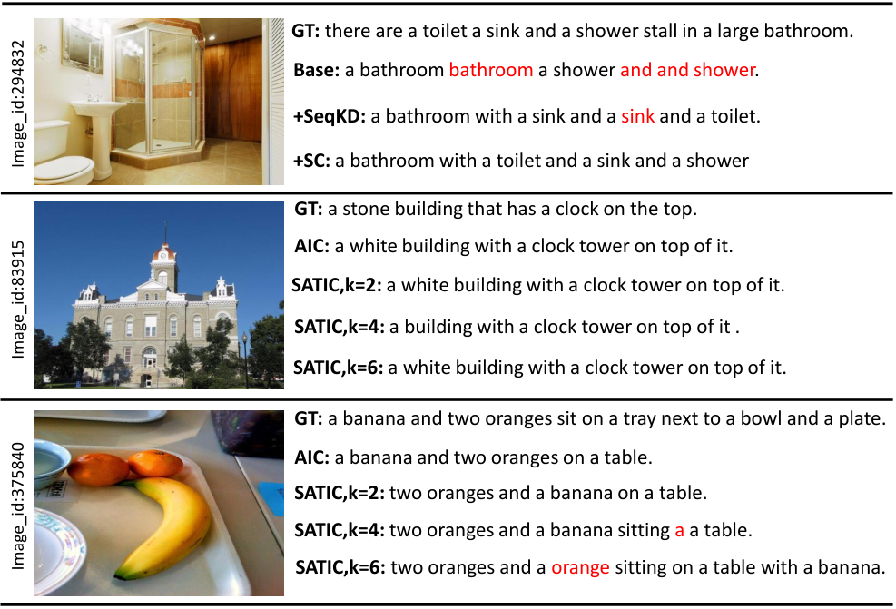
We present three examples of generated image captions in Figure 3. From the top example, we can intuitively understand the effect of sequence knowledge distillation (SeqKD) and self-crical training (SC) in reducing repeated words and incomplete content. In general, the final SATIC models with different group size can generate fluent captions, as shown in the middle example. Nevertheless, repeated words and incomplete content issues still exist, especially when is large. As shown in the bottom example, ‘a’ and ‘orange’ are repeated words and ‘tray’,‘bowl’ are missing.
6 Conclusion
In this paper, we introduce a semi-autoregressive model for image captioning (dubbed as SATIC), which keeps the autoregressive property in global and non-autoregressive property in local. We conduct substantial experiments on MSCOCO image captioning benchmark to better understand the effect of each component. Overall, SATIC achieves a better trade-off between speed,quality and easy training.
References
- Anderson et al. [2018] Peter Anderson, Xiaodong He, Chris Buehler, Damien Teney, Mark Johnson, Stephen Gould, and Lei Zhang. Bottom-up and top-down attention for image captioning and visual question answering. In CVPR, 2018.
- Ba et al. [2016] Jimmy Lei Ba, Jamie Ryan Kiros, and Geoffrey E Hinton. Layer normalization. arXiv, 2016.
- Chen et al. [2015] Xinlei Chen, Hao Fang, Tsung-Yi Lin, Ramakrishna Vedantam, Saurabh Gupta, Piotr Dollár, and C Lawrence Zitnick. Microsoft coco captions: Data collection and evaluation server. arXiv, 2015.
- Cornia et al. [2020] Marcella Cornia, Matteo Stefanini, Lorenzo Baraldi, and Rita Cucchiara. Meshed-memory transformer for image captioning. In CVPR, 2020.
- Fei [2019] Zheng-cong Fei. Fast image caption generation with position alignment. arXiv, 2019.
- Fei [2021] Zhengcong Fei. Partially non-autoregressive image captioning. In AAAI, 2021.
- Gao et al. [2019] Junlong Gao, Xi Meng, Shiqi Wang, Xia Li, Shanshe Wang, Siwei Ma, and Wen Gao. Masked non-autoregressive image captioning. arXiv, 2019.
- Gu et al. [2017a] Jiatao Gu, James Bradbury, Caiming Xiong, Victor OK Li, and Richard Socher. Non-autoregressive neural machine translation. arXiv, 2017.
- Gu et al. [2017b] Jiuxiang Gu, Gang Wang, Jianfei Cai, and Tsuhan Chen. An empirical study of language cnn for image captioning. In ICCV, 2017.
- Guo et al. [2019] Junliang Guo, Xu Tan, Di He, Tao Qin, Linli Xu, and Tie-Yan Liu. Non-autoregressive neural machine translation with enhanced decoder input. In AAAI, 2019.
- Guo et al. [2020] Longteng Guo, Jing Liu, Xinxin Zhu, Xingjian He, Jie Jiang, and Hanqing Lu. Non-autoregressive image captioning with counterfactuals-critical multi-agent learning. arXiv, 2020.
- He et al. [2016] Kaiming He, Xiangyu Zhang, Shaoqing Ren, and Jian Sun. Deep residual learning for image recognition. CVPR, 2016.
- Hochreiter and Schmidhuber [1997] Sepp Hochreiter and Jürgen Schmidhuber. Long short-term memory. Neural computation, 1997.
- Huang et al. [2019] Lun Huang, Wenmin Wang, Jie Chen, and Xiao-Yong Wei. Attention on attention for image captioning. In ICCV, 2019.
- Jiang et al. [2020] Huaizu Jiang, Ishan Misra, Marcus Rohrbach, Erik Learned-Miller, and Xinlei Chen. In defense of grid features for visual question answering. In CVPR, 2020.
- Karpathy and Feifei [2015] Andrej Karpathy and Li Feifei. Deep visual-semantic alignments for generating image descriptions. CVPR, 2015.
- Kim and Rush [2016] Yoon Kim and Alexander M Rush. Sequence-level knowledge distillation. arXiv, 2016.
- Lee et al. [2018] Jason Lee, Elman Mansimov, and Kyunghyun Cho. Deterministic non-autoregressive neural sequence modeling by iterative refinement. arXiv, 2018.
- Li et al. [2020] Xiujun Li, Xi Yin, Chunyuan Li, Pengchuan Zhang, Xiaowei Hu, Lei Zhang, Lijuan Wang, Houdong Hu, Li Dong, Furu Wei, et al. Oscar: Object-semantics aligned pre-training for vision-language tasks. In ECCV, 2020.
- Luo [2020] Ruotian Luo. A better variant of self-critical sequence training. arXiv, 2020.
- Pan et al. [2020] Yingwei Pan, Ting Yao, Yehao Li, and Tao Mei. X-linear attention networks for image captioning. In CVPR, 2020.
- Ran et al. [2020] Qiu Ran, Yankai Lin, Peng Li, and Jie Zhou. Learning to recover from multi-modality errors for non-autoregressive neural machine translation. arXiv, 2020.
- Ren et al. [2015] Shaoqing Ren, Kaiming He, Ross Girshick, and Jian Sun. Faster r-cnn: Towards real-time object detection with region proposal networks. In NeurIPS, 2015.
- Rennie et al. [2017] Steven J Rennie, Etienne Marcheret, Youssef Mroueh, Jerret Ross, and Vaibhava Goel. Self-critical sequence training for image captioning. In CVPR, 2017.
- Vaswani et al. [2017] Ashish Vaswani, Noam Shazeer, Niki Parmar, Jakob Uszkoreit, Llion Jones, Aidan N Gomez, Łukasz Kaiser, and Illia Polosukhin. Attention is all you need. In NeurIPS, 2017.
- Vedantam et al. [2015] Ramakrishna Vedantam, C. Lawrence Zitnick, and Devi Parikh. Cider: Consensus-based image description evaluation. Computer Science, 2015.
- Vinyals et al. [2015] Oriol Vinyals, Alexander Toshev, Samy Bengio, and Dumitru Erhan. Show and tell: A neural image caption generator. In CVPR, 2015.
- Wang et al. [2018] Chunqi Wang, Ji Zhang, and Haiqing Chen. Semi-autoregressive neural machine translation. arXiv, 2018.
- Wang et al. [2019] Yiren Wang, Fei Tian, Di He, Tao Qin, ChengXiang Zhai, and Tie-Yan Liu. Non-autoregressive machine translation with auxiliary regularization. arXiv, 2019.
- Xu et al. [2015] Kelvin Xu, Jimmy Lei Ba, Ryan Kiros, Kyunghyun Cho, Aaron C Courville, Ruslan Salakhudinov, Rich Zemel, and Yoshua Bengio. Show, attend and tell: Neural image caption generation with visual attention. ICML, 2015.
- Yang et al. [2019] Xu Yang, Kaihua Tang, Hanwang Zhang, and Jianfei Cai. Auto-encoding scene graphs for image captioning. In CVPR, 2019.
- Yang et al. [2021] Bang Yang, Yuexian Zou, Fenglin Liu, and Can Zhang. Non-autoregressive coarse-to-fine video captioning. In AAAI, 2021.
- Yao et al. [2018] Ting Yao, Yingwei Pan, Yehao Li, and Tao Mei. Exploring visual relationship for image captioning. In ECCV, 2018.
- Zhou et al. [2020a] Luowei Zhou, Hamid Palangi, Lei Zhang, Houdong Hu, Jason Corso, and Jianfeng Gao. Unified vision-language pre-training for image captioning and vqa. In AAAI, 2020.
- Zhou et al. [2020b] Yuanen Zhou, Meng Wang, Daqing Liu, Zhenzhen Hu, and Hanwang Zhang. More grounded image captioning by distilling image-text matching model. In CVPR, 2020.