State Estimation with Model Reduction and Shape Variability. Application to biomedical problems.
Abstract
We develop a mathematical and numerical framework to solve state estimation problems for applications that present variations in the shape of the spatial domain. This situation arises typically in a biomedical context where inverse problems are posed on certain organs or portions of the body which inevitably involve morphological variations. If one wants to provide fast reconstruction methods, the algorithms must take into account the geometric variability. We develop and analyze a method which allows to take this variability into account without needing any a priori knowledge on a parametrization of the geometrical variations. For this, we rely on morphometric techniques involving Multidimensional Scaling, and couple them with reconstruction algorithms that make use of linear subspaces pre-computed on a database of geometries. We prove the potential of the method on a synthetic test problem inspired from the reconstruction of blood flows and quantities of medical interest with Doppler ultrasound imaging.
Key words. Inverse problems, Shape variability, Non-parametric domains, Model reduction, Multi-dimensional scaling, Variational data assimilation.
AMS subject classifications. 65D99,76Z05,35R30
1 Introduction
1.1 Scientific setting and contribution
A central task to address numerous applications in science and engineering is the problem of repeatedly evaluating the output of an expensive forward model for many instances of input parameter values. Such settings include the numerical solution of parametric Partial Differential Equations (PDEs) for different values of the parameter, and, more generally, the multiple evaluation of input-output maps defined by computer models. In the case of parametric PDEs, this task is usually known as model order reduction (MOR). To guide the subsequent discussion, consider the prototypical parametric PDE,
where is a differential operator and is a vector of parameters that describes physical properties. We assume can take values from given compact set . is an open bounded set which denotes the domain of the independent variables in the PDE. It usually refers to space but it is not limited to that meaning, and it could also refer to more elaborate sets of variables such as time, momentum, or other physical variables. For every , we assume that the PDE has a unique solution on a Hilbert space of real-valued functions on .
The main task of model reduction is to build a fast parameter-to-solution map that accurately approximates the set of PDE solutions
| (1.1) |
when the parameter varies in . This set is sometimes referred to as the solution manifold. Classically, the bottom line of most strategies has been based on approximating with linear spaces from , but developing nonlinear approximation strategies to overcome certain known bottlenecks is a subject of very active research (for some examples, we refer to [1, 2, 3, 4]).
Most linear and nonlinear model reduction methods are built for applications when is a fixed domain, but in numerous situations can actually vary, and this raises interesting challenges. This question about geometric variability is by far not new in model reduction, and numerous algorithms and works have been proposed to address it. Most existing strategies crucially rely on assuming that the family of domains is generated by a known (and easy) parametrization. The problem about the geometric variabillity can then be addressed by computing a reduced model on a reference domain, which is then mapped to a new target geometry in a relatively easy manner thanks to the assumption of an explicit parametrization of the geometries. The type of applications in which these developments have mostly been considered are connected to forward problems where the value of and of the geometrical parameters of the geometry are given as an input to approximate .
This paper is a contribution to go beyond this setting on several fronts:
- •
Nonparametric geometries: We propose a method where the family of geometries is nonparametric. In other words, we do not assume a known parametrization of the domains. This is particularly relevant in certain applications such as biomedical problems where the domain is often given by the shape of a certain organ which inevitably presents morphological variations. These variations are difficult to parametrize, and, in fact, information on the family of geometries is often given by a collection of images of each patient’s organ.
- •
Forward and inverse problems: We explain how the method can be applied not only for the purpose of forward problems, but also for solving inverse state estimation problems in a reasonable amount of time. In the inverse problem setting, we do not get the value of the parameters . Instead, we are given measurement observations (whose nature varies depending on the application). This makes inverse problems ill posed, and it adds an extra layer of difficulty to the problem. Although the developed method is general and could be used with both linear and nonlinear types of methods, the presentation in this paper focuses mostly on linear methods, and results about the benefits of using nonlinear strategies is left for future work. As such, the main method which we use for forward reduced modeling is based on (linear) Principal Component Analysis (PCA), and we adapt the so-called Parametrised Background Data Weak (PBDW) approach for inverse state estimation. This algorithm was proposed in [5] and analyzed in subsequent papers such as [6, 7, 8, 9, 10, 11, 12].
- •
Enhanced use of database information: To work in a nonparametric geometrical setting, our approach requires to have a collection of domains and solution manifolds with their associated forward reduced models to carry out a learning phase. We then introduce a notion of measuring distances between manifold sets on different domains . This allows us to find the geometry from the database with the closest physics to a new given target geometry. The precomputed reduced model of the closest neighbor is then transported to the target geometry to solve forward or inverse problem queries. The use of a database of geometries is a salient novelty with respect to most approaches, and it allows to better take into account potential variations of the physics that could be induced by domain changes. Working with a database is however not fully new, though. It was proposed in [13] which is probably the contribution from the literature that shares more points of contact with the present work. We discuss the main novelties and similarities in Section 1.3, where we also give an overview of previous works.
Our work was motivated by applications in biomedical engineering. The prototypical yet fundamental situation regards the clinical applications in which non-invasive measurements (typically acquired by medical imaging) are exploited in order to infer non-observable mechanical or physiological properties, or to perform state estimation. The time constraints of the clinical applications clearly motivate and justify the use of model order reduction, and inverse state estimation algorithms based on them. However, the inter-patient variability is often very large and manifests itself also in terms of anatomy, hence the geometrical variability. This points towards working with a database of geometries obtained from previous patient’s examinations in order to be able to examine a wide range of patients. On the data set of geometries, we precompute linear (or nonlinear) reduced models, and then re-use this information for the examination in real time of a new given patient which comes with a new morphology.
1.2 Organization of the paper
At the end of Section 1.3 we give an overview of previous works on model reduction in variable geometries. In Section 2 we present the context of inverse state estimation and the methods we use in the present work. In Section 3 we detail the strategy we adopt in order to deal with variable domain geometries. In Section 4 we propose an error analysis for the state estimation problem. In section 5 we describe in detail how the different steps of the procedure are practically implemented and we conclude by presenting a numerical experiment to assess the method. The example takes inspiration from the reconstruction of blood flows with Doppler ultrasound images.
1.3 Previous works on model reduction with variable geometries
The topic of working with variable geometries is common to several fields of research such as shape optimisation ([14, 15, 16]), inverse scattering problems ([17]), geometry morphometrics ([18, 19]). In the field of model order reduction, the main challenge stems from the fact that, usually, one needs to define in which linear reduced space the computations are done, and this depends on the domain. Numerous works have studied this issue in the literature. A first example is provided in [20], in which a reduced-element method is devised, to take advantage of domain decomposition techniques and adapt to various potentially deformed domains. An important class of methods consists in mapping the domains into a same reference configuration and write the equations in this latter. In [21], the authors consider the set of transformations with affine parametrisation and their effect on the inf-sup stability for a reduced-basis formulation of the Stokes problem. In [22], the computational domain is deformed thanks to an elastic displacement and the non-affine dependence of the equations on the domain is tackled by using a matrix-DEIM approach. A similar approach is proposed in [23] to efficiently reduce the computational cost of parametrised fluid models. In [24], an isogeometric analysis framework is used to deal with the domain parametrisation and build a reduced-basis method to speed up shape optimisation problems. A similar approach is proposed in [25]. In [26], the parametrisation of the domain (obtained by considering non-uniform rational B-splines [27])) is incorporated as extra-coordinate in a Progressive Generalised Decomposition (PGD) method. In [28], a free-form deformation method is coupled to Proper Orthogonal Decomposition (POD, see e.g. [29, 30, 31]) in the context of shape optimisation in aerodynamics. In [32], instead of mapping the domains into a common reference configuration, the shifted boundary method is applied to deal with the geometry parametrisation. By doing so, we avoid the changes of coordinate; to deal with the intrinsic non-linearity, the authors propose to use the GNAT method or the gappy-POD. In [33], an hyper-reduction framework is used to deal with non-parametrised geometrical variations of the domain in the context of fluid-mechanics. In [34], a reduced-basis formulation is proposed to deal with a cut-FEM embedding method. In [35], the reduced-basis functions are defined on an average-deformed configuration in order to speed up finite volume computations for fluid models with variable geometries. In [36], the authors consider the problem of the parametrisation of interfaces in the context of fluid-structure interaction problems. In [37], the reduced-basis method is used to efficiently solve the Maxwell equations to speed up the design of semiconductors. In [38, 39] and other recent works, the authors consider the problem of registration applied to model reduction: by suitably transforming the domain we can achieve the reduction efficiency. Numerous applications including geometry reduction can take advantage of such techniques.
To the best of our knowledge, the work which shares more similarities with the present contribution is [13]. In that work, a set of realistic patient template geometries is built without knowing the underlying, potentially high-dimensional, parametrisation. The authors then construct the reduced-order model on a reference geometry computed as the average of the available templates (in the sense defined in the paper). A set of transformations allow to map fields between the geometries and the average geometry. The two main differences with respect to the present work are the following: we construct a reduced-order method in view of performing the reconstruction given some observable so, instead of constructing an atlas based solely on geometric information, we construct a set of templates based also on the physics of the problem we are considering. In order to solve the state estimation problem in a reduced way, we adapt the Parametrised Background Data Weak approach [5].
2 Multi-Domain State Estimation: Problem Setting
In the following, the terms geometry, spatial domain, and shape will be used interchangeably whenever there is no ambiguity.
2.1 State estimation on a given domain
Let be a fixed given domain of with dimension , and let be a Hilbert space defined over . The space is endowed with an inner product and induced norm . The choice of must be relevant for the problem under consideration, and typical options are , or some Reproducing Kernel Hilbert Space.
Our goal is to recover an unknown function from possibly noisy measurement observations
| (2.1) |
where the are linearly independent linear forms from and the are unknown measurement errors. In the following, for the sake of simplicity, we will assume that there is no noise () but the main methodology which we develop could easily be extended to deal with noisy measurements. In practical applications, each models a sensor device which is used to collect the measurement data . In the applications which we present in our numerical tests, the observations come in the form of an image and each models the response of the system on a given pixel. Figure 4 illustrates a complete synthetic image.
We denote by the Riesz representers of the . They are defined via the variational equation
Since the are linearly independent in , so are the in and they span an -dimensional space
When there is no measurement noise, knowing the observations is equivalent to knowing the orthogonal projection
| (2.2) |
In this setting, the task of recovering from the measurement observation can be viewed as building a recovery algorithm
such that is a good approximation of in the sense that is small.
Recovering from the measurements is a very ill-posed problem since is generally a space of very high or infinite dimension so, in general, there are infinitely many such that . It is thus necessary to add some a priori information on in order to recover the state up to a guaranteed accuracy. In the following, we work in the setting where is a solution to some parameter-dependent PDE of the general form
where is a differential operator and is a vector of parameters that describes some physical property and lives in a given set . For every , we assume that the PDE has a unique solution . Therefore, our prior on is that it belongs to the set
| (2.3) |
which is sometimes referred to as the solution manifold.
Performance Benchmarks:
The quality of a recovery mapping is usually quantified in two ways:
- •
If the sole prior information is that belongs to the manifold , the performance is usually measured by the worst case reconstruction error
(2.4) - •
In some cases is described by a probability distribution on supported on . This distribution is itself induced by a probability distribution on that is assumed to be known. When no information about the distribution is available, usually the uniform distribution is taken. In this Bayesian-type setting, the performance is usually measured in an average sense through the mean-square error
(2.5) and it naturally follows that .
PBDW as our practical algorithm:
In this work, we will reconstruct with the Parametrized-Background Data-Weak algorithm (PBDW, [5]). Other choices would of course be possible but the PBDW algorithm is relevant for the following reasons:
- •
Simplicity and Speed: It is easily implementable and it provides reconstructions in near-real time.
- •
- •
Extensions: If required, the algorithm can easily be extended to enhance its reconstruction performance (see [12, 40]). In particular, it is shown in [12] that piece-wise PBDW reconstruction strategy can deliver near-optimal reconstruction performance. The PBDW algorithm can also be easily adapted to accommodate noisy measurements (see [8, 10]) and some easy to implement extensions to mitigate the model error exist (in the following however, we assume the PDE model is perfect for the sake of simplicity).
Since the geometry of is generally complex, optimization tasks posed on are difficult (lack of convexity, high evaluation costs for different parameters). Therefore, instead of working with , PBDW works with a linear (or affine) subspace of reduced dimension which is expected to approximate the solution manifold well in the sense that the approximation error of the manifold,
| (2.6) |
decays rapidly if we increase the dimension . It has been proven in [41] that it is possible to find such hierarchies of spaces for certain manifolds coming from classes of elliptic and parabolic problems, and numerous strategies have been proposed to build the spaces in practice (see, e.g., [42, 43] for reduced basis techniques and [41, 44] for polynomial approximations in the variable).
Assuming that we are given a linear subspace with , the PBDW algorithm
gives for any a solution of
| (2.7) |
For any pair of closed subspaces of , we define as
| (2.8) |
The minimizer of (2.7) is unique as soon as and , which is an assumption to which we adhere in the following. In practice, solving problem (2.7) boils down to solving a linear least squares minimization problem. We refer, e.g., to [45, Appendix A] for details on how to compute it in practice.
We can prove that is a bounded linear map from to . In fact, it is a simple least squares problem whose cost is essentially . Therefore, if the dimension of the linear subspace is moderate, the reconstruction with (2.7) takes place in close to real-time.
The reconstruction error was first studied in [5] and further developed in [9]. In the later, the following result can be found: for any it holds
| (2.9) |
where we have omitted the dependency of the spaces on in order not to overload the notation, and we will keep omitting this dependency until the end of this section. Depending on whether is built to address the worst case or mean square error, the reconstruction performance over the whole manifold is bounded by
| (2.10) |
or
| (2.11) |
Note that can be understood as a stability constant. It can also be interpreted as the cosine of the angle between and . The error bounds involve the distance of to the space which provides slightly more accuracy than the linear subspace alone. This term is the reason why it is sometimes said that the method can correct model error to some extent. In the following, to ease the reading we will write errors only with the second type of bounds (2.11) that do not involve the correction part on .
An important observation is that for a fixed measurement space (which is the setting in our numerical tests), the error functions
reach a minimal value for a certain dimension and as the dimension varies from 1 to . This behavior is due to the trade-off between:
- •
the improvement of the approximation properties of as grows ( and as grows)
- •
the degradation of the stability of the algorithm, given here by the decrease of to 0 as . When , .
As a result, the best reconstruction performance with PBDW is given by
2.2 Obstructions when the spatial domain is not given a priori
The speed of the above reconstruction algorithm crucially relies on the fact that we have assumed that the spatial domain is given to us a priori. Thanks to this we can precompute the linear subspaces before the reconstruction takes place, and we only need to solve (2.7) during the reconstruction, which is a computation that can be done in near real-time. The offline computation of the reduced model should be seen as a training phase, and it can be computationally intensive and time-consuming for complex physical systems.
There are however cases in which we cannot assume that is given a priori. This situation typically arises in biomedical applications where state estimation needs to be performed on a certain part of the body for different patients which inevitably present morphological variations. In this case, given a new target geometry , one could of course generate and derive a linear subspace but this task would not be feasible in real-time, and the method would no be useful for real time decisions. To avoid this computational bottleneck, we propose a method to quickly build a space by using reduced models which have been pre-computed on a database of template geometries which we suppose to be available offline. The idea consists in finding the best reduced model from the template geometries, and then to transport it to the target geometry . Once this is done, we reconstruct with PBDW on the target geometry. The next section presents the details of our proposed strategy.
3 Proposed strategy for fast state estimation
We consider a set of spatial domains in . The set can potentially be infinite. An example for is the set of human carotid arteries or, more generally, the set of shapes of a certain organ. Our goal is to build a state estimation procedure that is fast for every geometry . For this, our approach is based on a learning phase that involves computations on a dataset of available template geometries. We next summarize the main steps. In section 4 we give an error analysis of the procedure and discuss the main sources of inaccuracy. Some steps involve certain routines which are introduced at an abstract level in this section and in the error analysis. In section 5, we explain how we have implemented them in practice, and how our theory justifies certain choices. Note however that since the procedure is general, other constructions can of course be considered for these building blocks.
4 Theoretical analysis of the reconstruction error
Suppose we are given a target geometry and that we want to reconstruct an unknown function from its observations . Suppose further that we fix a geometry and we transport the linear subspace space to the target geometry by applying . The goal of this section is to give an error bound on the reconstruction of with PBDW and using
as a linear subspace on . To ease the notation, we will use and to denote and respectively.
The results involve the following notion of Hausdorff distance between compact sets.
Definition 1.
For any two given compact sets and of a Hilbert space , the Hausdorff distance between and is defined as
4.1 An error bound based on
It is natural to expect that the reconstruction error will be of good quality if:
- •
the physical phenomena contained in the target manifold are well represented in some sense by the transported manifold , and if
- •
the linear subspace approximates with enough accuracy, and its quality is not degraded by the transport to the target geometry.
Theorem 4.1 formalises and quantifies this intuition under the following assumptions:
- 1.
In the template geometry , the accuracy of the template linear subspace is bounded by
(H1) for some .
- 2.
The Hausdorff distance between and is bounded by
(H2) for some . Note that couples the physics, the geometry and the transport between and . The bound on this term expresses the fact that the physics in the target domain , expressed via the manifold , should be well represented when we transport the physics from to . The value of could of course be large depending on the type of physics, geometries, and transport.
- 3.
We finally need two technical assumptions on the transport maps and :
- (a)
is Hölder continuous, namely there exists and such that
(H3) - (b)
There exists such that
(H4)
- (a)
Theorem 4.1.
Let be a template geometry and let be a target function to estimate from the observations . If we reconstruct with PBDW using
then the reconstruction error is bounded by
| (4.1) |
If the assumptions (H1) to (H4) hold, then the reconstruction error over the whole manifold is bounded by
| (4.2) |
Suboptimal bounds for are
| (4.3) | ||||
| (4.4) |
where the constant is the one given in assumption (H3).
Proof.
In this proof, all norms will be related to the space defined on the target geometry . Let . By (2.9), we have
| (4.5) |
which is the first inequality of the Theorem. We next bound in terms of quantities in the template geometry and the transport operators and . For this, let
and remark that
| (4.6) |
by assumption (H2).
By the triangle inequality and inequality (4.6),
| (4.7) | ||||
| (4.8) | ||||
| (4.9) |
and the error bound (4.2) follows by inserting (4.9) into (4.5).
We next bound as follows. For any , there exists such that . Therefore,
where we have added and subtracted , and applied the triangle inequality. By applying hypotheses (H3) and (H1), we can further bound the above inequality as
| (4.10) | ||||
| (4.11) |
which yields inequality (4.3). Inequality (4.4) follows from using (H3) and (H4) to bound in (4.11). Note that both inequalities (4.3) and (4.4) are suboptimal due to the construction of the bounds.
∎
Theorem 4.1 shows that several ingredients are required in order to obtain a good quality reconstruction in from a template geometry :
- •
The quality of the reduced basis in must be high so that is small enough.
- •
The transported manifold must be close the target manifold is the sense that is small enough.
- •
The transported space must have “a good alignment” with the observation space in the sense that the stability constant is bounded away from 0.
- •
Finally, the transport of the space with must approximate as well as possible the one with so that is small.
4.2 An alternative error bound based on subspace distances
The reconstruction error bound (4.2) given in Theorem 4.1 involves very natural quantities such as the Hausdorff distance between the target manifold and the transported one . The bound (4.2) may however be pessimistic in the sense that if is large, then the bound will not guarantee a high quality (because is large). In this scenario, the reconstruction may however still be of decent quality if the transported subspace does not deviate much compared to good quality reduced subspaces that one could compute in the target manifold .
Theorem 4.2 quantifies this argument. It is a perturbative result that expresses to what extent the reconstruction is degraded between working directly with a linear subspace and a transported subspace . The result involves the Hausdorff distance between the unit spheres of these two spaces, which we denote by and . The square of this distance can be written as
| (4.12) | ||||
where the Pythagorean identity () has been used.
Theorem 4.2.
Let be a linear subspace such that
| (4.13) | ||||
| (4.14) |
Let be a transported subspace from to such that
| (4.15) |
Then the reconstruction of with PBDW using is well-posed and the error is bounded by
If we use , the reconstruction is well posed if and only if
| (4.16) |
and the reconstruction error is bounded by
| (4.17) |
Proof.
Let . By direct application of (4.1), we have
| (4.18) |
By the triangle inequality and hypothesis (4.13) and (4.15),
| (4.19) |
We next prove that
| (4.20) |
Note that this automatically guarantees that the reconstruction using is well-posed since, by hypothesis (4.16), we have and therefore .
To prove (4.20), we start from the fact that
and, by Jensen’s inequality, we have that for any
| (4.21) |
Now, on the one hand,
| (4.22) |
On the other hand,
| (4.23) |
where we have used (4.14) to derive the last inequality. Thus inserting bounds (4.22) and (4.23) into (4.21), and setting , we derive
| (4.24) | ||||
| (4.25) | ||||
| (4.26) |
We can maximize the left-hand side over and minimize the right-hand side over . This yields
| (4.27) | ||||
| (4.28) | ||||
| (4.29) |
which is the proof to inequality (4.20). We derive the final result (4.17) by inserting bounds (4.20) and (4.19) into (4.5). ∎
From the error bound (4.17) from Theorem 4.2, it follows that if the transported subspace deviates from by a quantity of the order , then
for a relatively moderate constant . In this scenario, the reconstruction with the transported subspace is of the same quality as the one with the linear subspace (which we are avoiding to compute in order to speed-up the state estimation procedure).
5 Transport routine and the routine Best-Template
5.1 Computation of and
We next describe a practical way of mapping snapshots and subspaces from a given geometry to a target geometry . Our approach is based on building a one-to-one mapping between the two volumes and . It involves three steps:
- 1.
Surface matching: The task is to compute a map between and . For this, we use the so-called Large Deformation Diffeomorphic Metric Mapping (LDDMM, see for instance [46]) method. In practice, the output of this method is an invertible and smooth mapping between and an intermediate surface which is close to the target surface . The mapping is such that, if , then . The surface misfit between and is corrected in step 3 with an interpolation post-processing.
- 2.
Extrapolation of the surface map to the entire volume: We make a harmonic extension on and we find a displacement field such that
(5.1) (5.2) Note that if . We define the volumetric mapping
(5.3) (5.4) This map is invertible and . We further define the functional mapping
(5.5) (5.6) - 3.
Interpolation: Since in general , we add an interpolation operator , so that the final mapping is
(5.7) (5.8)
Note that the map may not exist if the spaces and are chosen of very different nature (very different regularity) or if certain physical quantities need to be preserved. One relevant example for fluid and biomedical applications is the space of divergence free fields where and . In this case, for any , we have but the function may not be divergence free. One remedy in this case is to add a post-process with the Piola transform. We therefore update the abstract definition of by adding a post-process mapping to allow this type of scenario,
| (5.9) | ||||
| (5.10) |
In our reconstruction method, we need to transport subspaces to subspaces of . Note that in general the image of by , defined as
is not a linear subspace of unless is a linear map. Due to this, given that in our approach we need to map subspaces into subspaces, we choose to define the image of with respect to a given basis of as
| (5.11) |
5.2 The Best-Template routine BT
The goal of this routine is to identify for each new target geometry which template geometry has the most appropriate linear subspace that we have to transport to .
Given a target geometry and a template geometry , the reconstruction error is bounded by (see (4.1))
| (5.12) |
where
| (5.13) |
Alternatively, if we study errors in the average sense,
| (5.14) |
with
| (5.15) |
Ideally, we would like to find the template that miminizes the upper bound (5.12) or (5.14), that is, find
where means or depending on the desired setting to study the errors. Note that this criterion depends on the observation space that we use for the reconstruction in , and there are two scenarios:
- •
We can use directly this criterion if we consider that is known with enough advance, and that we have enough time to compute for all . Note however that this is a very costly operation in general.
- •
There are settings in which a suboptimal criterion that does not involve but that is computationally faster might be required. One scenario in which this is the case is when one whishes to study several different observation spaces . Another scenario concerns applications in which one cannot assume that is known with enough advance. In such cases, the selection of the template geometry has to be performed in a reduced computational time in the online phase. This is the case of numerous biomedical problems which we are particularly targeting in our numerical experiments.
In the following, we present a strategy for the second, more challenging scenario. Our approach is based on Theorem 4.2. From bound (4.17) of that theorem, it follows that a strategy to find the best template is to minimize over the Hausdorff distance
| (5.16) |
between a good linear subspace (coming, for example, from forward reduced modeling) and the transported subspace . With this strategy, the output to select the best-template routine is thus
| (5.17) |
In order to perform this selection in real time, we need to estimate quickly the map
In our work, this is performed with a Multidimensional Scaling approach (MDS, see e.g. [47, 48, 49, 50]). We next describe the main steps.
Remark 5.1.
Working with the quantity (5.16) is theoretically justified by Theorem 4.2. Note that the theorem requires enough stability in the sense that (4.14) needs to be satisfied. This is taken as an assumption in the following development. In our numerical tests, this conditions is satisfied thanks to the quality of the data for the applications we focus on.
Step 1: Voxelize geometries:
To ease the manipulation and comparison between different domains, we work with voxelized descriptions of them involving a uniform grid mesh of cells. Therefore, instead of working with a given domain , we will actually manipulate vectors such that for all , the voxel entry is equal to the volume portion of the associated cell of the mesh. Ideally, the size of the grid mesh should be large enough in order to guarantee an isomorphism between the domains and their corresponding voxelizations .
The family of geometries is therefore replaced in practice by the voxelized representation,
Similarly,
As a result of the voxelization, we will alternatively write the manifold set of solutions as for all . Also, in practice we will construct a best template mapping of the form
Learning Phase – Step 1: MDS:
We consider the manifold set
Our goal is to find a low dimensional representation of using our database of templates,
For this, suppose that is equipped with a metric . The exact choice for will be specified later on. We then assemble the matrix of pairwise square distances between elements of ,
| (5.18) |
The vanilla version of MDS seeks to find vectors from an Euclidean space of small dimension such that
The solution to this problem, if it exists, is not unique because if is a solution, then is also a solution for any vector . We therefore add a constraint in which we search for the unique centered solution such that for all . One can easily prove that, if such a centered solution exists, then it satisfies the equation
| (5.19) |
with
The matrix C resembles a covariance matrix in that if the original pairwise distances represent Euclidean distances in a -dimensional space, C will be symmetric and positive semidefinite of rank . Since C is symmetric, its eigenvalue decomposition is of the form
where is a unitary matrix and is a diagonal matrix containing the eigenvalues in the diagonal. We sort them in decreasing order .
If C is positive definite of rank , we have and for . In this case, we can exactly represent the objects as points in a -dimensional space, in such a way that the square of the Euclidean distance between each pair of points is exactly equal to . To find the points, we consider the eigenvectors associated to the nonnegative eigenvalues and assemble the matrices
where and , for . We then set, for ():
Of course, in general C need not be positive semi-definite, which will not be true if there is no -dimensional embedding representing the objects with specified pair-wise distances . In such cases, the standard MDS procedure is to embed the data using only the positive eigenvalues. This yields an approximate embedding, whose quality depends on the importance of the eigenmodes that are discarded.
The selection of the metric for the manifold plays a critical role in the ability of MDS to find a low dimensional representation of . Ideally we would like to use as defined in (5.16) but the main obstacle is that this quantity is not symmetric. This is the reason why we use the symetrized version
| (5.20) |
Note that the above mapping does not define a distance in the classical sense because it does not satisfy the triangle inequality. Despite this, the fact that it is symmetric is sufficient to perform the MDS procedure. We will see that this choice yields good results despite the fact that we do not work with a metric. The success of our choice may be connected to the fact that our function involves a notion of ordering since we have that if .
Learning Phase – Step 2: Voxelization-to-embedding-space Mapping:
The final element in our procedure is to build a mapping between the voxelization of a geometry and the corresponding point in the low dimensional parametrization of . In our case, this step is done by a simple linear least-squares procedure but of course other options could be considered. We search for a minimizer of
Denoting and , the solution W with minimal norm satisfies the least-squares equation
which can be solved by classical least-squares inversion techniques.
Practical Application of the routine BT:
Once the above learning steps have been performed, given a domain we can quickly find the best template from by performing the following steps:
- •
Compute the corresponding voxelization of the target geometry .
- •
Find the representation of in the low-dimensional space by computing .
- •
6 Numerical example
The proposed methodology is general and, among the many different applications that could be envisaged, problems from the field of biomedicine emerge as particularly relevant. As such, we next present a numerical example on this topic related to the task of reconstructing 3D blood velocity flows from Doppler ultrasound velocity images (see [40, 45]). The tests are performed on synthetically generated observations due to our lack of real data. The linear observation functions will thus be defined in order to mimic the output of real ultrasound images.
Sections 6.1 to 6.3 give details on the test case, and outline the steps performed for the training phase. The training follows exactly the guidelines given in section 3. Section 6.4 quantifies and illustrates the good performance of the reconstruction strategy.
6.1 Geometry
In our example, the family of geometries is a set of 3D Venturi tubes with variations on three geometrical parameters concerning the tube coarctation (see Figure 1). The parameters are the coarctation length , its radius , and its position along the axis . The ranges of the geometrical parameters are mm, and mm. The length of the tube is fixed to , and its diameter to .
Training Phase:
We work with template geometries for the database . They are computed using a uniform grid sample on the three geometrical parameters.

6.2 Physics, solution manifold , and linear subspace
We assume that the fluid is governed by the Stokes equations defined, for a given , as the problem of finding the velocity and the pressure such that:
| (6.1) |
where I is an identity matrix of size three, is a unitary vector pointing outwards the working domain, and . The boundary is decomposed into 3 disjoint subdomains,
where is the inflow part, the outflow, and corresponds to the walls (see Figure 1).
In our example, we reconstruct velocities taking as the ambient reconstruction space. Note that this does not match with the space in which velocity is defined in the Stokes equation. This choice was made in order to target the reconstruction of the field and not its derivatives.
For each , we work with the manifold
with
Training Phase:
For each , we compute a finite training subset of with snapshots, and we compute its Proper Orthogonal Decomposition (POD). The parameters to generate the snapshots are sampled from a uniform random distribution. Appendix A gives some details on the discretization and the solver used to generate them. The reduced order model is the subspace spanned by the POD eigenfunctions associated to the most energetic modes.
6.2.1 Example of for mass conservative fields
We have described in section 5.1 how fields are transported among domains. Let us illustrate the methodology with a numerical example between two geometries and , as shown in figure 2.a and 2.b, respectively. Let be a divergence free vector field, depicted on figure 2.a and solution to the Stokes problem (6.1), a snapshot in the training set of . In figure 2.b we observe the result of the shape registration via LDDMM (implemented using [51]) computed from (5.2). Mass conservation is not preserved nonetheless. In order to convey a divergence free field in the arrival geometry we define the operator from equation (5.10) as the Piola transform (see [52] or [13]):
In figure 2.c we observe how this transformation recovers mass conservation in . The underlying mechanism of this operator is well illustrated with the scaling factor of figure 2.d.


6.3 MDS
We compute the MDS from the spectrum of the inner product matrix (5.19). To do so, we first compute the matrix of pairwise distances between the templates (see (5.18)). Each entry is computed using formula (5.20) to quantify distances between two manifolds on different geometries.
To visually illustrate the methodology, we select a subset of and show in Figure 3(a) the values of the matrix D. Figure 3(b) shows the positions in the reduced Euclidean space of dimension for the geometries. It is interesting to remark that the low dimensional representation of the geometries reflects the main differences in the geometrical parameters despite that the MDS methodology is fully non-parametric. The figure shows that the “dominant” parameter that drives metric changes is the radius since the points tend to cluster following its values. For geometries a bi-dimensional representation is enough to get a good embedding. For geometries, we work in .


6.4 Reconstruction of synthetic data
Definition of the observation space :
For a given , we consider a partition of into disjoint subdomains (voxels) . We mimic getting ultrasound images by defining the linear functionals as
| (6.2) |
where is a unitary vector giving the direction of the ultrasound beam. In our case, the plane is chosen to be , the ultrasound direction is and the size of voxels is 2.5 mm3. The dimension of the total number of observations changes slightly between geometries. The geometry with the smallest amount of voxels, i.e., the geometry corresponding to the smaller parameter and maximal , is . Given that the domain is unknown a-priori, we need to address the construction of the space during the online phase . The problem of computing the Riesz representers of the measures reads: Find such that
Since our reconstruction space is , we have that , and the numerical cost of computing the family of representers is negligible in our case. In Figure 4 we give an example of a PDE solution and its associated synthetic Doppler ultra-sound data .
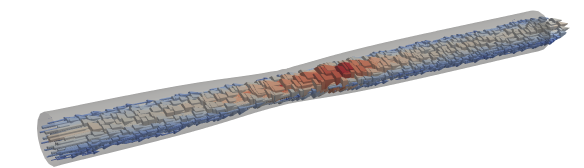


Reconstruction:
We test the methodology with test working domains which are taken different from the geometries in . For each test working domain, we sample target simulations of the governing dynamics in . This yields a total of snapshots per target due to time marching.
We study the performance of our method in terms of relative average reconstruction errors in . For a given target geometry , if we reconstruct by transporting linear subspace from a given template geometry , the relative error for the -th simulation at time is defined as
| (6.3) |
In Figure 5, we fix one target geometry and we show the average error over all simulations , namely
Each curve depicts the error for each template geometry . The role of the routine Best-Template which we have built in the learning stage is to quickly select the template which will be the most appropriate so that we obtain the most accurate reconstruction results. The selection with our proposed construction yields the error curve which is labeled MDS. We tested several possibilities for the definition of the metric but the one based (5.20) produced systematically the best results, so, for the sake of clarity, we only present the results for this choice. We observe in Figure 5 that the selection method is near-optimal in the sense that it chooses either a good or the best available template among the 64 template domains. Figure 6 gives an illustration of the reconstruction of one snapshot with our pipeline.


In addition, it is important to compare with a set of reconstructions on all the test geometries with the pre-computed ROMs . We want to quantify the difference between the PBDW algorithm output of and that of , for . We recall that , and .
It is encouraging to observe that the relative error
is below one percent for a set of 16 ground truth solutions in each test domain , with .
7 Conclusion
We have developed a framework to solve in near-real time state estimation problems for applications that present variations in the spatial domain. For a given target geometry, the reconstruction strategy is based on selecting a relevant linear subspace defined on a template geometry, which is then transported to the target geometry. The reduced model is chosen among a pool of available reduced models, each one defined on a different template geometry. The model selection strategy is based on a dimensionality reduction technique based on MDS. The technique requires defining an appropriate notion of distance between manifold sets from different geometries . Among the different options for the metric which we have tested in our numerical experiments, the one based on formula (5.20) has produced the best results, and is simple to implement in practice. This choice is backed up by our theoretical analysis from Theorem 4.2.
The present contribution paves the way for further developments in the field of inverse problems presenting shape variability, especially in the field of biomedical engineering. Future research will be devoted to applying the present methodology to applications with real data, and with more complex geometrical shapes, with possible time-dependency. In principle, increasing the complexity of the domain can be addressed with the same tools as the ones presented in this paper, which are essentially based on LDDMM (for mappings between surfaces) and MDS (for the search of a Euclidean embedding). However, these techniques will inevitably be increasingly challenged for increasingly complex geometries. For LDDMM, we may require working with more surface points to find a good map between surfaces. In turn, this will challenge the underlying optimization task of LDDMM. As for MDS, it may be necessary to increase the number of available templates geometries to find a good quality embedding, which will increase the computational burden.
Appendix A Details on the numerical solution of the Stokes equation
Using finite elements, we search for the projection coefficients of and in the space of piece-wise linear polynomials and respectively. The Lagrange polynomials are considered on , a tessellation of with tetrahedrons of size cms. We don’t adopt a new notation for the projection of the states in the polynomial spaces when no confusion arises. Time discretization is done via implicit finite differences using a time step of seconds. The semi-discrete weak problem to solve for each reads:
| (A.1) |
, where and are test functions and where denotes the inner product in . In addition, denotes the inner product over a single tetrahedron in . The bilinear form concerning this term is a typical stabilization procedure to deal with the saddle point nature of the problem [53].
The matrix assembly and solution of the monolithic system of equations is done with CPU parallelization via MPI using the software MAD ([54], chapter 5).
Appendix B Numerical implementation of PBDW
This appendix concerns the solution of problem (2.7). We briefly paraphrase and complement the content from [45, Appendix A], where this discussion has been carried out in the context of blood flows.
Let us formulate the problem (2.7) in a discrete framework. We adopt the following definitions and considerations:
- •
Let () be a tessellation of the working domain .
- •
Let be a finite element space on . In the following, we work with a finite element basis for , where is the number of degrees of freedom of any function in .
- •
Let be the mass matrix representing the inner product . For example, in the numerical example of section 6, we have , therefore .
- •
Let be the vector of measurement observations. Each entry is given by .
- •
Let be a matrix where the entry of each column corresponds to the coefficients of the orthonormal Riesz representers on the basis for .
- •
Let be an orthonormal basis for , and a matrix where the entry of each column corresponds to the coefficients of the basis for on the basis for .
- •
Let be the matrix representation of the orthogonal projector . The matrix is given by , where is an identity matrix of size .
In this setting, problem (2.7) can be written in discrete form as follows: We search for a vector , coefficients of on the basis for (i.e. ), reconstruction of , such that:
| (B.1) | ||||
Consider a Lagrange multiplier . The problem can be written without restriction as follows:
| (B.2) | ||||
where the fourth line comes from exploiting the symmetry of and , and the projector property .
Optimality conditions lead to the saddle point problem:
| (B.3) | |||
| (B.4) |
which is a system of equations. Nonetheless, we can reduce the size to with the orthogonal decomposition where
| (B.5) |
In addition, consider the Gramian matrix defined as (of dimensions ) and the expansion of , where . Thus, (B.4) leads to the normal equations
| (B.6) |
Assumption guarantees that the matrix is invertible. Therefore the core operation to solve the original optimization problem (2.7) consists in solving an system of normal equations at online phase to compute , after which it follows that the state is fully computed doing .
The algorithm (and the cost of each step) can be thus summarized as follows:
- •
Offline:
- 1.
Compute the training manifold ( ). depends on the linear solver, tipically .
- 2.
Compute the POD for ().
- 3.
Compute the observation space ().
- 4.
Compute the matrix ().
- 5.
Compute the matrix ().
- 6.
Compute Cholesky factorization ()).
- 1.
- •
Online:
- 1.
Solve the lower-triangular system for by backward substitution ()).
- 2.
Solve the upper-trianguler system for by backward substitution ()).
- 3.
Compute and the solution ().
- 1.
The reader must recall that this is the scheme for the single domain problem (). For the multi domain problem (), the online stage starts from item 3 of offline phase onwards, since the observation space is supposed to be unkown.
References
- [1] D. Amsallem, M. J. Zahr, and C. Farhat. Nonlinear model order reduction based on local reduced-order bases. International Journal for Numerical Methods in Engineering, 92(10):891–916, 2012.
- [2] Gerrit Welper. Interpolation of functions with parameter dependent jumps by transformed snapshots. SIAM Journal on Scientific Computing, 39(4):A1225–A1250, 2017.
- [3] V. Ehrlacher, D. Lombardi, O. Mula, and F.-X. Vialard. Nonlinear model reduction on metric spaces. application to one-dimensional conservative pdes in wasserstein spaces. ESAIM M2AN, 54(6):2159–2197, 2020.
- [4] Bonito A., Cohen A., R. DeVore, D. Guignard, P. Jantsch, and G. Petrova. Nonlinear methods for model reduction. ESAIM: Mathematical Modelling and Numerical Analysis, 55(2):507–531, 2021.
- [5] Y. Maday, A. T. Patera, J. D. Penn, and M. Yano. A parameterized-background data-weak approach to variational data assimilation: formulation, analysis, and application to acoustics. International Journal for Numerical Methods in Engineering, 102(5):933–965, 2015.
- [6] Y. Maday, O. Mula, and G. Turinici. Convergence analysis of the Generalized Empirical Interpolation Method. SIAM Journal on Numerical Analysis, 54(3):1713–1731, 2016.
- [7] P. Binev, A. Cohen, W. Dahmen, R. DeVore, G. Petrova, and P. Wojtaszczyk. Data assimilation in reduced modeling. SIAM/ASA Journal on Uncertainty Quantification, 5(1):1–29, 2017.
- [8] T. Taddei. An adaptive parametrized-background data-weak approach to variational data assimilation. ESAIM: Mathematical Modelling and Numerical Analysis, 51(5):1827–1858, 2017.
- [9] P. Binev, A. Cohen, O. Mula, and J. Nichols. Greedy algorithms for optimal measurements selection in state estimation using reduced models. SIAM/ASA Journal on Uncertainty Quantification, 6(3):1101–1126, 2018.
- [10] H. Gong, Y. Maday, O. Mula, and T. Taddei. PBDW method for state estimation: error analysis for noisy data and nonlinear formulation. arXiv e-prints, page arXiv:1906.00810, Jun 2019.
- [11] A. Cohen, W. Dahmen, R. DeVore, J. Fadili, O. Mula, and J. Nichols. Optimal reduced model algorithms for data-based state estimation. SIAM Journal on Numerical Analysis, 58(6):3355–3381, 2020.
- [12] A. Cohen, W. Dahmen, O. Mula, and J. Nichols. Nonlinear reduced models for state and parameter estimation. arXiv:2009.02687, 2020.
- [13] R. Guibert, K. Mcleod, A. Caiazzo, T. Mansi, M.A. Fernández, M. Sermesant, X. Pennec, I.E. Vignon-Clementel, Y. Boudjemline, and J.F. Gerbeau. Group-wise construction of reduced models for understanding and characterization of pulmonary blood flows from medical images. Medical image analysis, 18(1):63–82, 2014.
- [14] R. Davies, C. Twining, and C. Taylor. Statistical models of shape: Optimisation and evaluation. Springer Science & Business Media, 2008.
- [15] A. Maury, G. Allaire, and F. Jouve. Shape optimisation with the level set method for contact problems in linearised elasticity. The SMAI journal of computational mathematics, 3:249–292, 2017.
- [16] F. De Gournay, G. Allaire, and F. Jouve. Shape and topology optimization of the robust compliance via the level set method. ESAIM: Control, Optimisation and Calculus of Variations, 14(1):43–70, 2008.
- [17] D.L. Colton and R. Kress. Inverse acoustic and electromagnetic scattering theory, volume 93. Springer, 1998.
- [18] F.L. Bookstein. A course in morphometrics for biologists: geometry and statistics for studies of organismal form. Cambridge University Press, 2018.
- [19] P. Mitteroecker and P. Gunz. Advances in geometric morphometrics. Evolutionary Biology, 36(2):235–247, 2009.
- [20] A. E. Løvgren, Y. Maday, and E.M. Rønquist. The reduced basis element method for fluid flows. In Analysis and Simulation of Fluid Dynamics, pages 129–154. Springer, 2006.
- [21] G. Rozza, D.B.P. Huynh, and A. Manzoni. Reduced basis approximation and a posteriori error estimation for Stokes flows in parametrized geometries: roles of the inf-sup stability constants. Numerische Mathematik, 125(1):115–152, 2013.
- [22] A. Manzoni and F. Negri. Efficient reduction of PDEs defined on domains with variable shape. In Model Reduction of Parametrized Systems, pages 183–199. Springer, 2017.
- [23] N. Dal Santo and A. Manzoni. Hyper-reduced order models for parametrized unsteady Navier-Stokes equations on domains with variable shape. Advances in Computational Mathematics, 45(5):2463–2501, 2019.
- [24] L. Chamoin and H.P. Thai. Certified real-time shape optimization using isogeometric analysis, PGD model reduction, and a posteriori error estimation. International Journal for Numerical Methods in Engineering, 119(3):151–176, 2019.
- [25] Fabrizio Garotta, Nicola Demo, Marco Tezzele, Massimo Carraturo, Alessandro Reali, and Gianluigi Rozza. Reduced order isogeometric analysis approach for pdes in parametrized domains. In Quantification of Uncertainty: Improving Efficiency and Technology, pages 153–170. Springer, 2020.
- [26] R. Sevilla, S. Zlotnik, and A. Huerta. Solution of geometrically parametrised problems within a CAD environment via model order reduction. Computer methods in applied mechanics and engineering, 358:112631, 2020.
- [27] L. Piegl and W. Tiller. The NURBS book. Springer Science & Business Media, 1996.
- [28] F. Salmoiraghi, A. Scardigli, H. Telib, and G. Rozza. Free-form deformation, mesh morphing and reduced-order methods: enablers for efficient aerodynamic shape optimisation. International Journal of Computational Fluid Dynamics, 32(4-5):233–247, 2018.
- [29] G. Berkooz, P. Holmes, and J.L. Lumley. The proper orthogonal decomposition in the analysis of turbulent flows. Annual review of fluid mechanics, 25(1):539–575, 1993.
- [30] L. Sirovich. Turbulence and the dynamics of coherent structures. I. coherent structures. Quarterly of applied mathematics, 45(3):561–571, 1987.
- [31] M. Rathinam and L.R. Petzold. A new look at proper orthogonal decomposition. SIAM Journal on Numerical Analysis, 41(5):1893–1925, 2003.
- [32] E.N. Karatzas, G. Stabile, L. Nouveau, G. Scovazzi, and G. Rozza. A reduced basis approach for PDEs on parametrized geometries based on the shifted boundary finite element method and application to a Stokes flow. Computer Methods in Applied Mechanics and Engineering, 347:568–587, 2019.
- [33] N. Akkari, F. Casenave, and D. Ryckelynck. A novel Gappy reduced order method to capture non-parameterized geometrical variation in fluid dynamics problems. 2019.
- [34] E.N. Karatzas, F. Ballarin, and G. Rozza. Projection-based reduced order models for a cut finite element method in parametrized domains. Computers & Mathematics with Applications, 79(3):833–851, 2020.
- [35] G. Stabile, M. Zancanaro, and G. Rozza. Efficient geometrical parametrization for finite-volume-based reduced order methods. International Journal for Numerical Methods in Engineering, 121(12):2655–2682, 2020.
- [36] D. Forti and G. Rozza. Efficient geometrical parametrisation techniques of interfaces for reduced-order modelling: application to fluid–structure interaction coupling problems. International Journal of Computational Fluid Dynamics, 28(3-4):158–169, 2014.
- [37] M.W. Hess and P. Benner. A reduced basis method for microwave semiconductor devices with geometric variations. COMPEL: The International Journal for Computation and Mathematics in Electrical and Electronic Engineering, 2014.
- [38] T. Taddei. A registration method for model order reduction: data compression and geometry reduction. SIAM Journal on Scientific Computing, 42(2):A997–A1027, 2020.
- [39] T. Taddei and L. Zhang. Space-time registration-based model reduction of parameterized one-dimensional hyperbolic PDEs. arXiv preprint arXiv:2004.06693, 2020.
- [40] F. Galarce, J.F. Gerbeau, D. Lombardi, and O. Mula. Fast reconstruction of 3D blood flows from doppler ultrasound images and reduced models. Computer Methods in Applied Mechanics and Engineering, 375:113559, 2021.
- [41] A. Cohen and R. DeVore. Approximation of high-dimensional parametric PDEs. Acta Numerica, 24:1–159, 2015.
- [42] A. Buffa, Y. Maday, A. T. Patera, C. Prud’homme, and G. Turinici. A priori convergence of the greedy algorithm for the parametrized reduced basis method. ESAIM: Mathematical Modelling and Numerical Analysis, 46(3):595–603, 2012.
- [43] G. Rozza, D. B. P. Huynh, and A. T. Patera. Reduced basis approximation and a posteriori error estimation for affinely parametrized elliptic coercive partial differential equations. Archives of Computational Methods in Engineering, 15(3):1, Sep 2007.
- [44] A. Cohen, R. DeVore, and C. Schwab. Analytic regularity and polynomial approximation of parametric and stochastic elliptic PDE’s. Analysis and Applications, 09(01):11–47, 2011.
- [45] F. Galarce, D. Lombardi, and O. Mula. Reconstructing haemodynamics quantities of interest from doppler ultrasound imaging. Int. J. Numer. Meth. Biomedical Eng., 2021.
- [46] Faisal Beg, Michael Miller, Alain Trouvé, and Laurent Younes. Computing large deformation metric mappings via geodesic flows of diffeomorphisms. International Journal of Computer Vision, 65:139–157, 2005.
- [47] H. Murase and S. K. Nayar. Visual learning and recognition of 3D objects from appearance. International journal of computer vision, 14(1):5–24, 1995.
- [48] J. B. Tenenbaum, V. De Silva, and J. C. Langford. A global geometric framework for nonlinear dimensionality reduction. science, 290(5500):2319–2323, 2000.
- [49] D. L. Donoho and C. Grimes. Image manifolds which are isometric to euclidean space. Journal of mathematical imaging and vision, 23(1):5–24, 2005.
- [50] B. Ghojogh, A. Ghodsi, F. Karray, and M. Crowley. Multidimensional scaling, sammon mapping, and isomap: Tutorial and survey. arXiv preprint arXiv:2009.08136, 2020.
- [51] B. Charlier, J. Feydy, J.A. Glaunès, F.D. Collin, and G. Durif. Kernel operations on the GPU, with autodiff, without memory overflows. Journal of Machine Learning Research, 22(74):1–6, 2021.
- [52] P. Ciarlet. Mathematical Elasticity, vol. I, Studies in Mathematics and its Applications, volume 20. North-Holland Publishing Co., 1988.
- [53] F. Brezzi and J. Pitkaranta. On the stabilization of finite element approximations of the Stokes equations. Efficient Solutions of Elliptic Systems, 1984.
- [54] F. Galarce. Inverse problems in hemodynamics. Fast estimation of blood flows from medical data. PhD thesis, INRIA Paris & Laboratoire Jacques-Louis Lions. Sorbonne Université, 2021.