How can we learn (more) from challenges? A statistical approach to driving future algorithm development.
Abstract
Challenges have become the state-of-the-art approach to benchmark image analysis algorithms in a comparative manner. While the validation on identical data sets was a great step forward, results analysis is often restricted to pure ranking tables, leaving relevant questions unanswered. Specifically, little effort has been put into the systematic investigation on what characterizes images in which state-of-the-art algorithms fail. To address this gap in the literature, we (1) present a statistical framework for learning from challenges and (2) instantiate it for the specific task of instrument instance segmentation in laparoscopic videos. Our framework relies on the semantic meta data annotation of images, which serves as foundation for a General Linear Mixed Models (GLMM) analysis. Based on 51,542 meta data annotations performed on 2,728 images, we applied our approach to the results of the Robust Medical Instrument Segmentation Challenge (ROBUST-MIS) challenge 2019 and revealed underexposure, motion and occlusion of instruments as well as the presence of smoke or other objects in the background as major sources of algorithm failure. Our subsequent method development, tailored to the specific remaining issues, yielded a deep learning model with state-of-the-art overall performance and specific strengths in the processing of images in which previous methods tended to fail. Due to the objectivity and generic applicability of our approach, it could become a valuable tool for validation in the field of medical image analysis and beyond. and segmentation of small, crossing, moving and transparent instrument(s) (parts).
1Computer Assisted Medical Interventions (CAMI), German Cancer Research Center (DKFZ), Heidelberg, Germany
2Medical Faculty, Heidelberg University, Heidelberg, Germany
3HIP Helmholtz Imaging Platform, German Cancer Research Center (DKFZ), Heidelberg, Germany
4Department of Mathematics and Computer Science, University of Calabria, Rende, Italy
5Faculty of Mathematics and Computer Science, Heidelberg University, Germany
6Division of Biostatistics, German Cancer Research Center (DKFZ), Heidelberg, Germany
7Section Clinical Tropical Medicine, Heidelberg University, Heidelberg, Germany
8Division of Medical Image Computing (MIC), German Cancer Research Center (DKFZ), Heidelberg, Germany
9The BioRobotics Institute and Department of Excellence in Robotics and AI, Scuola Superiore Sant’Anna, Italy
10Department for General, Visceral and Transplantation Surgery, Heidelberg University Hospital, Heidelberg, Germany
11HIP Applied Computer Vision Lab, MIC, German Cancer Research Center (DKFZ), Heidelberg, Germany
Keywords surgical data science image characteristics driven algorithm development minimally invasive surgery endoscopic vision grand challenges biomedical image analysis challenges generalized linear mixed models instrument segmentation deep learning artificial intelligence
1 Introduction
Comparative performance assessment of image analysis algorithms is typically performed by either reimplementing state-of-the-art methods or by international benchmarking competitions, so-called challenges [1]. As the re-implementation of other methods is prone to errors (e.g., errors in the implementation or suboptimal choice of hyperparameters) and time-consuming, challenges are nowadays the de facto standard for benchmarking new methods.
To date, however, relatively little effort has been put into the systematic analysis of results, as summarized in [2].
Specifically, most reports neglect a particularly relevant question for the medical domain:
What characterizes images on which algorithms fail?
Or, more broadly speaking:
How can we learn from challenge results in a way that enables us to tailor future algorithm development to the specific remaining needs?
Some challenge organizers have recognized this problem and carried out a laborious manual analysis, e.g., by reporting the best and worst cases based on the participants’ performances and identifying a set of image characteristics that could lead to worsening or improving performance (i.e., over-/underexposed images) [3, 4, 5, 6]. However, this approach is rather subjective and does not allow for reliable quantification of the effects of different sources. Furthermore, it may be subject to confirmation bias. Given the lack of systematic analysis methodology, the contribution of this paper is threefold:
- 1.
We present a statistical framework for learning from challenges, which focuses on the identification of sources for algorithm failure (Fig. 1).
- 2.
To demonstrate potential benefit of the new concept, we apply it to the recently published challenge on multi-instance laparoscopic instrument segmentation ROBUST-MIS 11 1 Robust Medical Instrument Segmentation (RobustMIS) Challenge 2019, https://www.synapse.org/#!Synapse:syn18779624/wiki/591266 [3] (see Fig. 2).
- 3.
We demonstrate that knowledge on the identified sources of error can help improve algorithm performance in common failure cases.
Note that this approach was specifically designed for challenges but is similarly applicable to more basic validation studies, in which the performance of only a single algorithm is assessed.

 |
 |
| a) RGB image frame | b) multi-instance segmentation |
The remainder of this paper is structured as follows: After presenting the related work in Sec. 2, we describe our framework for challenge analysis, its application to the task of multi-instance segmentation as well as our strength-weakness-driven algorithm development in Sec. 3. The performed experiments and results are presented in Sec. 4 and discussed in Sec. 5. Sec. 6 concludes this paper by summarizing our main findings.
2 Related Work
In this section, we present the related work on systematic challenge analysis in the field of biomedical image analysis as well as a brief summary on the state of the art in multi-instance medical instrument segmentation.
2.1 Challenge analysis
The literature on the analysis of image analysis challenges is extremely sparse, both within and outside the medical community. In fact, the meta science papers published to date have focused on ranking instabilities [1, 7], standards [8, 1, 9] and challenge visualization [2], while the topic of results analysis has been given extremely little attention. The closest work to ours was only recently published and presents a framework for visualizing challenge results in an uncertainty-aware manner [2]. While sources of error are not addressed within the framework, the paper provided an important motivation for our work: An analysis of numerous challenge reports in the field of biomedical image analysis revealed that a large number (66% of those investigated) report only final ranks or aggregated performance measures [2] without providing further analyses. This finding is in line with our more recent observations: Challenge reports often only provide a website with the rankings (e.g. MISAW22 2 https://www.synapse.org/#!Synapse:syn21776936/wiki/601705, SurgVisDom33 3 https://www.synapse.org/#!Synapse:syn22083820/wiki/606329, EndoVis-WorkFlowChallenge44 4 https://endovissub2017-workflow.grand-challenge.org/PastChallenges/), and corresponding publications concentrate on the presentation of aggregated metric values [10, 11], visual examples [6, 4] or manual inspection of best/worst cases [3]. In fact, we are not aware of any prior work on identifying sources of algorithm failure in a systematic manner.
2.2 Multi-instance segmentation
While the task of binary instrument segmentation received a lot of attention over the last couple of years such as [12, 13, 14, 15, 16], literature on multi-instance segmentation in applications for minimally invasive surgeries is extremely sparse. To our knowledge, the only peer-reviewed work published independently of the ROBUST-MIS challenge [3] (which this work is based on), was published by Shvets et al. [13]. Their work is on robotic instrument segmentation and features a comparatively simplistic data set with respect to image characteristics (e.g., blood, reflections). Hence, the methods competing in the ROBUST-MIS challenge can be regarded as representative for the state of the art in the field.
3 Methods
The following sections present the proposed framework for learning from challenges (Sec. 3.1), its instantiation in the ROBUST-MIS challenge (Sec. 3.2), as well as the proposed deep learning method resulting from problem-tailored algorithm development (Sec. 3.3).
3.1 Framework for learning from challenges
This section introduces our concept for learning from challenges and details the underlying statistical approach.
3.1.1 Concept overview
We propose the following four-step procedure for learning from challenges.
- 1.
Hypothesis generation: In an initial step, potential sources of algorithm failure are identified. These can relate to the image device (e.g. dirty endoscope lens), the imaging protocol (e.g. overexposure/underexposure), the handling of the equipment (e.g. motion blur), the target structure (e.g. crossing medical instruments in the case of ROBUST-MIS) and other application-specific features (e.g. smoke in the field of view of a laparoscope). To generate a list of image characteristics that may lead to poor performance, knowledge from the literature, expert knowledge, personal experience, as well as a manual analysis of the challenge results (as in [3]) can be leveraged.
- 2.
Semantic meta data annotation: (Part of) the challenge test cases are then semantically annotated with these image characteristics. This can be done by domain experts, or by leveraging crowdsourcing, for example.
- 3.
Mixed model analysis: The semantic labels on image characteristics along with the challenge results – represented by (aggregated) metric results per test case – are then leveraged to identify image characteristics leading to poor algorithm performance. To this end, a mixed effects model [17] is set up in which the (possibly transformed) metric values embody the outcome variable and the image-specific information is integrated as explanatory variables. In other words, the performance of an algorithm on a given image is represented as a function of the meta information available for the image. The method is detailed in Sec. 3.1.2.
- 4.
Tailored algorithm development: Based on the identification of those error sources that have the biggest effect on algorithm performance, algorithm development is tailored to the specific problems identified.
Our approach to mixed model-based challenge analysis is detailed in Sec. 3.1.2, followed by an instantiation of this framework in the specific task of multi-instance instrument segmentation in laparoscopic video data in Sec. 3.2.


*Note that metric values may be bounded in theory but appear normally distributed in the specific data set. In this case, no transformation is needed.
**Note that a GLMM for binary outcome is a mixed effect logistic regression model.
3.1.2 Mixed model analysis
As summarized in the previous section, the goal of the statistical analysis is to leverage the semantic meta data annotation to identify image characteristics leading to poor algorithm performance. Standard linear regression models are not suitable for this purpose whenever individual data points are not independent. Non-independence of the data is a typical characteristic of challenges, for example because multiple images from the same patient, or multiple frames from the same video, are used in the analysis. In such a situation, data are best represented by a hierarchical structure. In such a data tree (cf. Fig. 3), data corresponding to the same leaf can be assumed to be independent. Branches represent the source of non-independence, such as a specific hospital, device, or patient. To account for the correlation within challenge outcome data, we propose using Linear Mixed Models (LMMs) [17], as a generalization of linear regression models.
LMMs enable regressing an outcome using a linear combination of explanatory variables weighted by regression coefficients. The outcome variable is also referred to as dependent/target/response/explained variable while the explanatory variables are also called independent variables. In contrast to standard regression models, mixed models not only incorporate the parameters of interest, referred to as fixed effects, but also so-called random effects of variables explaining the hierarchical structure.
In our specific (challenge) setting, image characteristics that have a potential influence on algorithm performance are by default assumed to be binary (present/not present; though categorical variables are also possible) and are represented as fixed effects in the model. Other factors, reflecting the hierarchical structure of the acquired data (e.g. the patient/hospital/image frame identifier) are represented as random effects. The fixed effects coefficients of the model then provide estimates of the impact of the provided image characteristics on the prediction performance. There are several ways to incorporate the challenge participant’s algorithms in this setup. If the specific effects of the (typically small number of) algorithms are of interest, the algorithm can be modeled as a fixed effect, otherwise it is modeled as random effect. Alternatively, as a first approximation, aggregated metric values across algorithms (possibly after transformation; see below) may be used.
Fig. 4 presents a simplified workflow for choosing the appropriate mixed model for a given problem. The specific choice of the mixed model and the process of instantiating depends primarily on the distribution of the metric values. In the case of continuous metric values with unbounded support, an LMM [17] is usually the most natural choice. Applied to the problem of challenge analysis, LMMs can be represented as:
| (1) |
with the following components:
Outcome
The vector represents the metric values on the test images, which may be aggregated over all algorithms or be provided separately for all of them. For clarity of presentation, we will assume a single value per image in the following explanation, but an example of a more fine-grained composition is provided in Sec. 3.2.2.
Fixed effects
The so-called design matrix corresponds to the image characteristics with corresponding fixed effects . Generally, each row of represents an image and consists of binary variables representing the presence or absence of a specific image characteristic on the corresponding image. is the regression coefficient resulting from mixed model fitting, which can be used to predict the dependent variable from the fixed effects. Coefficients are easily interpretable in LMMs with untransformed dependent variables. Given, for example, presence of an image characteristic , the expected metric value changes by compared to the situation when the characteristic is not present. The so-called intercept is a scalar representing an average outcome when all characteristics are absent (the arithmetic mean of ) and is a vector of s.
Random effects
The matrix is a so-called design matrix for the random effects. Assuming, for example, a hierarchical data structure, in which clustering of test images arises from different patients, each patient would represent one of columns in , and each row in the matrix would have exactly one entry with 1 (0 otherwise), reflecting the fact that there is a unique assignment of outcome data to a specific patient. Similarly, further random effects, such as hospital IDs, can be incorporated by increasing the number of columns of (and dimension of ). quantifies the random effect on the specific outcome. For example, the imaging device of a specific hospital could have a lower resolution, hence making predictions more difficult and thus leading to a worse metric value on average. Elements in are assumed to be normally distributed with zero mean and a variance interpreted as the between-cluster-variability (e.g. the variability in performance when comparing images of different hospitals). If the between-cluster-variability is large when compared to the residual variance (see below), observations within the cluster are highly correlated.
Residuals
is a vector of residuals. The residuals are assumed to be normally distributed, capturing the variation in unexplained by the random and fixed effects.
Fitting of the LMM (i.e. estimation of the coefficients) is carried out through restricted maximum likelihood methods (REML). LMMs rely on the assumption of normality of the residuals, i.e., the outcome variable given the values of the explanatory variables follows a normal distribution. To detect a potential violation of the normality constraint, we recommend studying the Q-Q-Plot [18] of the residuals after model fitting. Often, a transformation of the metric values must be applied to obtain approximate normality such that an LMM can be used. For a metric with values , for example, the log transformation is a popular choice; if a metric is bounded by , the logit function, mapping the metric values to , is frequently used. Note that in case of such nonlinear transformation, additivity and linearity of effects on is lost, possibly complicating interpretation of regression coefficients.
If the outcome variable follows a non-normal distribution such as Binomial/Bernoulli, Poisson or Gamma, GLMMs, as a generalization of LMMs can be used ([19]). Specifically, if the outcome variable is binary, a mixed effects logistic regression model as a special case of GLMMs can be used. An instantiation of such a model is provided in Sec. 3.2.2.
3.2 Instantiation of the framework for multi-instance instrument segmentation
As a proof of concept, we instantiated our proposed framework for the ROBUST-MIS challenge 2019 [3]. This challenge was based on 10,040 endoscopic images that had been extracted from three different surgery types [20]. For each test case, the segmentation results of five (one algorithm was excluded due of a non-compliant training process that would affect comparability) participating algorithms were available.
3.2.1 Annotation of image characteristics
To identify potential sources of error, we analyzed the general literature on endoscopic image analysis [21, 22] as well as the specific literature on artifacts in endoscopy [23, 24, 25, 26] and on endoscopic vision challenges [11, 5, 3]). Combined with personal experience gained during the annotation process for the challenge data [20], we identified twelve relevant sources of error (see Table 1) which were classified as global – characterizing the whole image (here: dirty lens, overexposure and underexposure) – or local (e.g. blood on specific instrument instance). The local features were provided for all instrument instances and/or the background individually. A trained engineer with experience in endoscopic image annotation (annotator was part of the annotation team of [20]) then annotated the presence of such characteristics for all images (see Fig. 6). For the relevant test set (stage 3) this resulted in a total of image related and instrument instance annotations.
| LOCAL CHARACTERISTICS | ||
| Characteristic | Bg. | Inst. |
| Covered by blood? | ✓ | ✓ |
| Covered by smoke? | ✓ | ✓ |
| Covered by tissue? | ✗ | ✓ |
| Subject to motion artifacts? | ✓ | ✓ |
| Covered by specular reflections? | ✓ | ✓ |
| Covered by another instrument? | ✗ | ✓ |
| Covered by any other object (non-surgical)? | ✓ | ✓ |
| Too bright? | ✗ | ✓ |
| Too dark? | ✗ | ✓ |
| GLOBAL CHARACTERISTICS | ||
| Characteristic | Img. | |
| Is the image too bright? | ✓ | |
| Is the image too dark? | ✓ | |
| Does the lens seem dirty? | ✓ | |
3.2.2 Statistical analysis
The Dice Similarity Coefficient () [27] is a widely used metric in medical image analysis [1, 7] and also served as a basis for the ranking in the ROBUST-MIS challenge [3]. Yet, as values are in the range of , modeling the algorithm performances directly on the challenge metric would violate the normality assumption of the residuals . As mentioned in Sec. 3.1.2, the problem can potentially be overcome by applying a transformation , such as the logit to metric values bounded in , with the goal of mapping the values to the range of . As this process did not yield an approximate normal residual distribution of for our data, we propose regarding the segmentation problem as a pixel-level classification problem and applying a GLMM to model the target metrics precision and recall as a function of image characteristics, as detailed in the following paragraphs.
Outcome reformulation
For this study, we leverage the fact, that the is closely related to precision () and recall (). More specifically, , and can all be expressed as a function of the number of true(T)/false(F) positives(P)/negatives(N):
| (2) |
| (3) |
To use precision and recall as target metrics, we convert each multi-instance reference annotation mask into a set of binary masks, each corresponding to one instrument instance. For each image , each instrument that is present in and each algorithm we then determine both, the recall, defined as the probability of a pixel of the reference segmentation to be present in the mask provided by the algorithm, and the precision, defined as the probability of a pixel of the segmentation mask to be present in the reference segmentation. In other words, we relate the TP to either the reference mask of an instance (recall) or the mask provided by the algorithm (precision). Formally, the pixel-level classification (per instance) is binary and thus can be regarded as a Bernoulli experiment. Depending on the perspective (recall or precision) if a pixel is correctly classified as instrument follows a Bernoulli distribution with parameter resp. .
GLMM fitting
In GLMMs, a link function relates the expected outcome (here the parameter ) with the linear predictor. The canonical choice for this function in case of binary data is the logit link function . The complete equation is then given by
| (4) |
where is a column-vector consisting of all the probabilities (resp. ) and is applied element-wise. As described above, we define fixed effects for image and instrument characteristics (within ), resulting in . Furthermore, we model the participants’ algorithms, as well as the patient, image and instrument as independent random effects combined in vector (with indicator matrices combined in ), resulting in , where refer to the number of algorithms, the number of patients, the number of images and the total number of instances, respectively. The number of rows in our model comes down to . Note that we inspected the cases of single and multiple instruments per image separately (see Tab. 2). So while and stayed constant there were images with instrument and images with multiple instruments each ( instruments in total).
Model interpretation
After fitting the model, coefficients can be interpreted in terms of log odds ratios (OR) [19]. The OR is a statistic measuring how two events are associated with each other regarding their presence or absence [19]. Here, the OR measures the ratio of the odds (e.g. ) in the presence and absence of a given image characteristic. However, the fact that the OR is not symmetrical around 1 (the value indicating no effect of the image characteristic) makes the comparison of the individual effects less intuitive (as can be illustrated by an OR of 2:3 () and its inverted ratio of 3:2 ()). Fig. 7 thus shows the of the OR, making the values symmetrical around 0. For the interpretation, a positive log OR increases the chance that a high metric is measured, while a negative log OR decreases the chance.
3.3 Strength-weakness-driven algorithm development
As detailed in the results section (Sec. 4.1), the GLMM revealed several image characteristics with major impact on algorithm performance, namely: motion and underexposure of the instrument, crossing medical instruments as well as smoke or other medical equipment (e.g. swabs or bandages) in the field of view. We hypothesized that a majority of these issues can be addressed by going beyond single image analysis and taking the temporal context into account. In fact, the annotators of the Heidelberg Colorectal Data Set for Surgical Data Science in the Sensor Operating Room (HeiCo) [20], which served as basis for the ROBUST-MIS challenge, also reported that analysis of preceding frames was sometimes necessary to label a given frame. The proposed architecture resulting from the GLMM analysis is shown in Fig. 5. The core component of the presented deep learning architecture is a masked region-based convolutional neural network (Mask R-CNN) [28] that uses the following information as input: (1) the raw video frame, (2) the probability of a pixel to be an instrument and (3) the Long short-term memory (LSTM)-summarized information on object motion encoded in an optical flow. Details are provided in A.

4 Experiments and Results
We validated our framework on the ROBUST-MIS challenge 2019 data set [3, 20]. The following sections present our findings with respect to image characteristics impacting algorithm performance as well as the validation of our algorithm tailored to the specific weaknesses of the state of the art.
4.1 Effect of image characteristics on the performance of state-of-the-art algorithms
The frequency of special image characteristics captured by the meta data annotation is shown in Fig. 6.

Following the statistical methodology presented in Sec. 3.2, we analyzed the influence of image characteristics on the algorithm performance, using precision and recall as metrics. The main results are presented in Fig. 7 and Tab. 2.
According to our results, the following main characteristics had a statistically significantly () negative influence on the results: instrument is underexposed, in motion or covered by material, or background is covered by smoke or other objects. Example frames are provided in Fig. 8. When two or more instrument instances were visible (see Fig. 7), the statistically significant characteristic with the largest impact was "instrument covered by another instrument".
| LOCAL CHARACTERISTICS | ||||
| PRECISION | RECALL | |||
| Characteristic | inst. > 1 | inst. = 1 | inst. > 1 | inst. = 1 |
| instrument overexposed | ||||
| instrument covered by tissue | ||||
| instrument underexposed | ||||
| instrument covered by reflections | ||||
| instrument covered by material | ||||
| instrument covered by smoke | ||||
| instrument in motion | ||||
| instrument covered by blood | ||||
| instrument covered by instrument | x | x | ||
| background contains other objects | ||||
| background in motion | ||||
| background covered by blood | ||||
| background covered by reflections | ||||
| background covered by smoke | ||||
| GLOBAL CHARACTERISTICS | ||||
| PRECISION | RECALL | |||
| Characteristic | inst. > 1 | inst. = 1 | inst. > 1 | inst. = 1 |
| image lens dirty | ||||
| image too bright | ||||
| image too dark | ||||

4.2 Performance of algorithm developed based on strength-weakness-analysis
Our method resulting from the strength-weakness-analysis was compared to the ROBUST-MIS 2019 challenge’s top-scoring methods based on the accuracy as reported in the ROBUST-MIS challenge [3] and using the challengeR analysis tool [2]. For the validation of our method, we used the metrics proposed by the ROBUST-MIS challenge as this allowed us to compare it to the best-performing related methods. Following the challenge guidelines [3], we split the data into 5,983 training and 4,057 test images. The reason for the relatively high number of test images compared to training images was the fact that we reserved one surgery type exclusively for testing, as detailed in [3]. As shown in Fig. 10, our method outperformed the state of the art in the majority of categories that represent typical failure cases.
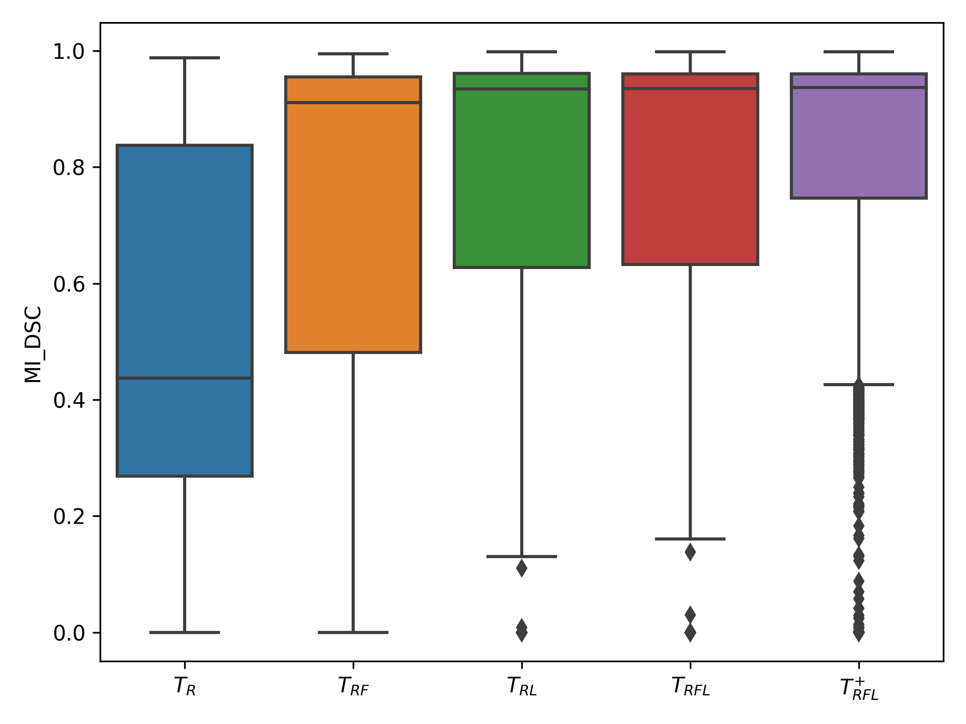
We further performed an ablation study to assess the benefit of the different architectures components, namely (1) the optical flow and (2) the instrument likelihood as additional input to the Mask R-CNN and (3) our post-processing method applied to the output of the Mask R-CNN. The results are presented in Fig. 9. Including the optical flow ( vs. ) improved the performance by a factor of , from a median MI_DSC of to (mean: to ()). Including the instrument likelihood in the network model () also increased the median MI_DSC by a factor of ( to (); mean to ()). Incorporating both the flow and the instrument likelihood as additional input () did not yield a substantial improvement compared to .
The post-processing significantly () increases the mean performance of the model at , while simultaneously reducing the IQR from to . Also, the robustness of the method (defined in [3] as the 5th percentile) increased from to . Further descriptive statistics can be found in Tab. 3.
| Model | |||||||
|---|---|---|---|---|---|---|---|
| 0.50 | 0.44 | 0.00 | 0.27 | 0.83 | 0.56 | ||
| 0.73 | 0.91 | 0.0 | 0.48 | 0.95 | 0.47 | ||
| 0.79 | 0.93 | 0.24 | 0.63 | 0.96 | 0.33 | ||
| 0.80 | 0.93 | 0.29 | 0.63 | 0.96 | 0.33 | ||
| 0.80 | 0.93 | 0.29 | 0.63 | 0.96 | 0.33 | ||
| 0.81 | 0.94 | 0.32 | 0.75 | 0.96 | 0.21 |

5 Discussion
While a lot of research is currently invested in maximizing algorithm performance for various image analysis tasks, comparatively little effort is currently put into failure analysis. This holds especially true for the growing field of benchmarking via challenges. Although challenge results potentially encode crucial information with respect to typical failure cases as well as reasons for algorithm failure, most challenge organizers restrict their reports to plain ranking tables [2] leaving the rich challenge data unexploited. To address this gap in the literature, we presented a statistical framework for systematically learning from challenge results and instantiated it for the specific task of medical instrument segmentation. The following sections discuss the general approach (Sec. 5.1), the specific findings for the sample application (Sec. 5.2) as well the new algorithm resulting from the statistical analysis (Sec. 5.3).
5.1 Framework for challenge analysis
In the field of biomedical image processing, failure analysis is often restricted to qualitative assessments [2]. Even quantitative analyses are typically restricted to single parameter assessments contrasting algorithm performance in the presence or absence of certain features (e.g. [26]). This approach should be used cautiously as it neglects a possible strong interplay between features, thus potentially confusing correlation with causation. We overcome these limitations by a statistically well-grounded approach. Leveraging the strengths of mixed models, we are able to disentangle the effects of different sources and clearly identify sources of algorithm failure. This enables the design of future algorithms dedicated to the actual needs.
A limitation of our concept is the additional manual annotation effort involved. Depending on the specific application, this could potentially be overcome by an automatic annotation of image characteristics, or by (quality-controlled) crowdsourcing [30, 31]. It should further be noted that we instantiated the concept only for a single challenge, with specific focus on multi-instance medical instrument segmentation. However, as segmentation is by far the most widely used task in challenges [1], our concept can be transferred to a majority of studies and also create awareness of the problem that arises when using statistical tests for bounded metrics. Finally, it must be noted that statistical modelling is a complex process of balancing adherence to specific assumptions and model complexity. Delivering a recipe applicable to every challenge is not possible within the scope of a single paper but we believe that this work could trigger more sophisticated challenge analyses following the general approach presented here.
5.2 Instantiation for ROBUST-MIS challenge
In contrast to the literature (e.g., [21, 22, 23, 24, 25, 26, 11, 5, 3]), our study did not reveal a harmful effect of reflections, blood, and smoke on the algorithm performances. Instead, our analysis showed that the main limiting factors are when an instrument is in motion, underexposed, or covered by another instrument. Interestingly, other characteristics such as an instrument being overexposed or covered by tissue, reflections or blood, seem to even support the algorithm performances. That artifacts/characteristics are not always harmful is in line with a recent work from [32] who use reflections to improve the segmentation of polyps. The fact that the characteristic "instrument covered by tissue" has a slight positive effect on algorithm performence is most likely due to the fact that the visible tissue overlay mainly occurs when the instrument is clearly visible and distinguishable from the background.
While most of the characteristics either harm or benefit both metrics investigated, we identified one characteristic that yielded different results for precision and recall. Specifically, when the background contains other objects, we observe an increased recall but a decreased precision. This indicates that an oversegmentation occurred typically occurred in these cases.
The strongest negative impact by far was found when the instrument is being covered by another instrument. This can be attributed to the architecture of Mask R-CNNs and their way of processing images. A Mask R-CNN relies on a region proposal network that provides bounding boxes around regions of particular interest. Especially in regions where instruments overlap, those bounding boxes might contain parts of multiple instrument instances, which then leads to poor segmentations. This finding is in line with work on the Mask R-CNN problem of overlapping instances [33].
5.3 Algorithm development tailored to failure cases
With a few exceptions [34, 35]), the few methods published on multi-instance segmentation to date use a Mask R-CNN [36, 37] as core component. To our knowledge, Kletz et al. [37] were the first to use a Mask R-CNN for surgical instrument segmentation. They developed their method for laparoscopic gynecology videos but reported limitations under conditions of occlusion and overlapping instruments. In the context of binary segmentation, several authors have aimed to tackle this issue by including temporal information in order to improve their segmentation, e.g., in situations where instruments are only partially visible, due to overlapping tissue. Jin et al. [14] were the first who estimated the optical flow by using a CNN, namely UnFlow [38], for the segmentation of instruments. Instead of using the optical flow as an additional feature, they used it as a prior for initializing the attention of a temporal attention pyramid network to learn to focus on moving objects. However, their approach was for binary segmentation, type classification and instrument parts segmentation and classification, thus requiring a much simpler network architecture and no management of pixels that could possibly belong to different object instances.
The first to combine a Mask R-CNN and the optical flow were González et al. [36], who proposed the use of a Mask-RCNN to ensure a segmentation and classification of instruments as, e.g., grasper or scissors. The authors computed the optical flow of previous frames to include a temporal consistency module and consider an instance’s predictions across the frames in a sequence. The approach outperformed the state-of-the-art methods on the Endoscopic Vision 2017 and 2018 Robotic Instrument Segmentation data sets [6]. However, this work was also not used for multi-instance segmentation.
Up to this point, and to the best of our knowledge, none of the approaches for multi-instance segmentation have successfully incorporated temporal information in the algorithm, as further reported by [3]. To address this gap in the literature, a new algorithm was developed that generated a benefit using optical flow in combination with instrument probability in order to explicitly address the previously mentioned weaknesses. While we found a huge performance boost when integrating the flow as an additional input of a native Mask R-CNN, the effect was negligible when also incorporating instrument likelikehood. In contrast, we achieved a high performance boost with an additional post-processing step dedicated to resolving ambiguities in the presence of overlapping instruments.
The presented results suggest that typical challenges of laparoscopic videos, such as reflection, blood, and lighting variations, are already well manageable by state-of-the-art methods. However, difficulties with tube-like structures that are misclassified as instruments or transparent objects such as trocars persist. Furthermore, images with crossing or close instruments remain difficult to separate for both state-of-the-art methods and the presented approach, even though the latter was specially designed to manage such difficulties. One limiting factor may be seen in restrictions in the training and test data set, where only 8% of the images contain more than two instrument instances. Furthermore, only in rare cases do those instances overlap or intersect, thus resulting in only limited opportunities for training and evaluating the algorithm’s separation capabilities.
It should be mentioned that real-time capability is an essential prerequisite for successful translation to a clinical setting. Currently, the Conditional Random Field (CRF) A.4 and the estimation of the optical flow would already approximately take more than 2 seconds per image. However, the method presented was merely an attempt to solve the multi-instance segmentation problem. The next step could be rendering the algorithm real-time capable.
Overall, our methodology achieved a new best score on the ROBUST-MIS challenge data set. While we did not use the challenge test data to tune hyperparameters, it should be mentioned that we had access to the other participants’ performance results to inform the strength-weakness driven algorithm development. This could still be seen as a competitive advantage. However, the primary aim of this study was not to present a new state-of-the-art method for instrument segmentation but a novel concept for learning from challenges. With this work, we have not only identified typical failure cases for the task of medical instrument segmentation but also showcased an entirely new way of problem-driven algorithm development based on insights gained through challenge results.
6 Conclusion
In conclusion, the proposed approach to leveraging meta data annotations for a mixed model-based analysis of challenge results opens up entirely new opportunities for systematically learning from challenges. By identification of characteristics that lead to algorithm failure it not only provides a much deeper understanding of the state of the art for a given application but also enables tailoring future algorithm development to the actual remaining needs.
Acknowledgments and conflicts of interest
The authors would like to thank Minu Dietlinde Tizabi and Alexander Seitel for proofreading the paper. Part of this work was funded by the Helmholtz Imaging Platform (HIP), a platform of the Helmholtz Incubator on Information and Data Science and by the Surgical Oncology Program of the National Center for Tumor Diseases (NCT) Heidelberg. Finally, thanks to all authors of the ROBUST-MIS challenge manuscript [39], which served as foundation of this work.
References
- [1] Lena Maier-Hein, Matthias Eisenmann, Annika Reinke, Sinan Onogur, Marko Stankovic, Patrick Scholz, Tal Arbel, Hrvoje Bogunovic, Andrew P Bradley, Aaron Carass, et al. Why rankings of biomedical image analysis competitions should be interpreted with care. Nature communications, 9(1):5217, 2018.
- [2] Manuel Wiesenfarth, Annika Reinke, Bennett A Landman, Matthias Eisenmann, Laura Aguilera Saiz, M Jorge Cardoso, Lena Maier-Hein, and Annette Kopp-Schneider. Methods and open-source toolkit for analyzing and visualizing challenge results. Scientific Reports, 11(1):1–15, 2021.
- [3] Tobias Roß, Annika Reinke, Peter M. Full, Martin Wagner, Hannes Kenngott, Martin Apitz, Hellena Hempe, Diana Mindroc Filimon, Patrick Scholz, Thuy Nuong Tran, Pierangela Bruno, Pablo Arbeláez, Gui-Bin Bian, Sebastian Bodenstedt, Jon Lindström Bolmgren, Laura Bravo-Sánchez, Hua-Bin Chen, Cristina González, Dong Guo, Pål Halvorsen, Pheng-Ann Heng, Enes Hosgor, Zeng-Guang Hou, Fabian Isensee, Debesh Jha, Tingting Jiang, Yueming Jin, Kadir Kirtac, Sabrina Kletz, Stefan Leger, Zhixuan Li, Klaus H. Maier-Hein, Zhen-Liang Ni, Michael A. Riegler, Klaus Schoeffmann, Ruohua Shi, Stefanie Speidel, Michael Stenzel, Isabell Twick, Gutai Wang, Jiacheng Wang, Liansheng Wang, Lu Wang, Yujie Zhang, Yan-Jie Zhou, Lei Zhu, Manuel Wiesenfarth, Annette Kopp-Schneider, Beat P. Müller-Stich, and Lena Maier-Hein. Comparative validation of multi-instance instrument segmentation in endoscopy: results of the robust-mis 2019 challenge. Medical Image Analysis, page 101920, 2020.
- [4] Max Allan, Jonathan Mcleod, Cong Cong Wang, Jean Claude Rosenthal, Ke Xue Fu, Trevor Zeffiro, Wenyao Xia, Zhu Zhanshi, Huoling Luo, Xiran Zhang, et al. Stereo correspondence and reconstruction of endoscopic data challenge. arXiv preprint arXiv:2101.01133, 2021.
- [5] Max Allan, Satoshi Kondo, Sebastian Bodenstedt, Stefan Leger, Rahim Kadkhodamohammadi, Imanol Luengo, Felix Fuentes, Evangello Flouty, Ahmed Mohammed, Marius Pedersen, et al. 2018 robotic scene segmentation challenge. arXiv preprint arXiv:2001.11190, 2020.
- [6] Max Allan, Alex Shvets, Thomas Kurmann, Zichen Zhang, Rahul Duggal, Yun-Hsuan Su, Nicola Rieke, Iro Laina, Niveditha Kalavakonda, Sebastian Bodenstedt, et al. 2017 robotic instrument segmentation challenge. Available online at: arXiv preprint arXiv:1902.06426, 2019.
- [7] Annika Reinke, Matthias Eisenmann, Sinan Onogur, Marko Stankovic, Patrick Scholz, Peter M Full, Hrvoje Bogunovic, Bennett A Landman, Oskar Maier, Bjoern Menze, et al. How to exploit weaknesses in biomedical challenge design and organization. In International Conference on Medical Image Computing and Computer-Assisted Intervention, pages 388–395. Springer, 2018.
- [8] Adriënne M Mendrik and Stephen R Aylward. A framework for challenge design: Insight and deployment challenges to address medical image analysis problems. arXiv preprint arXiv:1911.08531, 2019.
- [9] Lena Maier-Hein, Annika Reinke, Michal Kozubek, Anne L Martel, Tal Arbel, Matthias Eisenmann, Allan Hanbury, Pierre Jannin, Henning Müller, Sinan Onogur, et al. Bias: Transparent reporting of biomedical image analysis challenges. Medical image analysis, 66:101796, 2020.
- [10] Hassan Al Hajj, Mathieu Lamard, Pierre-Henri Conze, Soumali Roychowdhury, Xiaowei Hu, Gabija Maršalkaitė, Odysseas Zisimopoulos, Muneer Ahmad Dedmari, Fenqiang Zhao, Jonas Prellberg, et al. Cataracts: Challenge on automatic tool annotation for cataract surgery. Medical image analysis, 52:24–41, 2019.
- [11] Sebastian Bodenstedt, Max Allan, Anthony Agustinos, Xiaofei Du, Luis Garcia-Peraza-Herrera, Hannes Kenngott, Thomas Kurmann, Beat Müller-Stich, Sebastien Ourselin, Daniil Pakhomov, et al. Comparative evaluation of instrument segmentation and tracking methods in minimally invasive surgery. arXiv preprint arXiv:1805.02475, 2018.
- [12] Eung-Joo Lee, William Plishker, Xinyang Liu, Timothy Kane, Shuvra S Bhattacharyya, and Raj Shekhar. Segmentation of surgical instruments in laparoscopic videos: training dataset generation and deep-learning-based framework. In Medical Imaging 2019: Image-Guided Procedures, Robotic Interventions, and Modeling, volume 10951, page 109511T. International Society for Optics and Photonics, 2019.
- [13] Alexey A Shvets, Alexander Rakhlin, Alexandr A Kalinin, and Vladimir I Iglovikov. Automatic instrument segmentation in robot-assisted surgery using deep learning. In IEEE International Conference on Machine Learning and Applications), pages 624–628. IEEE, 2018.
- [14] Yueming Jin, Keyun Cheng, Qi Dou, and Pheng-Ann Heng. Incorporating temporal prior from motion flow for instrument segmentation in minimally invasive surgery video. In International Conference on Medical Image Computing and Computer-Assisted Intervention, pages 440–448. Springer, 2019.
- [15] Max Allan, Ping-Lin Chang, Sébastien Ourselin, David J Hawkes, Ashwin Sridhar, John Kelly, and Danail Stoyanov. Image based surgical instrument pose estimation with multi-class labelling and optical flow. In International Conference on Medical Image Computing and Computer-Assisted Intervention, pages 331–338. Springer, 2015.
- [16] Luis C García-Peraza-Herrera, Wenqi Li, Caspar Gruijthuijsen, Alain Devreker, George Attilakos, Jan Deprest, Emmanuel Vander Poorten, Danail Stoyanov, Tom Vercauteren, and Sébastien Ourselin. Real-time segmentation of non-rigid surgical tools based on deep learning and tracking. In International Workshop on Computer-Assisted and Robotic Endoscopy, pages 84–95. Springer, 2016.
- [17] Brady T West, Kathleen B Welch, and Andrzej T Galecki. Linear mixed models: a practical guide using statistical software. Crc Press, 2014.
- [18] Henry C Thode. Testing for normality, volume 164. CRC press, 2002.
- [19] C.E. McCulloch, S.R. Searle, and J.M. Neuhaus. Generalized, Linear, and Mixed Models. Wiley Series in Probability and Statistics. Wiley, 2011.
- [20] Lena Maier-Hein, Martin Wagner, Tobias Ross, Annika Reinke, Sebastian Bodenstedt, Peter M. Full, Hellena Hempe, Diana Mindroc-Filimon, Patrick Scholz, Thuy Nuong Tran, Pierangela Bruno, Anna Kisilenko, Benjamin Müller, Tornike Davitashvili, Manuela Capek, Minu D. Tizabi, Matthias Eisenmann, Tim J. Adler, Janek Gröhl, Melanie Schellenberg, Silvia Seidlitz, T. Y. Emmy Lai, Bünyamin Pekdemir, Veith Roethlingshoefer, Fabian Both, Sebastian Bittel, Marc Mengler, Lars Mündermann, Martin Apitz, Annette Kopp-Schneider, Stefanie Speidel, Felix Nickel, Pascal Probst, Hannes G. Kenngott, and Beat P. Müller-Stich. Heidelberg colorectal data set for surgical data science in the sensor operating room. Scientific Data, 8(1):101, Apr 2021.
- [21] Lena Maier-Hein, Anja Groch, Adrien Bartoli, Sebastian Bodenstedt, G Boissonnat, P-L Chang, NT Clancy, Daniel S Elson, Sven Haase, Eric Heim, et al. Comparative validation of single-shot optical techniques for laparoscopic 3-d surface reconstruction. IEEE transactions on medical imaging, 33(10):1913–1930, 2014.
- [22] Sharib Ali, Felix Zhou, Adam Bailey, Barbara Braden, James E East, Xin Lu, and Jens Rittscher. A deep learning framework for quality assessment and restoration in video endoscopy. Medical Image Analysis, 68:101900, 2021.
- [23] Sharib Ali, Felix Zhou, Barbara Braden, Adam Bailey, Suhui Yang, Guanju Cheng, Pengyi Zhang, Xiaoqiong Li, Maxime Kayser, Roger D Soberanis-Mukul, et al. An objective comparison of detection and segmentation algorithms for artefacts in clinical endoscopy. Scientific reports, 10(1):1–15, 2020.
- [24] Sharib Ali, Mariia Dmitrieva, Noha Ghatwary, Sophia Bano, Gorkem Polat, Alptekin Temizel, Adrian Krenzer, Amar Hekalo, Yun Bo Guo, Bogdan Matuszewski, et al. Deep learning for detection and segmentation of artefact and disease instances in gastrointestinal endoscopy. Medical Image Analysis, page 102002, 2021.
- [25] Isabel Funke, Sebastian Bodenstedt, Carina Riediger, Jürgen Weitz, and Stefanie Speidel. Generative adversarial networks for specular highlight removal in endoscopic images. In Medical Imaging 2018: Image-Guided Procedures, Robotic Interventions, and Modeling, volume 10576, page 1057604. International Society for Optics and Photonics, 2018.
- [26] Roger D Soberanis-Mukul, Shadi Albarqouni, and Nassir Navab. Polyp-artifact relationship analysis using graph inductive learned representations. arXiv preprint arXiv:2009.07109, 2020.
- [27] Lee R Dice. Measures of the amount of ecologic association between species. Ecology, 26(3):297–302, 1945.
- [28] Kaiming He, Georgia Gkioxari, Piotr Dollár, and Ross Girshick. Mask R-CNN. In IEEE International Conference on Computer Vision, pages 2961–2969, 2017.
- [29] Eddy Ilg, Nikolaus Mayer, Tonmoy Saikia, Margret Keuper, Alexey Dosovitskiy, and Thomas Brox. FlowNet 2.0: Evolution of optical flow estimation with deep networks. pages 2462–2470, 2017.
- [30] Lena Maier-Hein, Sven Mersmann, Daniel Kondermann, Christian Stock, Hannes Gotz Kenngott, Alexandro Sanchez, Martin Wagner, Anas Preukschas, Anna-Laura Wekerle, Stefanie Helfert, et al. Crowdsourcing for reference correspondence generation in endoscopic images. In International conference on medical image computing and computer-assisted intervention, pages 349–356. Springer, 2014.
- [31] Eric Heim, Tobias Roß, Alexander Seitel, Keno März, Bram Stieltjes, Matthias Eisenmann, Johannes Lebert, Jasmin Metzger, Gregor Sommer, Alexander W Sauter, et al. Large-scale medical image annotation with crowd-powered algorithms. Journal of Medical Imaging, 5(3):034002, 2018.
- [32] Maxime Kayser, Roger D Soberanis-Mukul, Anna-Maria Zvereva, Peter Klare, Nassir Navab, and Shadi Albarqouni. Understanding the effects of artifacts on automated polyp detection and incorporating that knowledge via learning without forgetting. arXiv preprint arXiv:2002.02883, 2020.
- [33] Shichao Xu, Shuyue Lan, and Zhu Qi. Maskplus: Improving mask generation for instance segmentation. In Proceedings of the IEEE/CVF Winter Conference on Applications of Computer Vision, pages 2030–2038, 2020.
- [34] SM Kamrul Hasan and Cristian A Linte. U-netplus: A modified encoder-decoder u-net architecture for semantic and instance segmentation of surgical instruments from laparoscopic images. In 2019 41st Annual International Conference of the IEEE Engineering in Medicine and Biology Society (EMBC), pages 7205–7211. IEEE, 2019.
- [35] Fabian Isensee and Klaus H Maier-Hein. Or-unet: an optimized robust residual u-net for instrument segmentation in endoscopic images. arXiv preprint arXiv:2004.12668, 2020.
- [36] Cristina González, Laura Bravo-Sánchez, and Pablo Arbelaez. Isinet: An instance-based approach for surgical instrument segmentation. In International Conference on Medical Image Computing and Computer-Assisted Intervention, pages 595–605. Springer, 2020.
- [37] Sabrina Kletz, Klaus Schoeffmann, Jenny Benois-Pineau, and Heinrich Husslein. Identifying surgical instruments in laparoscopy using deep learning instance segmentation. In IEEE International Conference on Content-Based Multimedia Indexing, pages 1–6. IEEE, 2019.
- [38] Simon Meister, Junhwa Hur, and Stefan Roth. Unflow: Unsupervised learning of optical flow with a bidirectional census loss. In Thirty-Second AAAI Conference on Artificial Intelligence, 2018.
- [39] Tobias Roß, Annika Reinke, and Lena Maier-Hein. Robust medical instrument segmentation (ROBUST-MIS) challenge (grand-challenge.org), 2019. https://robustmis2019.grand-challenge.org/. Accessed: 2019-10-29.
- [40] Olaf Ronneberger, Philipp Fischer, and Thomas Brox. U-net: Convolutional networks for biomedical image segmentation. In International Conference on Medical Image Computing and Computer-Assisted Intervention, pages 234–241. Springer, 2015.
- [41] Javier Sánchez, Agustín Salgado, and Nelson Monzón. Computing inverse optical flow. Pattern Recognition Letters, 52:32–39, 2015.
- [42] Sepp Hochreiter and Jürgen Schmidhuber. Long short-term memory. Neural computation, 9(8):1735–1780, 1997.
- [43] Paul Jaccard. The distribution of the flora in the alpine zone. 1. New phytologist, 11(2):37–50, 1912.
- [44] Maria Robu, Abdolrahim Kadkhodamohammadi, Imanol Luengo, and Danail Stoyanov. Towards real-time multiple surgical tool tracking. Computer Methods in Biomechanics and Biomedical Engineering: Imaging & Visualization, pages 1–7, 2020.
- [45] John Lafferty, Andrew McCallum, and Fernando CN Pereira. Conditional random fields: Probabilistic models for segmenting and labeling sequence data. 2001.
- [46] Linda G Shapiro. Connected component labeling and adjacency graph construction. In Machine Intelligence and Pattern Recognition, volume 19, pages 1–30. Elsevier, 1996.
- [47] Jack Kiefer, Jacob Wolfowitz, et al. Stochastic estimation of the maximum of a regression function. The Annals of Mathematical Statistics, 23(3):462–466, 1952.
Appendix
Appendix A Segmentation algorithm
Formally, the multi-instance instrument segmentation problem is defined as follows: Given is a video sequence that consists of frames. All frames have the dimensions , where and are the image height and width, and the three channels in the last dimension contain the RGB-encoded color information. To the final frame of corresponds a set of instrument instances present in frame , that have to be segmented.
Our basic approach was briefly presented in Sec. 3.3 and illustrated in our overview Fig. 5. The following sections present the details of the instrument likelihood prediction in Sec. A.1, the method for flow estimation in Sec. A.2, the final prediction of instrument instances in Sec. A.3 and the post-processing in Sec. A.4.
A.1 Instrument likelihood prediction
Given a video sequence , the goal of this step is to predict within the final frame of for each pixel in the probability that it is an instrument. Arranged as the original image shape this yields the likelihood map as output of the binary segmentation model . Prediction is done with a 2D U-Net [40], which achieved the best results in the ROBUST-MIS binary segmentation challenge [3] and is further described in Isensee et al. [35].
A.2 Usage of the temporal information
For segmenting instrument instances in the final frame of a video sequence , the goal is to include the knowledge of the previous frames . In the first step, the instrument motion is estimated using the optical flow concept. In the second step, this movement is summarized so as to enable straightforward processing in the segmentation task. The following two paragraphs will explain how the optical flow is generated and summarized for later use in the segmentation network.
Prediction of the optical flow
Prediction of the optical flow is done for two consecutive frames and at a given time step via FlowNet2 [29] , such that . The dimensions of are . The two layers in the last dimension correspond to the shift of each pixel in x- (first layer) and y- (second layer) direction. Estimation of the optical flow is defined to be backwards in time, from , to . Defining this is important because the optical flow estimation is not symmetric due to effects such as occluded regions [41].
Summarizing the optical flow
To summarize the optical flow as a latent representation of the motion in the complete sequence of length , as model , a recurrent neural network in the form of a LSTM was chosen [42]. We decided to summarize the optical flow separately, but with the same network, in the x- and y- direction, which led to the latent representation with the dimensions :
| (5) |
A.3 Segmentation of multiple instances
Recall, we are given a video sequence of length , where for the last video frame , all instrument instances that are present in should be segmented. As the number of visible instances differs from image to image, a Mask R-CNN was used as a segmentation model . To keep the same spatial dimensions, the input of is the concatenation in the last dimension of the RGB image , the likelihood of a pixel being an instrument and the latent space of the motion over all video frames :
| (6) |
where is a set of predictions that yields pairs of predicted instances with its corresponding predicted Intersection over Union () score [43] and being the number of predicted instances. The dimensions of a are , with values within that are the probabilities of the image pixels belonging to instance number , while is a value within .
Since the Mask R-CNN often produces thousands of candidates in an image, only instances that have a high predicted of the bounding box above a threshold are considered as valid instances. After thresholding, each pixel is usually assigned to an instance number by performing the per pixel to obtain the highest probability for an instance number. However, this procedure might lead to problems, as will be explained in the next paragraph.
A.4 Post-processing
One of the peculiarities in the endoscopic instrument segmentation occurs in cases where instruments overlap or are only partially visible on the side of an image. In both cases the bounding box proposals may overlap, with all containing a high score which can make it difficult to proceed. These bounding box ambiguities [44] can, when the usual pixel-wise operation is performed on the results, lead to a segmentation with mixed and distributed instance numbers.
Remove overlapping instances
As usual, when working with Mask R-CNN, during the first step all predicted instances that have a score greater than are considered as valid instances . In the second step, however, all valid instances are pairwise compared with the metric to find proposals that have a large overlap (where denotes the number of pixels in the instance ). In every case, where the instances have a high degree of overlap (), the proposal with fewer pixels is removed.
Refine labels
After multiple proposals for the same instance were removed, there remains the possibility of overlapping bounding boxes, especially in the case where instruments overlap (see Fig. 11).

|

|
| a) Image with bounding box proposals | b) Segmentation before post-processing |
 | |
| c) Segmentation after post-processing | |
For this purpose, a Conditional Random Field [45] is used, where the unary energy is defined as the probability of each pixel belonging to an instance. After fitting the CRF, the operation is applied on each pixel to assign the corresponding instrument instance number. In a final check, the result of the is binarized and compared to the binary segmentation from the instrument likelihood prediction. If only small regions of pixels are left (number of pixels ), a connected component analysis [46] is performed to assign those small regions to the labels previously assigned with the CRF. If there are still large areas of instruments remaining, those are added as an additional class to the CRF and the CRF is fitted again to include the missing pixels. The results of the post-processing can be seen in Fig. 11
A.5 Implementation details
All parameters were set according to small experiments on a held-out validation set during the implementation process.
Instrument likelihood prediction
The instrument likelihood prediction is based on the semantic instrument segmentation method of Isensee et al. [35] and thus uses an ensemble vote of eight models that were trained by omitting one surgery on an 8-fold cross-validation. Each model was trained for epochs using randomly selected patches at a size of , where an epoch was defined as an iteration of over 100 batches. To prevent overfitting, the following data augmentation techniques were randomly applied on each image during training: contrast, brightness and gamma-augmentation, image rotation, scaling, mirroring, elastic deformation and additive Gaussian noise [35]. The optimizer was the SGD [47], with an initial learning rate of which decayed to over the course of the training [35].
The prediction model was trained with the following loss , a combination of the regular pixel-wise cross-entropy loss (Eq. 7) and the soft dice loss (Eq. 8).
| (7) |
| (8) |
Where is the reference value and is the estimated probability value for a given pixel , are soft true positives, are soft false negatives and are soft false positives).
Image flow prediction
For all experiments, the optical flow was computed via a video sequence that lasted . Since using the original video frame rate of fps would result in a vanishing gradient and require too much memory, the optical flow was computed with lowered frame rate of only fps. This resulted in an optical flow with the resolution of . As the computation of the optical flow is resource-intensive, it was pre-computed and stored.
Summarized was the optical flow with the LSTM using hidden convolutional layers of dimension . The optical flow consists of two components (x / y component), each being summarized on its own, but all components with the same model.
A.6 Multi-instance segmentation
The Mask R-CNN is based on a ResNet-50 backbone, with the anchor sizes of and aspect ratios of . The detection threshold was in order to also detect small instrument boundaries. For training the model, the SGD optimizer was used, with a momentum of , a learning rate of and a batch consisting of samples. To prevent the training from crashing, all gradients were clipped at . Since the meaning of the optical flow is not invariant to augmentation techniques that change pixel locations, no data augmentation techniques were used. Only the image dimension was halved, with respect to the optical flow vector.
A.7 Post-processing
For the post-processing, (overlap between proposals) was set to and (very small pixel regions) was set to . The parameters were estimated on a small validation set that was randomly taken from the training data set.