Market Complete Option Valuation using a Jarrow-Rudd Pricing Tree with Skewness and Kurtosis

Yuan Hu Affiliation: Department of Mathematics & Statistics, Texas Tech University, Lubbock, TX 79409-1042, USA
yuan.hu@ttu.edu; abootaleb.shirvani@ttu.edu; zari.rachev@ttu.edu Abootaleb Shirvani Affiliation: Department of Mathematics & Statistics, Texas Tech University, Lubbock, TX 79409-1042, USA
yuan.hu@ttu.edu; abootaleb.shirvani@ttu.edu; zari.rachev@ttu.edu Affiliation: Present address: Department of Actuarial Science & Risk Management, Drake University, Des Moines, IA, 50311, USA W. Brent Lindquist Affiliation: Department of Mathematics & Statistics, Texas Tech University, Lubbock, TX 79409-1042, USA
yuan.hu@ttu.edu; abootaleb.shirvani@ttu.edu; zari.rachev@ttu.edu Affiliation: Corresponding author: brent.lindquist@ttu.edu Frank J. Fabozzi Affiliation: Finance Department, EDHEC Business School, 393/400 Promenade des Anglais-BP3116, CEDEX 3, 06202 Nice, France
frank.fabozzi@edhec.edu Svetlozar T. Rachev Affiliation: Department of Mathematics & Statistics, Texas Tech University, Lubbock, TX 79409-1042, USA
yuan.hu@ttu.edu; abootaleb.shirvani@ttu.edu; zari.rachev@ttu.edu

Abstract Applying the Cherny-Shiryaev-Yor invariance principle, we introduce a generalized Jarrow-Rudd (GJR) option pricing model with uncertainty driven by a skew random walk. The GJR pricing tree exhibits skewness and kurtosis in both the natural and risk-neutral world. We construct implied surfaces for the parameters determining the GJR tree. Motivated by Merton’s pricing tree incorporating transaction costs, we extend the GJR pricing model to include a hedging cost. We demonstrate ways to fit the GJR pricing model to a market driver that influences the price dynamics of the underlying asset. We supplement our findings with numerical examples.

Keywords Jarrow-Rudd binomial option pricing; skew random walk; Cherny-Shiryaev-Yor invariance principle; hedging transaction cost

1 Introduction

Pricing trees determined by a Markov chain have been studied in a number of academic papers.¹¹ 1 See, for example, Duan and Simonato, 2001, Simonato, 2011, Bhat and Kumar, 2012, Fuh et al., 2012, Van and Elliot (2012a,b), and Fan et al., 2016. In Bhat and Kumar, 2012, the authors claim that the limiting return distribution is a mixture of normal distributions. A mixture of different normal distributions is not infinitely divisible (Steutel and van Harn, 2004, Chapter VI), and it is therefore not clear that their limiting continuous-time model is arbitrage-free. Since the Markov chain pricing tree is constructed directly in the risk-neutral world in these papers, it is not clear what discrete pricing model in the natural world would evolve to a risk-neutral Markov chain pricing model in accordance with dynamic asset pricing theory.²² 2 Black and Scholes, 1973, Merton, 1973, Delbaen and Schachermayer, 1994, Delbaen and Schachermayer, 1998, and Duffie, 2001. In this work, we follow the classical binomial pricing model framework (see Cox et al., 1979 and Jarrow and Rudd, 2012). We begin with a Markov chain model in the natural world replicating a self-financing portfolio, and then transform to risk-neutral option pricing preserving market completeness. It is essential that our option pricing model is defined first in the natural world. If the option pricing model is placed directly in the risk-neutral world, and calibrated with market option data, no option market dislocation or option mispricing can be revealed. Option pricing models which do not start with modeling the underlying assets in the natural world and then, via risk-neutral valuation based on Black-Scholes-Merton dynamic pricing theory, pass to the risk-neutral world are meaningless, if not dangerous, in practical applications. Such pricing models are generally used to predict what the option traders believe the correct option prices are and not what option prices are actually fair. It is imperative that opinion prices be aligned with reliable spot market models.³³ 3 Black, 1975, Brenner and Galai, 1984, Melick and Thomas, 1997, Hilber et al., 2009, Pasquariello, 2014, and Ross, 2015.

To illustrate this claim, suppose that a trader would like to determine if potential mispricing in the option market exists due to a market bubble that the trader suspects will burst.⁴⁴ 4 The trader can decide to ride the bubble as long as possible, as many other option traders will do, with the hope of unwinding option positions before the bubble bursts. In this case, the trader does not need to worry about what the true spot market model is that corresponds to the risk-neutral option pricing model. For an extensive study of market bubbles and related option markets, we refer to Heston et al., 2007, Jarrow et al., 2010, and Vogel, 2018. The trader’s option pricing model, when calibrated to option market data, should recover, uniquely, the spot price dynamics (Ross, 2015) of the underlying asset (Kim et al., 2016, Hu et al., 2020a). If that recovered spot price process does not conform with market data on the asset spot price, this could be a trading signal that there is potential option mispricing.⁵⁵ 5 In this setting model risk does exist. That is why in real trading a suite of option pricing models is used.

Our paper is close in spirit to Kijima and Yoshida, 1993, where an option pricing model with Markov chain stochastic volatility is introduced and the continuous-time limiting price process is determined as a subordinated geometric Brownian motion (GBM).⁶⁶ 6 We employ the following abbreviations throughout this paper. Each abbreviation is also defined the first time it is referenced. BM: Brownian motion; CPM: continuous-time option pricing model; CSYIP: Cherny-Shiryaev-Yor Invariance Principle; DPM: discrete-time option pricing model; ECC: European contingency claim; GBM: geometric Brownian motion; GJR: generalized Jarrow-Rudd; HTC: hedging transaction cost; JR: Jarrow-Rudd; RMSE: relative mean-square error; SBM: skew Brownian motion; w.p.: with probability. While the discrete- and continuous-time market models are incomplete in the paper by Kijima and Yoshida, in our paper we deal with complete market models, both in the discrete- and continuous-time settings. We extend the Jarrow and Rudd (JR) binomial pricing model (Jarrow and Rudd, 2012, Hull, 2012, Kim et al. (2016, 2019)) with an additional parameter determining the skewness and excess kurtosis of the underlying asset return distribution. We refer to our extended model as the generalized Jarrow-Rudd (GJR) option pricing model.

As in the original JR model (Kim et al., 2016, 2019; Hu et al., 2020a,b), our GJR pricing model preserves market completeness.⁷⁷ 7 As far the authors of this paper are aware, all discrete market models in the literature exhibiting skewness and kurtosis lead to incomplete market models. Thus, the problem of determining the unique spot price tree corresponding to the risk-neutral tree chosen in any of those papers will be unsolved. In the GJR pricing model, the embedded Markov chain driving the discrete underlying price process is a skew random walk which, in the limit, becomes a skew Brownian motion (SBM) after the necessary scalar normalization.⁸⁸ 8 See Harrison and Shepp, 1981, Cherny et al., 2003, Revuz and Yor, 1994, and Corns and Satchell, 2007. In discrete time, the distributional mapping between the GJR price dynamics of the underlying asset and its risk-neutral dynamics is one-to-one.⁹⁹ 9 That is, for every fixed trading frequency, the probability law of the risk-neutral tree for the underlying asset uniquely determines the probability law of the asset’s pricing tree in the natural world. The GJR pricing model allows us to study option pricing in a Markov chain market model with transaction costs. Our market model has a relatively simple parametric form and is easily calibrated to option data, as illustrated by numerical examples.

Our paper proceeds as follows. In section 2 we introduce the Cherny-Shiryaev-Yor invariance principle (CSYIP) (Cherny et al., 2003) for SBM. As with the use of the Donsker-Prokhorov invariance principle¹⁰¹⁰ 10 Donsker, 1951, Prokhorov, 1956, Billingsley, 1999, Gikhman and Skorokhod, 1969, Skorokhod, 2005, Davydov and Rotar, 2008 in the Cox-Ross-Rubinstein pricing tree (Cox et al., 1979) and in the JR pricing tree, we apply CSYIP to introduce the GJR pricing tree and obtain the limiting continuous-time price dynamics. The mean return $\mu$ is retained as a parameter in the GJR model. The GJR tree includes an additional parameter $\beta$ governing the skewness and kurtosis of the GJR tree in the natural world. While the GJR tree ultimately converges to a GBM as in the classical JR pricing tree, the GJR pre-limiting behavior is that of geometric SBM. We investigate numerically the pre-limiting behavior of the GJR tree to obtain estimates of the smallest number, $n$ , of trading intervals to maturity $T=n\Delta t,\;n\uparrow\infty$ , at which the skewness and excess kurtosis vanish from the GJR tree distribution. In section 3, we determine the risk-neutral probabilities in the GJR pricing model which, together with the volatility $\sigma$ and the risk-free rate $r_{f}$ , depend on $\mu$ and $\beta$ . Using daily closing price data for the SPDR S&P 500 ETF Trust fund (SPY) and call option data for the same underlying asset, we estimate the implied $\mu$ , $\beta$ and $\sigma$ surfaces. Motivated by Merton’s binomial tree model with transaction costs (Merton, 1990, Chapter 14), in section 4 we extend the GJR pricing tree model to include a hedging transaction cost term. Using the SPY option data, we estimate option transaction costs, the implied transaction cost surface, and the impact transaction costs have on the implied $\mu$ , $\beta$ and $\sigma$ surfaces. In section 5, we explore possibilities for fitting the GJR model to a market driver that affects the price dynamics of the underlying asset. We estimate the parameters for the new pricing tree model in a numerical example with the underlying asset being the stock of Microsoft Corporation (MSFT). We explore both an endogenous and exogenous approach. The exogenous approach allows for greater generalization of the market driver; in a numerical example we assume the asset returns are dependent on Fama-French five-factor loading values (Fama and French, 2015). In section 6, we derive the risk-neutral probabilities for the extended pricing tree introduced in section 5 and estimate the corresponding implied volatility surface. Chapter 7 concludes of our work.

2 The generalized Jarrow-Rudd pricing tree model

In this section, we introduce the GJR pricing tree model. To do so, we describe SBM and then apply the CSYIP to formulate a new path-dependent pricing model defined by a recombined tree that generalizes the JR binomial option pricing model.¹¹¹¹ 11 See Jarrow and Rudd, 2012; Hull, 2012; Kim et al. (2016, 2019). In contrast to the classical Cox-Ross-Rubinstein and JR binomial pricing models, in the GJR pricing model the pre-limiting pricing process is determined by SBM. That is, for a moderately small trading frequency $\Delta t$ , the GJR dynamics exhibit the properties of geometric SBM. This feature leads to a more flexible discrete pricing model for the underlying asset price behavior for any realistically small trading frequency. However, as $\Delta t\downarrow 0$ our pricing tree converges to a GBM, as in the traditional JR pricing model. As shown in Hu et al. (2020a,b), discrete-time option pricing models contain considerably more information than continuous-time pricing models.

Due to the option trader’s presumed ability to trade continuously with no transaction costs, in a continuous-time option pricing model the information about the underlying stock mean return and stock-price direction at a given trading frequency is lost. That is the main reason that we emphasize a discrete-time option pricing model, rather than paying more attention to the limiting continuous-time option price dynamics. In the GJR option pricing model, new features, such as skewness and excess kurtosis¹²¹² 12 Discrete-time option pricing models with underlying stock return distributions exhibiting skewness and excess kurtosis are known; see, for example, Yamada and Primbs, 2004. But the Yamada-Primbs’ pricing model is based on mean-variance hedging in incomplete markets. Our GJR pricing model is based on no-arbitrage asset valuation arguments leading to a complete market model., of the underlying stock return distribution will be present.

2.1 Definition and properties of SBM

We start with the definition of a SBM.¹³¹³ 13 See Itô and McKean, 1996; Harrison and Shepp, 1981; Revuz and Yor, 1994; Lang, 1995; Lejay, 2006; Corns and Satchell, 2007; Cherny et al., 2003; Ramirez, 2011; Atar and Budhiraja, 2015; Trutnau et al., 2015; and Li, 2019. Let $\mathbb{B}=\left\{B_{t},\;t\geq 0\right\}$ be a standard Brownian motion (BM) generating a stochastic basis $\left(\Omega,\mathbb{F}=\{\mathcal{F}_{t}=\sigma(B_{u},u\leq t)_{t\geq 0}\},\mathbb{P}\right)$ . Let $\alpha\in[0,1]$ and set¹⁴¹⁴ 14 See Cherny et al., 2003.

	$\displaystyle\mathcal{A}_{t}^{(\alpha)}$	$\displaystyle=\int^{t}_{0}\left(\alpha^{2}I_{\left\{B_{s}\geq 0\right\}}+(1-\alpha)^{2}I_{\left\{B_{s}<0\right\}}\right)ds,$
	$\displaystyle\tau_{t}^{(\alpha)}$	$\displaystyle=\inf\left\{s\geq 0:\mathcal{A}_{s}^{(\alpha)}\right\},$
	$\displaystyle B_{t}^{(\alpha)}$	$\displaystyle=\varphi_{\alpha}\left(B_{\tau_{t}^{(\alpha)}}\right),\;t\geq 0,$

where $\varphi_{\alpha}(x)=\alpha xI_{\left\{x\geq 0\right\}}+(1-\alpha)xI_{\left\{x<0\right\}},\;x\in R$ , and $I_{\{\cdot\}}$ is the indicator function. The process $\mathbb{B}^{(\alpha)}=\left\{B_{t}^{(\alpha)},t\geq 0\right\}$ with $B_{0}^{(\alpha)}=0$ is a SBM with parameter $\alpha$ having the following properties.¹⁵¹⁵ 15 See Cherny et al., 2003 and Corns and Satchell, 2007.

(i)

$\mathbb{B}^{(1)}\overset{\mathrm{d}}{=}|\mathbb{B}|=\left\{|B_{t}|,t\geq 0\right\}$ .¹⁶¹⁶ 16 Here, and in what follows, $\overset{\mathrm{d}}{=}$ stands for “equal in distribution” or “equal in probability law”.
(ii)

$\mathbb{B}^{(1/2)}\overset{\mathrm{d}}{=}|\mathbb{B}|$ .
(iii)

$\mathbb{B}^{(0)}\overset{\mathrm{d}}{=}-|\mathbb{B}|$ .
(iv)

$|\mathbb{B}^{(\alpha)}|\overset{\mathrm{d}}{=}|\mathbb{B}|$ .
(v)

$\mathbb{B}^{(\alpha)}$ is a semimartingale satisfying the strong Markov property.
(vi)

When $t\geq 0$ , sample paths of $\mathbb{B}^{(\alpha)}$ can be generated using the representation¹⁷¹⁷ 17 See Itô and McKean, 1996, Lejay, 2006 and Corns and Satchell, 2007. We denote “with probability” as “w.p.”

$B_{t}^{(\alpha)}=\begin{cases}\ \ |B_{t}|,&\textrm{w.p.}\;\;\alpha,\\ -|B_{t}|,&\textrm{w.p.}\;\;1-\alpha.\end{cases}$

(vii)

For $0\leq s<t$ ,

\mathbb{P}\left(B_{s+t}^{(\alpha)}\in dx|B_{s}^{(\alpha)}=0\right)=\begin{cases}\alpha\sqrt{2/\pi t}\exp(-\frac{x^{2}}{2t})dx,\;\textrm{if}\;x\geq 0,\\ (1-\alpha)\sqrt{2/\pi t}\exp(-\frac{x^{2}}{2t})dx,\;\textrm{if}\;x<0,\end{cases}

(1)

is the conditional density $f_{t}^{(\alpha)}(x),\;x\in R$ , with conditional cumulative distribution function $F_{t}^{(\alpha)}(x)=\int^{x}_{-\infty}(y)dy,\;x\in R$ , given by

F_{x}^{(\alpha)}(x)=\begin{cases}(1-\alpha)+2\alpha/\sqrt{\pi}\int^{x/\sqrt{2t}}_{0}\exp(-z^{2})dz,\;\textrm{if}\;x\geq 0,\\ (1-\alpha)\left(1-2/\sqrt{\pi}\int_{x/\sqrt{2t}}^{0}\exp(-z^{2})dz\right),\;\textrm{if}\;x<0.\end{cases}

(viii)

Corns and Satchell, 2007 developed a continuous-time option pricing model based on geometric Azzalini SBM. The trajectories $A_{t}^{(\delta)}(\omega),\;t\geq 0,\;\omega\in\Omega$ , of an Azzalini SBM, $\mathbb{A}^{(\delta)}=\left\{A_{t}^{(\delta)},t\geq 0\right\}$ , with parameter $\delta\in(-1,1)$ have the form $A_{t}^{(\delta)}(\omega)=\sqrt{1-\delta^{2}}B_{1,t}(\omega)+\delta|B_{2,t}(\omega)|$ , where $B_{1,t}$ and $B_{2,t}$ are two independent BMs. Corns and Satchell, 2007 showed that $\mathbb{A}^{(\delta)}\overset{\mathrm{d}}{=}\mathbb{B}^{(\alpha)}$ with $\alpha=(1+\delta)/2$ .

(ix)

The moment-generating function of $B_{t}^{(\alpha)}$ has the form

M_{B_{t}^{(\alpha)}}(u)=\mathbb{E}\left(\exp(uB_{t}^{(\alpha)})\right)=\exp(u^{2}t/2)\left(1+(2\alpha-1)\frac{2}{\sqrt{\pi}}\int^{u\sqrt{t/2}}_{0}\exp(-z^{2})dz\right),\;u>0.

The moments $\mu_{t}^{(p,\alpha)}=\mathbb{E}\left(\left(B_{t}^{(\alpha)}\right)^{p}\right)$ are given by

\mu_{t}^{(p,\alpha)}=\sqrt{\frac{2^{p}}{\pi}}\Gamma\left(\frac{p+1}{2}\right)\left(\alpha+(-1)^{p}(1-\alpha)\right)t^{p/2},\;p>0,\;s\geq 0,\;t>0.

(2)

Note that odd moments depend on $\alpha$ through the term $2\alpha-1$ , while even moments are independent of $\alpha$ .

From (2), the mean, variance, skewness and excess kurtosis of $\mathbb{B}^{(\alpha)}$ are given by

$\displaystyle\mu_{t}^{(\alpha)}$	$\displaystyle=\mu_{t}^{(1,\alpha)}=(2\alpha-1)\sqrt{2t/\pi},$	(3)
$\displaystyle V_{t}^{(\alpha)}$	$\displaystyle=\mu_{t}^{(2,\alpha)}-\left(\mu_{t}^{(\alpha)}\right)^{2}=\left(1-2(2\alpha-1)^{2}/\pi\right)t,$	(4)
$\displaystyle\gamma^{(\alpha)}$	$\displaystyle=\frac{\mathbb{E}\left(\left(B_{t}^{(\alpha)}-\mu_{t}^{(\alpha)}\right)^{3}\right)}{\left(V_{t}^{(\alpha)}\right)^{3/2}}=\frac{\sqrt{2}(2\alpha-1)\left(4(2\alpha-1)^{2}-\pi\right)}{\left(\pi-2(2\alpha-1)^{2}\right)^{3/2}},$	(5)
$\displaystyle\nu^{(\alpha)}$	$\displaystyle=\frac{\mathbb{E}\left(\left(B_{t}^{(\alpha)}-\mu_{t}^{(\alpha)}\right)^{4}\right)}{\left(V_{t}^{(\alpha)}\right)^{2}}-3=\frac{8\pi(2\alpha-1)^{2}-24(2\alpha-1)^{4}}{\left(\pi-2(2\alpha-1)^{2}\right)^{2}}.$	(6)

Note that the skewness and excess kurtosis are time-independent quantities. The behavior of these four quantities is demonstrated in Fig. 1.

2.2 CSYIP for SBM

We start with the formulation of the CSYIP for SBM with the definition of a piecewise continuous function. A function $h:R\rightarrow R$ is called a piecewise continuous function if there exists a collection of disjoint intervals $J_{n},\;n\in\mathcal{N}$ , such that:¹⁸¹⁸ 18 Each $J_{n}$ can be closed, open, semi-open, or a singleton. Define $\mathcal{N}=\left\{1,2,\ldots\right\}$ and $\mathcal{N}_{0}=\left\{0,1,\ldots\right\}$ .

PSC(i)

$\cup^{\infty}_{n=1}J_{n}=R$ ;
PSC(ii)

for every compact interval $J$ there exists $n\in\mathcal{N}$ such that $\cup^{n}_{k=1}J_{k}\supseteq J$ ; and
PSC(iii)

on each $J_{n},\;n\in\mathcal{N},\;h:J_{n}\rightarrow R$ is continuous and has finite limits at those endpoints of $J_{n}$ which do not belong to $J_{n}$ .

Next, for $\alpha\in(0,1)$ , let $\mathbb{M}^{(\alpha)}=\left\{M_{k}^{(\alpha)}\in\mathbb{Z},\;k\in\mathcal{N}_{0}\right\},\;\mathbb{Z}=\left\{0,\pm 1,\pm 2,\ldots\right\}$ be a Markov chain with $M_{0}^{(\alpha)}=0$ and transition probabilities¹⁹¹⁹ 19 See Harrison and Shepp, 1981 and Cherny et al., 2003.

	$\displaystyle\mathbb{P}\left(M_{k+1}^{(\alpha)}=i+1\|M_{k}^{(\alpha)}=i\right)$	$\displaystyle=\begin{cases}\frac{1}{2},\;\textrm{if}\;i\neq 0,\\ \alpha,\;\textrm{if}\;i=0,\end{cases}$		(7)
	$\displaystyle\mathbb{P}\left(M_{k+1}^{(\alpha)}=i-1\|M_{k}^{(\alpha)}=i\right)$	$\displaystyle=\begin{cases}\frac{1}{2},\;\textrm{if}\;i\neq 0,\\ 1-\alpha,\;\textrm{if}\;i=0.\end{cases}$		(7)

We call $\mathbb{M}^{(\alpha)}$ a skew random walk with parameter $\alpha$ . Fig. 2 shows the skew random walk for different values of $\alpha$ . The results exhibit a predominance of trajectories having $M_{k}^{(\alpha)}<0$ for $\alpha<1/2$ and a predominance of trajectories having $M_{k}^{(\alpha)}>0$ for $\alpha>1/2$ .

For $n\in\mathcal{N}$ , set $M_{0}^{(\alpha,n)}=0,\;M_{k}^{(\alpha,n)}=n^{-1/2}M_{k}^{(\alpha)}$ and $X_{k/n}^{(\alpha,n)}=\sum^{k}_{i=1}M_{i}^{(\alpha,n)},\;k=1,\dots,n$ . Fix $n\in\mathcal{N}$ and define $\mathbb{B}_{t}^{(\alpha,n)},\;t\geq 0$ , to be the random process with piecewise linear trajectories having vertexes $\left(k/n,\mathbb{B}_{k/n}^{(\alpha,n)}\right)$ , where $\mathbb{B}_{k/n}^{(\alpha,n)}=X_{k/n}^{(\alpha,n)}$ . Let $h:R\rightarrow R$ be a piecewise continuous function and define $Y_{k/n}^{(\alpha,n)}=\sum^{k}_{i=1}h\left(X_{(i-1)/n}^{(\alpha,n)}\right)\left(X_{i/n}^{(\alpha,n)}-X_{(i-1)/n}^{(\alpha,n)}\right)$ , $k=1,\dots,n$ . Define $\mathbb{C}_{t}^{(\alpha,n)},\;t\geq 0$ , to be a random process with the piecewise linear trajectories having vertexes $\left(k/n,\mathbb{C}_{k/n}^{(\alpha,n)}\right)$ , where $\mathbb{C}_{k/n}^{(\alpha,n)}=Y_{k/n}^{(\alpha,n)}$ .

CSYIP for a SBM²⁰²⁰ 20 See Theorem 4.1 in Cherny et al., 2003.: If $h:R\rightarrow R$ is a piecewise continuous function, then for $t\geq 0$ , as $n\uparrow\infty$ , the bivariate process $\left(\mathbb{B}_{t}^{(\alpha,n)},\mathbb{C}_{t}^{(\alpha,n)}\right)$ converges in law to $\left(B_{t}^{(\alpha)},C_{t}^{(\alpha)}\right)$ , where $B_{t}^{(\alpha)}$ is a SBM and $C_{t}^{(\alpha)}=\int_{0}^{t}h\left(B_{s}^{(\alpha)}\right)dB_{s}^{(\alpha)}$ .

2.3 The GJR pricing model

We begin the construction of a binomial pricing tree by applying CSYIP using only the lower moment SBM process $\mathbb{B}_{t}^{(\alpha,n)}$ . We will add the higher moment $\mathbb{C}_{t}^{(\alpha,n)}$ in section 5.2. We fix $n\in\mathcal{N}$ , the time interval $\Delta t=T/n$ , and $\beta\in\left(-1/\sqrt{\Delta t},1/\sqrt{\Delta t}\right)$ . Set

\alpha_{\Delta t}=(1+\beta\sqrt{\Delta t})/2\in(0,1).

(8)

If we consider the process $\mathbb{D}^{(\alpha_{\Delta t})}=\left\{D_{t}=B_{k\Delta t}^{(\alpha_{\Delta t})},\;k\Delta t\leq t<(k+1)\Delta t,\;k=1,\ldots,n-1,\;D_{T}=B_{T}^{(\alpha_{\Delta t})}\right\}$ , then $\mathbb{D}^{(\alpha_{\Delta t})}$ weakly converges in the Skorokhod space $\mathcal{D}[0,T]$ to the BM $\mathbb{B}$ as $\Delta t\downarrow 0$ . However, for fixed $\Delta t$ , $\mathbb{D}^{(\alpha_{\Delta t})}$ exhibits the properties of a SBM with parameter $\alpha_{\Delta t}$ . From (8), (7) and Fig. 2, we see that $\beta$ will affect the moments of the process $B_{k\Delta t}^{(\alpha_{\Delta t})}$ . This becomes clear by observing the form of the mean, variance, skewness and excess kurtosis of $B_{k\Delta t}^{(\alpha_{\Delta t})}$ . From (3) - (6), to leading order in $\Delta t$ , $\mu_{k\Delta t}^{(\alpha_{\Delta t})}=\beta\sqrt{2k/\pi}\Delta t$ , $V_{k\Delta t}^{(\alpha_{\Delta t})}=k\Delta t$ , $\gamma_{k\Delta t}^{(\alpha_{\Delta t})}=-\sqrt{2\Delta t/\pi}\beta$ , and $\nu_{k\Delta t}^{(\alpha_{\Delta t})}=8\beta^{2}\Delta t/\pi$ . Thus, for any fixed (arbitrarily small) time interval $\Delta t$ , the increments $B_{k\Delta t}^{(\alpha_{\Delta t})}$ have skewed and heavy tailed distributions when $\beta\neq 0$ . Consider the arithmetic SBM

B_{t}^{(\alpha;\mu^{(\alpha)},\sigma^{(\alpha)})}=\mu^{(\alpha)}t+\sigma^{(\alpha)}B_{t}^{(\alpha)},\;t\in[0,T],

(9)

with mean $\mathbb{E}\left(B_{t}^{(\alpha;\mu^{(\alpha)},\sigma^{(\alpha)})}\right)$ and variance $\textrm{Var}\left(B_{t}^{(\alpha;\mu^{(\alpha)},\sigma^{(\alpha)})}\right)$ . Then, for $k=1,...,n$ , we have²¹²¹ 21 As $\Delta t=1/n$ , we can assume that the value of $\left[\mathbb{E}\left(B_{k\Delta t}^{(\alpha;\mu^{(\alpha)},\sigma^{(\alpha)})}\right)\right]^{2}$ is negligible. Then $\textrm{Var}\left(B_{k\Delta t}^{(\alpha;\mu^{(\alpha)},\sigma^{(\alpha)})}\right)=\mathbb{E}\left[\left(B_{k\Delta t}^{(\alpha;\mu^{(\alpha)},\sigma^{(\alpha)})}\right)^{2}\right]-\left[\mathbb{E}\left(B_{k\Delta t}^{(\alpha;\mu^{(\alpha)},\sigma^{(\alpha)})}\right)\right]^{2}={\sigma^{(\alpha)}}^{2}k\Delta t.$

	$\displaystyle\mathbb{E}\left(B_{k\Delta t}^{(\alpha;\mu^{(\alpha)},\sigma^{(\alpha)})}\right)$	$\displaystyle=\mu^{(\alpha)}k\Delta t+\sigma^{(\alpha)}\beta\sqrt{2k/\pi}\Delta t,$
	$\displaystyle\textrm{Var}\left(B_{k\Delta t}^{(\alpha;\mu^{(\alpha)},\sigma^{(\alpha)})}\right)$	$\displaystyle={\sigma^{(\alpha)}}^{2}k\Delta t.$

We next define the GJR pricing tree, determined by the skew random walk $\mathbb{M}^{(\alpha_{\Delta t})}$ .²²²² 22 If $\alpha_{\Delta t}=1/2$ (i.e. $\beta=0$ ), we obtain the JR binomial tree. Jarrow and Rudd, 2012 and Hull, 2012 defined the JR binomial tree directly in the risk-neutral world, that is, when $\mu=r_{f}$ , where $r_{f}$ is the risk-free rate. Kim et al., 2016 showed that JR binomial tree option pricing model provides the fastest rate of convergence to the corresponding GBM in the risk-neutral world.
GJR Pricing Tree: Let $\mu>0$ and $\sigma>0$ . For $k=1,\ldots,n$ , $n\Delta t=T$ , $\alpha_{\Delta t}=(1+\beta\sqrt{\Delta t})/2$ and skew random walk $\mathbb{M}^{(\alpha_{\Delta t})}$ , define the GJR pricing recombined tree by

S_{k\Delta t}^{(n)}=S_{0}\exp\left(v_{k}\Delta t+M_{k}^{(\alpha_{\Delta t})}\sigma\sqrt{\Delta t}\right),\;k=1,\ldots,n,

(10)

where $v_{k}=k\mu+\sigma\beta\left(\sqrt{2k/\pi}-1\right)$ . We study the limiting behavior of this tree as $\Delta t\downarrow 0$ . Note that, to leading order in $\Delta t$ ,

\mathbb{E}\left(M_{k}^{(\alpha_{\Delta t})}\right)=2\alpha-1=\beta\sqrt{\Delta t},\qquad\textrm{Var}\left(M_{k}^{(\alpha_{\Delta t})}\right)=k.

(11)

Consider the cumulative log-return $R_{k\Delta t}^{(n)}=\ln\left(S_{k\Delta t}^{(n)}/S_{0}\right),\;k=1,\ldots,n$ . From (10) and (11) we obtain

	$\displaystyle\mathbb{E}\left(R_{k\Delta t}^{(n)}\right)$	$\displaystyle=\mu k\Delta t+\sigma\beta\sqrt{2k/\pi}\Delta t=\mu k\Delta t+\sigma\mathbb{E}\left(B_{k\Delta t}^{(\alpha_{\Delta t})}\right),$		(12)
	$\displaystyle\textrm{Var}\left(R_{k\Delta t}^{(n)}\right)$	$\displaystyle=\sigma^{2}k\Delta t=\sigma^{2}\textrm{Var}\left(B_{k\Delta t}^{(\alpha_{\Delta t})}\right).$		(12)

From (12) and the CSYIP it follows that, for a fixed but relatively small time-increment $\Delta t$ , the pricing tree (10) approximates

S_{t}=S_{0}\exp\left(\mu t+\sigma B_{t}^{(\alpha_{\Delta t})}\right),\;S_{0}>0,\;t\in[0,T],\;\mu>0,\;\sigma>0.

(13)

However, if we let $\Delta t\downarrow 0$ , then the $\mathcal{D}[0,T]$ -process generated by the tree (10) will ultimately converge to a GBM, that is, $S_{t}=S_{0}\exp(\mu t+\sigma B_{t}),\;t\in[0,T]$ .

2.4 An example

As a numerical example to investigate the pre-limiting behavior of the GJR pricing tree, we use SPY daily closing prices. Price data covering $N=7136$ trading days over the period 1/29/1993 to 6/1/2021 was obtained from Bloomberg Professional Services. We denote SPY daily closing prices as $S^{(\textrm{SPY})}_{k\Delta t}$ and cumulative log-returns as $R_{k\Delta t}^{(\textrm{SPY})}=\ln\left(S^{(\textrm{SPY})}_{k\Delta t}/S^{(\textrm{SPY})}_{0}\right)$ , where $k=1,...,N,$ and $\Delta t=1/252$ . We first determine a length, $L$ , for a moving-window estimator that provides relatively strong explanatory power and acceptable precision for computing the parameters $\mu$ , $\sigma$ and $\beta$ , by using the following procedure based on equations (12). For each tested length $L$ and for each moving window $w_{i}$ , $i=1,\dots,N-L+1$ , repeat the following steps.

Step 1:

Fit a robust linear regression using a logistic weight function²³²³ 23 See Holland and Welsch, 2007 and Pregibon, 1981. to the SPY return data in $w_{i}$ using the model²⁴²⁴ 24 Since the cumulative return is not stationary, we employ the model $\textrm{Var}\left(R_{k\Delta t}^{(\textrm{SPY})}\right)\propto\left(R_{k\Delta t}^{(\textrm{SPY})}\right)^{2}$ .

\ln\left({R_{k\Delta t}^{(\textrm{SPY},w_{i})}}^{2}\right)=\ln\left({\sigma^{(\alpha,w_{i})}}^{2}k\Delta t\right)+e^{(1,w_{i})}_{k\Delta t},

(14)

to produce estimates for the value of $\hat{\sigma}^{(\alpha,w_{i})}$ and the error terms $e^{(1,w_{i})}_{k\Delta t},\;k=1,...,L$ .

Step 2:

With $\hat{\sigma}^{(\alpha,w_{i})}$ estimated from Step 1, apply the conditional least squares optimization,

\min_{\beta^{(\alpha,w_{i})}\in\left(-1/\sqrt{\Delta t},1/\sqrt{\Delta t}\right)}\parallel e^{(2,w_{i})}_{k\Delta t}\parallel_{2}^{2}\\ =\min_{\beta^{(\alpha,w_{i})}\in\left(-1/\sqrt{\Delta t},1/\sqrt{\Delta t}\right)}\parallel\mathbb{E}\left(R_{k\Delta t}^{(\textrm{SPY},w_{i})}\right)-\mu^{(\alpha,w_{i})}k\Delta t-\hat{\sigma}^{(\alpha,w_{i})}\beta^{(\alpha,w_{i})}\sqrt{2k/\pi}\Delta t\parallel_{2}^{2},

(15)

to determine $\hat{\beta}^{(\alpha,w_{i})}$ , $\hat{\mu}^{(\alpha,w_{i})}$ and the second error sequence $e^{(2,w_{i})}_{k\Delta t},\;k=1,...,L$ .

Step 3:

Define $\mathbbm{e}$ to be the random variable having the sample

e_{k\Delta t}^{(w_{i})}=\frac{e^{(1,w_{i})}_{k\Delta t}+e^{(2,w_{i})}_{k\Delta t}}{\sqrt{\left(e^{(1,w_{i})}_{k\Delta t}\right)^{2}+\left(e^{(2,w_{i})}_{k\Delta t}\right)^{2}}},\;k=1,...,L,

and compute the $p$ -value of the two-sided z-test with the hypothesis $H_{0}:\mathbbm{e}=0$ .

The statistics of the $p$ -values computed in Step 3 using tested values of $L$ ranging from one month to four years are shown as box-whisker plots in Fig. 3. The $p$ -value ranges indicate stronger rejection of $H_{0}$ as $L$ increases. As a compromise between satisfying the null hypothesis and retaining the accuracy provided by larger values of $L$ , we chose $L=$ one year.

Fig. 4 presents the results for $\hat{\mu}^{(\alpha)}$ , $\hat{\sigma}^{(\alpha)}$ and $\hat{\beta}^{(\alpha)}$ computed from the one-year moving window. The results clearly show a sharp drop in $\hat{\mu}^{(\alpha)}$ and increased volatility ( $\hat{\sigma}^{(\alpha)}$ ) resulting from the 2008 global financial crisis. The most recent peak in $\hat{\sigma}^{(\alpha)}$ in 2020 corresponds to the market reaction to the Covid-19 pandemic. In Fig. 4(c), we note that optimum values for $\hat{\beta}^{(\alpha)}$ change rapidly and frequently hit the limits $\pm 1/\sqrt{\Delta t}$ . These results suggest that the least squares optimization in Step 2 may be improved with a smaller value of $\Delta t$ , which would require intra-day data. We therefore smooth the time-series data in Figs. 4(a) to 4(c) using one-year moving averages. The time-series for the smoothed parameters, denoted $\bar{\sigma}^{(\alpha)}$ , $\bar{\mu}^{(\alpha)}$ and $\bar{\beta}^{(\alpha)}$ , are presented in Figs. 4(d) to 4(f). The impact of the global financial crises is retained in the smoothed series. As the market disruption due to the Covid-19 pandemic was of shorter duration, the pandemic impact is lessened in the averaged data. Most significantly, the averaged values $\bar{\beta}^{(\alpha)}$ are better behaved.

Using the last one-year estimation window (from 6/2/2020 to 6/1/2021), we obtain the estimates $\bar{\sigma}^{(\alpha)}=0.151$ , $\bar{\mu}^{(\alpha)}=0.119$ , $\bar{\beta}^{(\alpha)}=-0.978$ , and $\bar{\alpha}=(1+\bar{\beta}^{(\alpha)}\sqrt{\Delta t})/2=0.469$ for the date 6/1/2021. Based on these estimates, Fig. 5 shows a constructed, recombined, GJR price tree comprised of 30 price trajectories (10).

3 Option pricing using the GJR pricing tree

We now consider the following discrete version of Corns’ and Satchell’s extension²⁵²⁵ 25 See Corns and Satchell, 2007 where the asset dynamics was determined by an Azzalini SBM, $\mathbb{A}^{(\delta)}$ . In what follows we will use $\mathbb{B}^{(\alpha)}=\left\{B_{t}^{(\alpha)},\;t\geq 0\right\}$ instead of $\mathbb{A}^{(\delta)}$ ). Constructing a binomial model using $\mathbb{A}^{(\delta)}$ instead of $\mathbb{B}^{(\delta)}$ would require two independent pricing trees to model the discrete price dynamics of the underlying asset, which is not desirable for derivative hedging. of the Black-Scholes-Merton market model.²⁶²⁶ 26 For the Black-Scholes-Merton market model, see Black and Scholes, 1973 and Duffie, 2001. Suppose the dynamics²⁷²⁷ 27 We call the risky asset a stock, and it will be denoted by $\mathcal{S}$ . of the risky asset follows the GJR pricing tree (10). The dynamics²⁸²⁸ 28 We call the riskless asset a bond, and it will be denoted by $\mathcal{B}$ . of the riskless asset is given by

\beta_{k\Delta t}^{(n)}=\beta_{0}\exp(r_{f}k\Delta t),\;\beta_{0}>0,\;k=0,1,\ldots,n,\;\mu>r_{f}>0.

(16)

Let

f_{k\Delta t}^{(n)}=f\left(S_{k\Delta t}^{(\mathcal{S})},k\Delta t\right),\ k=1,\ldots,n,

(17)

where $S_{k\Delta t}^{(\mathcal{S})}$ is the spot price of the underlying asset, be the price dynamics of a European Contingent Claim (ECC)²⁹²⁹ 29 We use the terms ECC, option, and derivative interchangeably. having terminal time $n\Delta t=T>0$ and final payoff $f_{T}^{(n)}$ . Following the construction of the Cox-Ross-Rubinstein and JR binomial pricing models, our next goal is to use the pricing tree (10) to derive the price dynamics of $f_{k\Delta t}^{(n)},\;k=0,1,\ldots,n$ .

We start by forming the replicating risk-neutral portfolio $P_{k\Delta t}^{(n)}=D_{k\Delta t}^{(n)}S_{k\Delta t}^{(n)}-f_{k\Delta t}^{(n)},\;k=0,1,\ldots,n-1$ , adapted to the filtration $\mathbb{F}^{(n,\alpha_{\Delta t})}=\left\{\mathcal{F}_{k\Delta t}=\sigma\left(M_{1}^{(\alpha_{\Delta t})},\ldots,M_{k}^{(\alpha_{\Delta t})}\right)\;k=1,\ldots,n,\;\mathcal{F}_{0}=\left\{\varnothing,\Omega\right\}\right\}$ . Then, conditionally on $\mathcal{F}_{k\Delta t}$ , the replicating portfolio should be riskless, that is $P_{(k+1)\Delta t}^{(n)}=D_{k\Delta t}^{(n)}S_{(k+1)\Delta t}^{(n)}-f_{(k+1)\Delta t}^{(n)}$ . From (7) and (10), and defining³⁰³⁰ 30 Here, “u” stands for upward movement and “d” for downward movement in the binomial tree.

	$\displaystyle S_{(k+1)\Delta t}^{(n,u)}$	$\displaystyle=S_{0}\exp\left(v_{k+1}\Delta t+\left(M_{k}^{(\alpha_{\Delta t})}+1\right)\sigma\sqrt{\Delta t}\right),$
	$\displaystyle S_{(k+1)\Delta t}^{(n,d)}$	$\displaystyle=S_{0}\exp\left(v_{k+1}\Delta t+\left(M_{k}^{(\alpha_{\Delta t})}-1\right)\sigma\sqrt{\Delta t}\right),$

conditionally on $\mathcal{F}_{k\Delta t}$ , by (12) it follows that

	$\displaystyle S_{(k+1)\Delta t}^{(n,u)}$	$\displaystyle=S_{k\Delta t}^{(n)}\exp\left(\mu\Delta t+\sqrt{2/\pi}\sigma\beta\left(\sqrt{k+1}-\sqrt{k}\right)\Delta t+\sigma\sqrt{\Delta t}\right),$
	$\displaystyle S_{(k+1)\Delta t}^{(n,d)}$	$\displaystyle=S_{k\Delta t}^{(n)}\exp\left(\mu\Delta t+\sqrt{2/\pi}\sigma\beta\left(\sqrt{k+1}-\sqrt{k}\right)\Delta t-\sigma\sqrt{\Delta t}\right).$

The risk-neutrality assumption implies that $D_{k\Delta t}^{(n)}S_{(k+1)\Delta t}^{(n,u)}-f_{(k+1)\Delta t}^{(n,u)}=D_{k\Delta t}^{(n)}S_{(k+1)\Delta t}^{(n,d)}-f_{(k+1)\Delta t}^{(n,d)}$ , and thus

D_{k\Delta t}^{(n)}=\frac{f_{(k+1)\Delta t}^{(n,u)}-f_{(k+1)\Delta t}^{(n,d)}}{S_{k\Delta t}^{(n)}\exp\left(\mu\Delta t+\sqrt{2/\pi}\sigma\beta\left(\sqrt{k+1}-\sqrt{k}\right)\Delta t\right)\left(e^{\sigma\sqrt{\Delta t}}-e^{-\sigma\sqrt{\Delta t}}\right)}.

Furthermore, given $\mathcal{F}_{k\Delta t}$ , the portfolio $P_{(k+1)\Delta t}^{(n)}=P_{(k+1)\Delta t}^{(n,u)}$ is riskless, leading to

f_{k\Delta t}^{(n,u)}=D_{k\Delta t}^{(n)}S_{k\Delta t}^{(n,u)}-e^{-r_{f}\Delta t}P_{(k+1)\Delta t}^{(n,u)}=e^{-r_{f}\Delta t}\left(q_{n,k+1}f_{(k+1)\Delta t}^{(n,u)}+(1-q_{n,k+1})f_{(k+1)\Delta t}^{(n,d)}\right),

(18)

where the risk-neural probability $q_{n,k+1}$ for the time period $[k\Delta t,(k+1)\Delta t)$ is given by

q_{n,k+1}=\frac{\exp\left(r_{f}\Delta t-\mu\Delta t-\sqrt{2/\pi}\sigma\beta(\sqrt{k+1}-\sqrt{k})\Delta t\right)-e^{\sigma\sqrt{\Delta t}}}{e^{\sigma\sqrt{\Delta t}}-e^{-\sigma\sqrt{\Delta t}}}.

To leading term in $\Delta t$ , $q_{n,k+1}$ has the form,

q_{n,k+1}=\left(1-\theta\sqrt{\Delta t}+\beta\sqrt{2\Delta t/\pi}(\sqrt{k+1}-\sqrt{k})\right)/2,

(19)

where $\theta=\left(\mu-r_{f}+\sigma^{2}/2\right)/\sigma$ is the market price of risk. For $\beta=0$ , we obtain the risk-neutral probabilities under the JR binomial model (see Kim et al. (2016, 2019)).

Now we consider the risk-neutral dynamics of the stock $\mathcal{S}$ under the GJR pricing tree model (10) and the ECC dynamics (17). Given $\mathcal{F}_{k\Delta t}$ , to leading order in $\Delta t$ ,

S_{(k+1)\Delta t}^{(n;q)}=\begin{cases}S_{(k+1)\Delta t}^{(n,u;q)}&=S_{k\Delta t}^{(n)}\exp\left(\mu\Delta t+\sqrt{2/\pi}\sigma\beta\left(\sqrt{k+1}-\sqrt{k}\right)\Delta t+\sigma\sqrt{\Delta t}\right),\;\textrm{w.p.}\;q_{n,k+1},\\ S_{(k+1)\Delta t}^{(n,d;q)}&=S_{k\Delta t}^{(n)}\exp\left(\mu\Delta t+\sqrt{2/\pi}\sigma\beta\left(\sqrt{k+1}-\sqrt{k}\right)\Delta t-\sigma\sqrt{\Delta t}\right),\;\textrm{w.p.}\;1-q_{n,k+1},\end{cases}

(20)

where $k=1,\ldots,n-1$ . Conditionally on $\mathcal{F}_{k\Delta t}$ , the discrete risk-neutral return $R_{(k+1)\Delta t}^{(n;q)}=\ln\left(S_{(k+1)\Delta t}^{(n;q)}/S_{k\Delta t}^{(n;q)}\right)$ , has mean $\mathbb{E}\left(R_{(k+1)\Delta t}^{(n;q)}\right)=\left(r_{f}-\sigma^{2}/2\right)\Delta t$ and variance $\textrm{Var}\left(R_{(k+1)\Delta t}^{(n;q)}\right)=\sigma^{2}\Delta t$ , and for $\gamma>2$ , $\mathbb{E}\left(\left|R_{(k+1)\Delta t}^{(n;q)}\right|^{\gamma}\right)=o(\Delta t)=0$ . Let

	$\displaystyle\mathbb{S}_{[0,T]}^{(n;q)}$	$\displaystyle=\left\{S_{t}^{(n;q)}=S_{(k\Delta t)}^{(n;q)},\;t\in[k\Delta t,(k+1)\Delta t),\;k=0,\ldots,n-1,\;S_{T}^{(n;q)}=S_{n\Delta t}^{(n;q)}\right\},$
	$\displaystyle\mathbb{S}_{[0,T]}^{(q)}$	$\displaystyle=\left\{S_{0}\exp\left((r_{f}-\sigma^{2}/2)t+\sigma B_{t}^{(q)}\right),\;t\in[0,T]\right\},$

where $\mathbb{B}_{[0,T]}^{(q)}=\left\{B_{t}^{(q)},\;t\in[0,T]\right\}$ is a standard BM. Then, by the Donsker-Prokhorov invariance principle, it follows that $\mathbb{S}_{[0,T]}^{(n,q)}$ converges weakly in $\left(\mathcal{D}[0,T],d^{(0)}\right)$ to $\mathbb{S}_{[0,T]}^{(q)}$ .

3.1 Implied $\mathbf{\mu}$ , $\mathbf{\beta}$ , and $\mathbf{\sigma}$ surfaces

Following this framework, we use the data from section 2.4 and the market option prices³¹³¹ 31 The SPY call option data was collected from Bloomberg Professional Services on 6/1/2021, 19:32 EST. The data set includes call options, with all strike values, having expiration date no later than 12/31/2021. In total the data involves $M=1,913$ contracts with valid bid and ask quotes. The SPY spot price for this date and time was $419.67. for the underlying SPY asset to compute implied $\mu$ , $\beta$ , and $\sigma$ surfaces. Let $C_{i}^{(\textrm{SPY,Market})}\left(S_{0}^{(\textrm{SPY})},K,T,t,r_{f}\right)$ denote the price of the $i^{\textrm{th}}$ market call option contract on day $t$ where: $S_{0}^{(\textrm{SPY})}$ is the spot price of the underlying SPY ETF; $K$ is the strike price; $T$ is the terminal time; and $r_{f}$ is the risk-free rate.³²³² 32 We use 10-year Treasury yield curve rates for risk-free rate values; the annual rate was $r_{f}=1.62\%$ on 6/1/2021. For brevity, we simply refer to $C_{i}^{(\textrm{SPY,Market})}$ .

Applying equations (18), (19) and (20), we construct the GJR pricing tree’s theoretical call option price for day $t$ , denoted as $C_{i}^{(\textrm{SPY,GJR})}\left(S_{0}^{(\textrm{SPY})},K,T,t,r_{f},\rho\right)$ For brevity, we refer to this as $C_{i}^{(\textrm{SPY,GJR})}(\rho)$ , where $\rho=\mu,\beta$ or $\sigma$ is the parameter indicating the surface to be computed. For example, to obtain the implied $\mu$ surface, we use the estimated values for $\bar{\sigma}$ and $\bar{\beta}$ from section 2.4 and designate $\rho=\rho^{(\mu)}=(\mu\;|\;\bar{\sigma}^{(\alpha)}=0.151,\ \bar{\beta}^{(\alpha)}=-0.978)$ . We estimate the value for $\rho^{(\mu)}_{i}$ for the $i^{\textrm{th}}$ call option contract by

\hat{\rho}^{(\mu)}_{i}=\textrm{arg\;min}\left\{\left(\frac{C_{i}^{(\textrm{SPY,GJR})}\left(\rho\right)-C_{i}^{(\textrm{SPY,Market})}}{C_{i}^{(\textrm{SPY,Market})}}\right)^{2}\right\},\;i=1,...,M.

(21)

We proceed analogously using parameters $\rho^{(\beta)}$ and $\rho^{(\sigma)}$ to compute the $\beta$ and $\sigma$ surfaces.

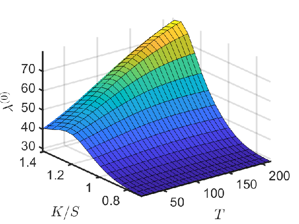
Fig. 6 shows the results for the implied $\mu$ and $\beta$ surfaces, plotted in terms of moneyness $K/S$ and time to maturity $T$ (in days), where $K$ is the strike price and $S$ is the current spot price of the underlying asset. Of the two, the $\mu$ surface has the more complex behavior with different time-development of the surface as $K/S$ ranges from “in the money” to “out of the money” values. In contrast, values of $\hat{\beta}$ decrease on both sides of a ridge of values that generally aligns with $K/S\sim 1.1$ . Values of $\beta$ , ranging from $-0.978$ to $0.147$ , are mostly negative indicating a negatively skewed pricing tree. Values of $\beta$ increase with time at any constant value of $K/S$ .

To evaluate the implied $\sigma$ surface, we also calculated the Black-Scholes implied volatility surface³³³³ 33 See Hull, 2012. $\sigma^{\textrm{(BLS)}}$ for the same option prices, and considered their difference using the percent deviation, $\textrm{Dev}^{(\alpha,\textrm{BLS})}=100\left(\sigma-\sigma^{\textrm{(BLS)}}\right)/\sigma^{\textrm{(BLS)}}$ . These surfaces are shown in Fig. 7. Both surfaces, $\sigma$ and $\sigma^{\textrm{(BLS)}}$ , show similar volatility smiles and roughly similar values when $K/S>1$ . However, the $\sigma$ surface increases more rapidly than $\sigma^{\textrm{(BLS)}}$ as $K/S$ moves deeper into the money.

4 GJR option price with hedging transaction costs

There is a vast literature on option pricing incorporating transaction costs.³⁴³⁴ 34 Some basic references are: Leland, 1985; Hodges and Neuberger, 1989; Boyle and Vorst, 1992; Davis et al., 1993; Edirisinghe et al., 1993; Kabanov and Safarian, 1997; Broadie et al., 1998; Kabanov and Stricker, 2001; Palmer, 2001; Lai and Lim, 2009; and Guasoni et al., 2012. Discrete-time option pricing models have been studied under various assumptions regarding the types of the transaction costs incurred in trading the replicating self-financing portfolios.³⁵³⁵ 35 See Merton, 1990, Stettner, 1997, Palmer, 2001, Delbaen et al., 2002, Melnikov and Petrachenko, 2005, and Chen et al., 2008. Here, we extend the GJR option pricing model to the case when the hedging is subject to transaction costs. Our approach in extending the GJR pricing tree model to include transaction costs is based on Merton’s binomial option pricing model with transaction costs.³⁶³⁶ 36 See Merton, 1990.

Consider a market with three securities $\left(\mathcal{S},\mathcal{B},\mathcal{C}\right)$ consisting of: (a) a stock $\mathcal{S}$ with pricing tree $\{S_{k\Delta t}^{(n)},\;k=1,\ldots,n,\;n\Delta t=T\}$ given by (10), (b) a bond $\mathcal{B}$ with price dynamics given by (16), and (c) an ECC $\mathcal{C}$ with price dynamics given by (17). In contrast to the previous section, we assume that the hedger (the ECC-contract seller) trades the replicating risk-neutral portfolio $P_{k\Delta t}^{(n)}=D_{k\Delta t}^{(n)}S_{k\Delta t}^{(n)}-f_{k\Delta t}^{(n)}$ at a cost. Namely, given $\mathcal{F}_{k\Delta t}=\sigma\left(M_{1}^{(\alpha_{\Delta t})},\ldots,M_{k}^{(\alpha_{\Delta t})}\right)$ , the hedged portfolio at $(k+1)\Delta t$ is determined by

	$\displaystyle P_{(k+1)\Delta t}^{(n,u,\lambda)}$	$\displaystyle=D_{k\Delta t}^{(n)}S_{(k+1)\Delta t}^{(n,u)}+\lambda_{\Delta t}D_{k\Delta t}^{(n)}\left(S_{(k+1)\Delta t}^{(n,u)}-S_{k\Delta t}^{(n)}\right)-f_{(k+1)\Delta t}^{(n,u,\lambda)},$		(22)
	$\displaystyle P_{(k+1)\Delta t}^{(n,d,\lambda)}$	$\displaystyle=D_{k\Delta t}^{(n)}S_{(k+1)\Delta t}^{(n,d)}+\lambda_{\Delta t}D_{k\Delta t}^{(n)}\left(S_{(k+1)\Delta t}^{(n,d)}-S_{k\Delta t}^{(n)}\right)-f_{(k+1)\Delta t}^{(n,d,\lambda)}.$		(22)

In (22), $\lambda_{\Delta t}=\lambda^{(0)}+\lambda^{(1)}\sqrt{\Delta t},\;\lambda^{(0)}>0$ , $\lambda^{(1)}\in R$ , is the hedging transaction cost (HTC). From (22), to leading order in $\Delta t$ , it follows that

D_{k\Delta t}^{(n)}=\frac{f_{(k+1)\Delta t}^{(n,u,\lambda)}-f_{(k+1)\Delta t}^{(n,d,\lambda)}}{2S_{k\Delta t}^{(n)}\left(1+\lambda_{\Delta t}\right)\sigma\sqrt{\Delta t}}.

(23)

As in (18) and (19), we obtain the risk-neutral valuation of the ECC,

f_{k\Delta t}^{(n,\lambda)}=D_{k\Delta t}^{(n)}S_{k\Delta t}^{(n)}-e^{-r_{f}\Delta t}P_{(k+1)\Delta t}^{(n,u,\lambda)}=e^{-r_{f}\Delta t}\left(q_{n,k+1}^{(\lambda)}f_{(k+1)\Delta t}^{(n,u,\lambda)}+(1-q_{n,k+1}^{(\lambda)})f_{(k+1)\Delta t}^{(n,d,\lambda)}\right),

(24)

where the risk-neutral probability $q_{n,k+1}^{(\lambda)}$ has the form

q_{n,k+1}^{(\lambda)}=\frac{1}{2}\left(1-\theta^{(\lambda^{(0)})}\sqrt{\Delta t}-\beta(\sqrt{1+k}-\sqrt{k})\sqrt{\frac{2\Delta t}{\pi}}\right)-\frac{\lambda^{(1)}r_{f}\Delta t}{2\sigma(1+\lambda^{(0)})^{2}},

(25)

with $\theta^{(\lambda^{(0)})}=\left(\mu+\sigma^{2}/2-r_{f}/\left(1+\lambda^{(0)}\right)\right)/\sigma$ .³⁷³⁷ 37 Formula (23) for the delta-position $D_{k\Delta t}^{(n)}$ is similar to formula (14.2a) in Merton, 1990. In the special case, $\lambda^{(0)}=\lambda^{(1)}=0$ , (25) coincides with (19).

Now consider the risk-neutral dynamics of the stock S in the presence of HTC. Conditional on $\mathcal{F}_{k\Delta t},\;k=1,\ldots,n-1$ , the risk-neutral value of the stock price at $(k+1)\Delta t$ is determined by

S_{(k+1)\Delta t}^{(n;q,\lambda)}=\begin{cases}S_{(k+1)\Delta t}^{(n,u;q,\lambda)}&=S_{k\Delta t}^{(n)}\exp\left(\mu\Delta t+\sigma\beta\left(\sqrt{k+1}-\sqrt{k}\right)\sqrt{2/\pi}\Delta t+\sigma\sqrt{\Delta t}\right),\;\textrm{w.p.}\;q_{n,k+1}^{(\lambda)},\\ S_{(k+1)\Delta t}^{(n,d;q,\lambda)}&=S_{k\Delta t}^{(n)}\exp\left(\mu\Delta t+\sigma\beta\left(\sqrt{k+1}-\sqrt{k}\right)\sqrt{2/\pi}\Delta t-\sigma\sqrt{\Delta t}\right),\;\textrm{w.p.}\;1-q_{n,k+1}^{(\lambda)},\end{cases}

(26)

where $q_{n,k+1}^{(\lambda)}$ is given by (25). Conditionally on $\mathcal{F}_{k\Delta t}$ , the discrete risk-neutral log-return $R_{(k+1)\Delta t}^{(n;q,\lambda)}=\ln\left(S_{(k+1)\Delta t}^{(n;q,\lambda)}/S_{k\Delta t}^{(n;q,\lambda)}\right)$ has mean and variance

	$\displaystyle\mathbb{E}\left(R_{(k+1)\Delta t}^{(n;q,\lambda)}\mid\mathcal{F}_{k\Delta t}\right)$	$\displaystyle=\left(\frac{r_{f}}{1+\lambda^{(0)}}-\frac{\sigma^{2}}{2}\right)\Delta t,$
	$\displaystyle\textrm{Var}\left(R_{(k+1)\Delta t}^{(n;q,\lambda)}\mid\mathcal{F}_{k\Delta t}\right)$	$\displaystyle=\sigma^{2}\Delta t.$

Setting

\mathbb{S}_{[0,T]}^{(n;q,\lambda)}=\left\{S_{t}^{(n;q,\lambda)}=S_{k\Delta t}^{(n;q,\lambda)},\;t\in[k\Delta t,(k+1)\Delta t),\;k=0,\ldots,n-1,\;S_{T}^{(n;q)}=S_{n\Delta t}^{(n)}\right\},

(27)

and

\mathbb{S}_{[0,T]}^{(q,\lambda)}=\left\{S_{0}\exp\left(\left(\frac{r_{f}}{1+\lambda^{(0)}}-\frac{\sigma^{2}}{2}\right)t+\sigma B_{t}^{(q)}\right),\;t\in[0,T]\right\},

(28)

where $\mathbb{B}_{[0,T]}^{(q)}=\left\{B_{t}^{(q)},\;t\in[0,T]\right\}$ is a standard BM, we have that $\mathbb{S}_{[0,T]}^{(n,q)}$ converges weakly in $\left(\mathcal{D}[0,T],d^{(0)}\right)$ to $\mathbb{S}_{[0,T]}^{(q)}$ . From (28), it follows that the value of $\lambda^{(1)}$ in the HTC is irrelevant in continuous-time trading. However, for every fixed $\Delta t$ , the risk-neutral tree (20) will exhibit the behavior of a geometric SBM and the value of $\lambda^{(1)}$ becomes relevant, as evident from (24).

Remark: It appears natural to assume that HTC could be asymmetric; that is, instead of (22), we could assume that

	$\displaystyle P_{(k+1)\Delta t}^{(n,u,\lambda)}$	$\displaystyle=D_{k\Delta t}^{(n)}S_{(k+1)\Delta t}^{(n,u)}+\lambda^{(u)}_{\Delta t}D_{k\Delta t}^{(n)}\left(S_{(k+1)\Delta t}^{(n,u)}-S_{k\Delta t}^{(n)}\right)-f_{(k+1)\Delta t}^{(n,u,\lambda)},$		(29)
	$\displaystyle P_{(k+1)\Delta t}^{(n,d,\lambda)}$	$\displaystyle=D_{k\Delta t}^{(n)}S_{(k+1)\Delta t}^{(n,d)}+\lambda^{(d)}_{\Delta t}D_{k\Delta t}^{(n)}\left(S_{(k+1)\Delta t}^{(n,d)}-S_{k\Delta t}^{(n)}\right)-f_{(k+1)\Delta t}^{(n,d,\lambda)},$		(29)

with $\lambda_{\Delta t}^{(u)}\neq\lambda_{\Delta t}^{(d)}$ , where

	$\displaystyle\lambda_{\Delta t}^{(u)}$	$\displaystyle=\lambda^{(0,u)}+\lambda^{(1,u)}\sqrt{\Delta t},\;\lambda^{(0,u)}>0,\;\lambda^{(1,u)}\in R,$
	$\displaystyle\lambda_{\Delta t}^{(d)}$	$\displaystyle=\lambda^{(0,d)}+\lambda^{(1,d)}\sqrt{\Delta t},\;\lambda^{(0,d)}>0,\;\lambda^{(1,d)}\in R.$

A close inspection shows that, as $\Delta t\downarrow 0$ , (29) leads to a pricing model which is not arbitrage free. However, for fixed $\Delta t$ , the model (29) is arbitrage free and an expression for the risk-neutral probability $q_{n,k+1}^{(\lambda)}$ similar to formula (24) can be readily obtained.³⁸³⁸ 38 Discrete-time market models, which are free of arbitrages, but for which the corresponding continuous-time market model is not arbitrage-free, are known; see, for example, Karandikar and Rachev, 1995 and Hurst et al., 1999. In those models, the discrete equivalent martingale measure explodes in the limit. Similarly, if we assume that (29) holds, the limiting martingale measure does not exist.

4.1 Implied surfaces with the inclusion of HTC

As in section 3.1, we numerically illustrate the HTC and its limiting behavior using the same data set, including closing and call option prices, for the underlying asset SPY . Following the notation in section 3.1, we set the parameter $\rho=\rho^{(\lambda)}=\left(\lambda^{(0)},\lambda^{(1)}\;|\;\bar{\mu}^{(\alpha)},\bar{\beta}^{(\alpha)},\bar{\sigma}^{(\alpha)}\right)$ . From (24), (25) and (26), we construct the GJR tree option price $C_{i}^{(\textrm{SPY,GJR})}(\rho^{(\lambda)})$ . We find the optimal solution for $\rho^{(\lambda)}$ by minimizating the relative mean-square error (relMSE)

\min_{\lambda^{(0)}>0,\;\lambda^{(1)}\in R}\;\textrm{relMSE}=\min_{\lambda^{(0)}>0,\;\lambda^{(1)}\in R}\frac{1}{M}\sum_{i=1}^{M}\left(\frac{C_{i}^{(\textrm{SPY,GJR})}\left(\rho\right)-C_{i}^{(\textrm{SPY,Market})}}{C_{i}^{(\textrm{SPY,Market})}}\right)^{2}.

(30)

The resulting minimizing values are $\textrm{relMSE}=0.433$ for $\lambda^{(0)}=28.8$ and $\lambda^{(1)}=0.297$ .³⁹³⁹ 39 The three terms on the right-hand side of (22) have the form $DS+\lambda D\Delta S-f$ , where the transaction cost term is $\lambda D\Delta S$ . The estimated values of $\lambda^{(0)}$ and $\lambda^{(1)}$ yield $\lambda\approx\lambda^{(0)}=28.8$ . If daily stock price changes for the SPY fund are around 0.1% of the fund price (i.e. $\Delta S\sim 10^{-3}S$ ), the transaction cost term would have the value $0.0288DS$ , indicating transactions costs contribute $\sim$ 3% to the total price of the hedged portfolio. Using the parameters $\rho^{(\lambda^{(0)})}=(\lambda^{(0)}\;|\;\bar{\mu}^{(\alpha)},\bar{\beta}^{(\alpha)},\bar{\sigma}^{(\alpha)},\lambda^{(1)}=0.297)$ and $\rho^{(\lambda^{(1)})}=(\lambda^{(1)}\;|\;\bar{\mu}^{(\alpha)},\bar{\beta}^{(\alpha)},\bar{\sigma}^{(\alpha)},\linebreak\lambda^{(0)}=28.8)$ , we reran the minimization problem (21) and computed the $\lambda^{(0)}$ and $\lambda^{(1)}$ surfaces shown in Fig. 8. Both surfaces have a similar ridge shape, but of vastly different scales. The value of $\lambda^{(1)}$ is constant through five computed digits, whereas $\lambda^{(0)}$ varies significantly in the first computed digit. Thus, for these values of $\bar{\mu}^{(\alpha)}$ , $\bar{\beta}^{(\alpha)}$ and $\bar{\sigma}^{(\alpha)}$ , the constant value model, $\lambda_{\Delta t}=\lambda^{(0)}$ , would suffice in (22).

To ascertain the effects of adding HTC, we computed the implied $\mu$ , $\beta$ , and $\sigma$ surfaces using the minimizing values for $\lambda^{(0)}$ and $\lambda^{(1)}$ . (For example, for the $\mu$ surface we estimated values for $\rho^{(\mu)}=(\mu\ |\ \bar{\sigma}^{(\alpha)}=0.151,\bar{\beta}^{(\alpha)}=-0.978,\lambda^{(0)}=28.8,\lambda^{(1)}=0.297)$ using (21).) To compare the results with those reported in section 3.1, we also computed the percent deviation surfaces, $\rho^{(\textrm{dev})}=100\left(\rho^{(\textrm{HTC})}-\rho^{(\textrm{GJR})}\right)/\rho^{(\textrm{GJR})}$ for $\rho=\{\mu,\sigma\}$ , where $\rho^{(\textrm{GJR})}$ refers to the surface computed for the GJR model without HTC in section 3.1 and $\rho^{(\textrm{HTC})}$ refers to the surface computed for the GJR model with HTC. To avoid division by zero, for the $\beta$ surface comparison we plot the difference surface $\beta^{(\textrm{diff})}=\beta^{(\textrm{HTC})}-\beta^{(\textrm{GJR})}$ . The results are shown in Fig. 9. Inclusion of HTC has the effect of differentially lowering $\mu$ values (as expected since the trader is expending money on fees), most noticeably along the coordinate $K/S\sim 1.2$ . Similarly expected, inclusion of HTC differentially raises the volatility surface. HTC differentially raises $\beta$ values, with greater increases arising as $K/S$ values move more “into the money”, resulting in larger regions of the phase space where the pricing tree is positively skewed.

5 Fitting the GJR pricing tree to a market driver

In this section we explore possibilities for fitting the pricing tree model, $S_{k\Delta t}^{(n)}$ , $k=1,\ldots,n$ , to a market driver that affects the price dynamics, $S_{k\Delta t}^{(n,\mathcal{S})}$ , of stock $\mathcal{S}$ . We consider both endogenous and exogenous approaches. In the endogenous approach, the discrete dynamics for the price of $\mathcal{S}$ is modeled by

	$\displaystyle S_{k\Delta t}^{(n,\textrm{endo})}$	$\displaystyle=S_{0}\exp\left(v_{k}^{(0,\mathcal{S})}\Delta t+M_{k}^{(\textrm{endo})}\sigma^{(0,\mathcal{S})}\sqrt{\Delta t}\right),$		(31)
	$\displaystyle v_{k}^{(0,\mathcal{S})}$	$\displaystyle=k\mu^{(0,\mathcal{S})}+\sigma^{(0,\mathcal{S})}\beta^{(0,\mathcal{S})}\left(\sqrt{2k/\pi}-1\right),\;k=1,\ldots,n,$

with the path $M_{1}^{(\textrm{endo})},\ldots,M_{k}^{(\textrm{endo})}$ of the Markov chain $\mathbb{M}^{(\textrm{endo})}$ determined by⁴⁰⁴⁰ 40 Here $\textrm{sign}(x)=\begin{cases}1,\;\textrm{if}\;x\geq 0\\ -1,\;\textrm{if}\;x<0\end{cases}$ .

M_{k}^{(\textrm{endo})}=\sum_{j=1}^{k}\textrm{sign}\left(r_{j\Delta t}^{(n,\mathcal{S})}\right),\ j=1,\dots,k;\ M_{0}^{(\textrm{endo})}=0,

where $r_{j\Delta t}^{(n,\mathcal{S})}=\ln\left(S_{j\Delta t}^{(n,\mathcal{S})}/S_{(j-1)\Delta t}^{(n,\mathcal{S})}\right)$ is the market’s daily log-return for stock $\mathcal{S}$ . In (31), the parameters $\sigma^{(0,\mathcal{S})}$ , $\mu^{(0,\mathcal{S})}$ and $\beta^{(0,\mathcal{S})}$ are determined for the initial time $k\Delta t=0$ from equations (14) and (15) using the cumulative return data for $\mathcal{S}$ applicable at the chosen start date $k\Delta t=0$ . The values obtained from (14) and (15) are also smoothed using the moving-window averaging procedure introduced in section 2.4. This will be demonstrated explicitly by numerical example in section 5.1.

The endogenous approach is limited while the exogenous approach assumes that the $M_{k}^{(\alpha_{\Delta t})}$ are determined by the upward and downward movements of a more general market driver. For concreteness, we initially assume the market driver is a factor model for the price dynamics of $\mathcal{S}$ ; in particular we consider the Fama-French five-factor asset pricing model.

Fama-French five-factor model.⁴¹⁴¹ 41 See Fama and French (2012, 2015, 2017). With $r_{j\Delta t}^{(n,\mathcal{S})}$ being the market log-return of stock $\mathcal{S}$ for the period $[j\Delta t,(j+1)\Delta t)$ , the coefficients of the terms in the Fama-French factor return,

r_{j\Delta t}^{(n,F)}=r_{f,j\Delta t}+\mathbbm{a}+\mathbbm{b}\left(r_{j\Delta t}^{(n,M)}-r_{f,j\Delta t}\right)+\mathbbm{s}r_{j\Delta t}^{(n,SMB)}+\mathbbm{h}r_{j\Delta t}^{(n,HML)}+\mathbbm{r}r_{j\Delta t}^{(n,RMW)}+\mathbbm{c}r_{j\Delta t}^{(n,CMA)},

(32)

are determined from the regression

r_{j\Delta t}^{(n,\mathcal{S})}=r_{j\Delta t}^{(n,F)}+\epsilon_{j\Delta t},\quad j=0,1,\ldots,m-1.

(33)

In (32), $r_{f,j\Delta t}$ is the risk-free rate in period $[j\Delta t,(j+1)\Delta t)$ and the remaining Fama-French factors are:

$\mathbb{F}_{1}$ :

$r_{j\Delta t}^{(n,M)}$ (representing the market-factor effect) is the return over the period $[j\Delta t,(j+1)\Delta t)$ of the capitalization weighted stock market to which $\mathcal{S}$ belongs;
$\mathbb{F}_{2}$ :

$r_{j\Delta t}^{(n,SMB)}$ (representing the size-factor effect) is the difference in the return of a portfolio in $\mathcal{M}$ specializing in (a) small-cap and (b) large-cap stocks;
$\mathbb{F}_{3}$ :

$r_{j\Delta t}^{(n,HML)}$ (representing the value-factor effect) is the difference of the returns of a portfolio in $\mathcal{M}$ with (a) high and (b) small book-to-market ratios;
$\mathbb{F}_{4}$ :

$r_{j\Delta t}^{(n,RMW)}$ (representing the profitability-premium-factor effect) is the difference of the return of a portfolio in $\mathcal{M}$ with (a) high and (b) low profitability; and
$\mathbb{F}_{5}$ :

$r_{j\Delta t}^{(n,CMA)}$ (representing the investment-attitude-factor effect) is the difference of the return of a portfolio of stocks in $\mathcal{M}$ issued by firms that invest (a) conservatively and (b) aggressively.

Let $j\Delta t$ , $j=1,\dots,m$ denote a time period $\tau_{1}$ and $j=m+1,\dots,m+n$ denote the following time period $\tau_{2}$ . Let $\hat{r}_{j\Delta t}^{(n,F)}$ , $j=1,\ldots,m$ , denote sample return values (factor returns) for (32) obtained from the regression (33) over the period $\tau_{1}$ , and $\hat{R}_{j\Delta t}^{(n,F)}$ denote the resultant cumulative factor returns. Using the cumulative factor returns on the left-hand side of (14) and (15), and the moving-window averaging procedure introduced in section 2.4, we obtain estimates $\bar{\sigma}^{(F)}$ , $\bar{\mu}^{(F)}$ and $\bar{\beta}^{(F)}$ for the values of the parameters $\sigma$ , $\mu$ and $\beta$ at timestep $m\Delta t$ . Let $k\Delta t$ , $k=1,\dots,n$ , where $k=j-m$ , label the trading days in time period $\tau_{2}$ . Then $\bar{\sigma}^{(F)}$ , $\bar{\mu}^{(F)}$ and $\bar{\beta}^{(F)}$ correspond to parameter values for $k\Delta t=0$ .

We model the discrete dynamics for the factor-driven price over the period $\tau_{2}$ by

	$\displaystyle S_{k\Delta t}^{(n,\textrm{exo})}$	$\displaystyle=S_{0}\exp\left(v_{k}^{(F)}\Delta t+M_{k}^{\left(\bar{\alpha}^{(F)},\textrm{exo}\right)}\bar{\sigma}^{(F)}\sqrt{\Delta t}\right),$		(34)
	$\displaystyle v_{k}^{(F)}$	$\displaystyle=k\bar{\mu}^{(F)}+\bar{\sigma}^{(F)}\bar{\beta}^{(F)}\left(\sqrt{2k/\pi}-1\right),$

where $\bar{\alpha}^{(F)}_{\Delta t}=(1+\bar{\beta}^{(F)}\sqrt{\Delta t})/2$ . To estimate the path $M_{k}^{\left(\bar{\alpha}^{(F)},\textrm{exo}\right)}$ , we generate a large ensemble of sample paths $\left\{M_{k}^{\left(\bar{\alpha}^{(F)}\right)},\ k=1,\dots,n\right\}$ . $M_{k}^{\left(\bar{\alpha}^{(F)},\textrm{exo}\right)}$ is then chosen as that path that minimizes the relMSE between the two sides of (34) when the stock prices $S_{k\Delta t}^{(n,\mathcal{S})}$ are used on the left-hand side of (34). This exogenous method is also demonstrated in section 5.1.

5.1 Numerical example of the endogenous and exogenous approaches

We demonstrate the endogenous and exogenous approaches using the daily return series for the stock $\mathcal{S}=\textrm{MSFT}$ . The price data set⁴²⁴² 42 MSFT market closing prices from Bloomberg Professional Services. Return values for the Fama-French factors from the U.S. Research Returns Data Center (https://mba.tuck.dartmouth.edu/pages/faculty/ken.french/Data_Library.html). covers the period 4/30/2015 tthrough 4/30/2021. Since the estimation (equations (14) and (15)) and averaging procedures of section 2.4 for $\sigma$ , $\mu$ and $\beta$ require one-year moving windows, we divide the data set into two time periods, $\tau_{1}=$ 4/31/2015 through 4/28/2017 and $\tau_{2}=$ 5/1/2017 through 4/30/2021. MSFT data on the close of 4/28/2017 in $\tau_{1}$ serves as $t=0$ data for $\tau_{2}$ ; the closing price of MSFT on 4/28/2017 serves as $S_{0}$ for the period $\tau_{2}$ and cumulative returns over $\tau_{2}$ are then computed relative to this $S_{0}$ . And applying the estimation and averaging procedures of section 2.4 to the cumulative log-return data for MSFT over $\tau_{1}$ , we obtain estimates $\bar{\sigma}^{(0,\textrm{MSFT})}$ , $\bar{\mu}^{(0,\textrm{MSFT})}$ and $\bar{\beta}^{(0,\textrm{MSFT})}$ determined for the close of trading on 4/28/2017. These values, along with $\bar{\alpha}^{(0,\textrm{MSFT})}$ and the value of the relMSE, are given in Table 1. Using $\bar{\sigma}^{(0,\textrm{MSFT})}$ , $\bar{\mu}^{(0,\textrm{MSFT})}$ and $\bar{\beta}^{(0,\textrm{MSFT})}$ in (31) we obtain an endogenous estimate $S_{k\Delta t}^{(n,\textrm{endo})}$ for the cumulative price dynamics of MSFT over the period $\tau_{2}$ .

endogenous	$\bar{\mu}^{(0,\textrm{MSFT})}$	$\bar{\sigma}^{(0,\textrm{MSFT})}$	$\bar{\beta}^{(0,\textrm{MSFT})}$	$\bar{\alpha}^{(0,\textrm{MSFT})}$	relMSE
endogenous	$7.38\cdot 10^{-4}$	$8.91\cdot 10^{-2}$	$-4.08$	0.371	$1.78\cdot 10^{-3}$
exogenous	$\bar{\mu}^{(F)}$	$\bar{\sigma}^{(F)}$	$\bar{\beta}^{(F)}$	$\bar{\alpha}^{(F)}$	relMSE
exogenous	$2.31\cdot 10^{-4}$	$7.01\cdot 10^{-3}$	$-11.2$	0.147	$3.22\cdot 10^{-3}$

Table 1: Parameters estimates from the endogenous and exogenous estimation procedures

For the exogenous approach, we use the Fama-French five-factor model outlined in the previous section as the market driver. The Fama-French factor returns, $r_{k\Delta t}^{(n,F)}$ in (32), were computed over the period $\tau_{1}$ using a robust form for the regression (33).⁴³⁴³ 43 Motivated by results in Knez and Ready, 1997, we choose robust regression in estimating the parameters of the Fama-French five-factor model. The values of the coefficients, as well as the R-square and root mean square-error (RMSE) values, are given in Table 2. The sample return $\hat{r}^{(n,F)}_{k\Delta t}$ and price $\hat{S}^{(n,F)}_{k\Delta t}$ series computed from these coefficients are presented in Fig. 10 where they are compared with the market return $r^{(n,\textrm{MSFT})}_{k\Delta t}$ and price $S^{(n,\textrm{MSFT})}_{k\Delta t}$ series over the period $\tau_{1}$ . The significant differences between the series $\hat{S}^{(n,F)}_{k\Delta t}$ and $S^{(n,\textrm{MSFT})}_{k\Delta t}$ are indicative of issues with applying market driver analyses to stock returns. Since the Fama-French model is based upon a regression fit to return values, errors produced in return values have large-time decay structure and lead ultimately to significant cumulative differences in price performance.

$\mathbbm{a}$	$\mathbbm{b}$	$\mathbbm{s}$	$\mathbbm{h}$	$\mathbbm{r}$	$\mathbbm{c}$	R-square	RMSE
$-6.5\cdot 10^{-4}$	$1.2\cdot 10^{-2}$	$-3.9\cdot 10^{-3}$	$-4.0\cdot 10^{-4}$	$3.0\cdot 10^{-3}$	$-5.8\cdot 10^{-3}$	0.58	$9.1\cdot 10^{-3}$

Table 2: Parameter estimates from the regression (33)

The parameter estimates $\bar{\mu}^{(F)}$ , $\bar{\sigma}^{(F)}$ , $\bar{\beta}^{(F)}$ , and $\bar{\alpha}^{(F)}$ obtained for 4/28/2017 using the cumulative Fama-French returns over $\tau_{1}$ are given in Table 1. These values generally differ by a factor of $\sim 3$ compared to the corresponding endogenous variables, with the exception of a factor of $\sim 13$ difference between $\bar{\sigma}^{(F)}$ and $\bar{\sigma}^{(0,\textrm{MSFT})}$ . Using the estimated value $\bar{\alpha}^{(F)}$ , we generate $10^{6}$ scenarios of the sample path $M_{k}^{\left(\bar{\alpha}^{(F)}\right)}$ covering the time period $\tau_{2}$ . Using the price data $S_{k\Delta t}^{(n,\textrm{MSFT})}$ for $\tau_{2}$ on the left-hand side of (34), the optimal path $M_{k}^{\left(\bar{\alpha}^{(F)},\textrm{exo}\right)}$ was selected as the path scenario that minimized the relMSE between the left- and right-hand sides. The exogenous price series estimate $S_{k\Delta t}^{(n,\textrm{exo})}$ for $\tau_{2}$ is then computed from (34) using $M_{k}^{\left(\bar{\alpha}^{(F)},\textrm{exo}\right)}$ on the right-hand side.

The cumulative price $S_{k\Delta t}^{(n,\textrm{MSFT})}$ over $\tau_{2}$ is compared with the estimates $S_{k\Delta t}^{(n,\textrm{endo})}$ and $S_{k\Delta t}^{(n,\textrm{exo})}$ in Fig. 11. Both estimates produce reasonable agreement to the actual price data; however both significantly smooth and decrease the impact of the Covid-19 pandemic; the exogenous method showing less impact from the pandemic than the endogenous method.

5.2 Inclusion of the higher moment SBM process $\mathbb{C}_{t}^{(\alpha,n)}$

For a general market driver, we extend to the full functionality of the CYSIP by adding the higher moment SBM process $\mathbb{C}_{t}^{(\alpha,n)}$ into our model.⁴⁴⁴⁴ 44 See Hu et al., 2020b for an application of the CSYIP using BM. According to (34), $S_{k\Delta t}^{(n,\textrm{exo})}$ is adapted to the filtration

\mathbb{F}^{(n;\mathbb{M}^{(\alpha_{\Delta t})})}=\left\{\mathcal{F}_{k}^{(n;\mathbb{M}^{(\alpha_{\Delta t})})}=\sigma\left(M_{j}^{(\alpha_{\Delta t})};\;j=1,\ldots,k\right),\;k=1,\ldots,n,\;\mathcal{F}_{k}^{(n;\mathbb{M}^{(\alpha_{\Delta t})})}=\left\{\varnothing,\Omega\right\}\right\}.

Paralleling the development for the lower moment SBM process in section 2.2, with $n\Delta t=T$ we set $M_{0}^{(\alpha_{\Delta t},n)}=0$ , $M_{k}^{(\alpha_{\Delta t},n)}=n^{-1/2}M_{k}^{(\alpha_{\Delta t})}$ , and $X_{k/n}^{(\alpha_{\Delta t},n)}=\sum_{i=1}^{k}M_{i}^{(\alpha_{\Delta t},n)},\;k=1,\ldots,n$ . Let $B_{t}^{(\alpha_{\Delta t},n)},\;t\geq 0$ be a random process with piecewise linear trajectories having vertexes $\left(k/n,\mathbb{B}_{k/n}^{(\alpha_{\Delta t},n)}\right),\;k=1,\ldots,n$ , where $\mathbb{B}_{k/n}^{(\alpha_{\Delta t},n)}=X_{k/n}^{(\alpha_{\Delta t},n)}$ . Let $h:R\rightarrow R$ be a piecewise continuous function and define $Y_{k/n}^{(\alpha_{\Delta t},n)}=\sum_{i=1}^{k}h\left(X_{(i-1)/n}^{(\alpha_{\Delta t},n)}\right)\left(X_{i/n}^{(\alpha_{\Delta t},n)}-X_{(i-1)/n}^{(\alpha_{\Delta t},n)}\right),\;k\in\mathcal{N},\;n\in\mathcal{N}$ . Define $\mathbb{C}_{t}^{(\alpha_{\Delta t},n;h)},\;t\geq 0$ to be a random process with the piecewise linear trajectories having vertexes $\left(k/n,\mathbb{C}_{k/n}^{(\alpha_{\Delta t},n;h)}\right),\;k\in\mathcal{N},\;n\in\mathcal{N}$ , where $\mathbb{C}_{k/n}^{(\alpha_{\Delta t},n;h)}=Y_{k/n}^{(\alpha_{\Delta t},n;h)}$ . Then, for a fixed, relatively small value of $\Delta t$ , the bivariate process $\left(\mathbb{B}_{t}^{(\alpha_{\Delta t},n)},\mathbb{C}_{t}^{(\alpha_{\Delta t},n;h)}\right),\;t\geq 0$ , approaches $\left(B_{t}^{(\alpha_{\Delta t})},C_{t}^{(\alpha_{\Delta t};h)}\right)$ , where $B_{t}^{(\alpha_{\Delta t})}$ is a SBM and $C_{t}^{(\alpha_{\Delta t};h)}=\int_{0}^{t}h\left(B_{s}^{(\alpha_{\Delta t})}\right)dB_{s}^{(\alpha_{\Delta t})}$ . However, as $n\uparrow\infty$ and $\Delta t\downarrow 0,\;\left(\mathbb{B}_{t}^{(\alpha_{\Delta t},n)},\mathbb{C}_{t}^{(\alpha_{\Delta t},n)}\right)$ converges in law to $\left(B_{t},C_{t}\right)$ for $t\geq 0$ , where $B_{t}$ is a BM and $C_{t}=\int_{0}^{t}h\left(B_{s}\right)dB_{s}$ .⁴⁵⁴⁵ 45 See Cherny et al., 2003.

Next, consider the following two processes in $\mathcal{D}[0,T]$ :

	$\displaystyle\mathbb{B}_{[0,T]}^{(\alpha_{\Delta t},n)}$	$\displaystyle=\left\{\mathbb{B}_{t}^{(\alpha_{\Delta t},n)}=\sqrt{T}X_{k/n}^{(\alpha_{\Delta t},n)},\;t\in[k\Delta t,(k+1)\Delta t),\;\mathbb{B}_{1}^{(\alpha_{\Delta t},n)}=X_{1}^{(\alpha_{\Delta t},n)}\right\},$
	$\displaystyle\mathbb{C}_{[0,T]}^{(\alpha_{\Delta t},n,h)}$	$\displaystyle=\left\{\begin{aligned} \mathbb{C}_{t}^{(\alpha_{\Delta t},n;h)}&=\sum_{i=1}^{k}h\left(\sqrt{T}X_{(i-1)/n}^{(\alpha_{\Delta t},n)}\right)\left(\sqrt{T}X_{i/n}^{(\alpha_{\Delta t},n)}-\sqrt{T}X_{(i-1)/n}^{(\alpha_{\Delta t},n)}\right),\;t\in[k\Delta t,(k+1)\Delta t),\\ \mathbb{C}_{1}^{(\alpha_{\Delta t},n)}&=Y_{1}^{(\alpha_{\Delta t},n)}\end{aligned}\right\}.$

Then, for large $n$ , the bivariate process $\left(\mathbb{B}_{[0,T]}^{(\alpha_{\Delta t},n)},\mathbb{C}_{[0,T]}^{(\alpha_{\Delta t},n;h)}\right)$ approaches $\left(\mathbb{B}_{[0,T]}^{(\alpha_{\Delta t})},\mathbb{C}_{[0,T]}^{(\alpha_{\Delta t};h)}\right)$ in $\mathcal{D}[0,T]\cdot\mathcal{D}[0,T]$ , where $\mathbb{B}_{[0,T]}^{(\alpha_{\Delta t})}=\left\{B_{t}^{(\alpha_{\Delta t})},\;t\in[0,T]\right\}$ is a SBM on $[0,T]$ and $\mathbb{C}_{[0,T]}^{(\alpha_{\Delta t};h)}=\left\{C_{t}^{(\alpha_{\Delta t};h)},\;t\in[0,T]\right\}$ . Ultimately, as $n\uparrow\infty$ , $\left(\mathbb{B}_{[0,T]}^{(\alpha_{\Delta t},n)},\mathbb{C}_{[0,T]}^{(\alpha_{\Delta t},n;h)}\right)$ converges weakly in $\mathcal{D}[0,T]\cdot\mathcal{D}[0,T]$ to $\left(\mathbb{B}_{[0,T]},\mathbb{C}_{[0,T]}^{(h)}\right)$ , where $\mathbb{B}_{[0,T]}=\left\{B_{t},\;t\in[0,T]\right\}$ is a BM on $[0,T]$ and $\mathbb{C}_{[0,T]}^{(h)}=\left\{C_{t}^{(h)}=\int^{t}_{0}h\left(B_{s}\right)dB_{s},\;t\in[0,T]\right\}$ .

Now define the stock price discrete dynamics as a functional of $\mathbb{B}_{[0,T]}^{(\alpha_{\Delta t},n)}$ and $\mathbb{C}_{[0,T]}^{(\alpha_{\Delta t},n;h)}$ . Let

\mathbb{S}_{[0,T]}^{(\alpha_{\Delta t},n;h)}=\left\{\begin{aligned} S_{t}^{(\alpha_{\Delta t},n;h)}&=S_{0}\exp\left(vk\Delta t+\sigma\mathbb{B}_{t}^{(\alpha_{\Delta t},n)}+\gamma\mathbb{C}_{t}^{(\alpha_{\Delta t},n;h)}\right),\;t\in[k\Delta t,(k+1)\Delta t),k=1,\ldots,n,\\ S_{T}^{(\alpha_{\Delta t},n;h)}&=S_{0}\exp\left(vT+\sigma\mathbb{B}_{T}^{(\alpha_{\Delta t},n)}+\gamma\mathbb{C}_{T}^{(\alpha_{\Delta t},n;h)}\right)\end{aligned}\right\},

(35)

where $v\in R$ , $\sigma\in R\backslash\{0\}$ and $\gamma\in R$ are parameters determining the dynamics of the stock price as a function of the index dynamics. The discrete dynamics of the stock log-return is given by

r_{k\Delta t}^{(\alpha_{\Delta t},n;h)}=\ln\left(\frac{S_{k\Delta t}^{(\alpha_{\Delta t},n;h)}}{S_{(k-1)\Delta t}^{(\alpha_{\Delta t},n;h)}}\right)=v\Delta t+\sigma\sqrt{\Delta t}M_{k}^{(\alpha_{\Delta t})}+\gamma\sqrt{\Delta t}M_{k}^{(\alpha_{\Delta t})}h\left(\sum_{i=1}^{k-1}\sqrt{\Delta t}M_{i}^{(\alpha_{\Delta t})}\right),k=1,\ldots,n.

(36)

Thus, if $\gamma\neq 0$ , the stock log-return $r_{k\Delta t}^{(\alpha_{\Delta t},n;h)}$ depends on the entire path $\{M_{i}^{(\alpha_{\Delta t})},\;i=1,\ldots,k\}$ . In the pre-limiting case, $\mathbb{S}_{[0,T]}^{(\alpha_{\Delta t},n;h)}$ approaches $\mathbb{S}_{[0,T]}^{(\alpha_{\Delta t};h)}=\{S_{0}\exp\left(vt+\sigma B_{t}^{(\alpha_{\Delta t})}+\gamma C_{t}^{(\alpha_{\Delta t};h)}\right),\;t\in[0,T]\}$ . In the limit $n\uparrow\infty$ , $\mathbb{S}_{[0,T]}^{(\alpha_{\Delta t},n;h)}$ converges weakly in $\mathcal{D}[0,T]$ to $\mathbb{S}_{[0,T]}^{(h)}=\{S_{0}\exp\left(vt+\sigma B_{t}+\gamma C_{t}^{(h)}\right),\;t\in[0,T]\}$ .

To demonstrate the application of the model (35), (36), we use (36) to estimate the MSFT log-return $r_{k\Delta t}^{(n,\textrm{MSFT})}$ over the period $\tau_{2}$ . To capture likely heavy-tailed behavior, we identify $h(\cdot)$ as the Student’s $t$ probability density function with $\kappa$ degrees of freedom. For convenience, we utilize the optimal path $M_{k}^{\left(\bar{\alpha}^{(F)},\textrm{exo}\right)}$ determined from the exogenous procedure in section 5.1 for the required path in (36). To establish the model parameters, $v$ , $\sigma$ , $\gamma$ , and $\kappa$ , we construct the conditional least squares minimization problem,

\min_{\nu\in R,\sigma\in R,\gamma\in R,\kappa\in[5,30]}\parallel r_{k\Delta t}^{(n,\textrm{MSFT})}-r_{k\Delta t}^{(\alpha_{\Delta t},n;h)}\parallel_{2}^{2}.

(37)

Table 3 provides the resulting parameter estimates. The model (35), (36) with these parameter estimates will be used further in section 6.1.

$v$	$\sigma$	$\gamma$	$\kappa$	RMSE
0.272	$3.44\cdot 10^{-5}$	$4.22\cdot 10^{-2}$	6.24	$1.86\cdot 10^{-2}$

Table 3: Parameters estimates obtained from (37)

6 GJR option pricing

Given the filtration $\mathbb{F}^{(n;\mathbb{M}^{(\alpha_{\Delta t})})}=\{\mathcal{F}_{k}^{(n;\mathbb{M}^{(\alpha_{\Delta t})}}=\sigma\left(M_{j}^{(\alpha_{\Delta t})};j=1,\ldots,k\right),\;\mathcal{F}_{k}^{(n;\mathbb{M}^{(\alpha_{\Delta t})})}=\{\varnothing,\Omega\},\;k=1,\ldots,n\}$ , consider the $\mathbb{F}^{(n;\mathbb{M}^{(\alpha_{\Delta t})})}$ -adapted path-dependent GJR pricing tree determined by (36),

S_{k\Delta t}^{(\alpha_{\Delta t},n;h)}=S_{(k-1)\Delta t}^{(\alpha_{\Delta t},n;h)}\exp\left[v\Delta t+\sigma\sqrt{\Delta t}\left(M_{k}^{(\alpha_{\Delta t})}-M_{k-1}^{(\alpha_{\Delta t})}\right)\right.\\ \left.+\gamma\sqrt{\Delta t}\left(M_{k}^{(\alpha_{\Delta t})}-M_{k-1}^{(\alpha_{\Delta t})}\right)h\left(\sqrt{\Delta t}M_{k-1}^{(\alpha_{\Delta t})}\right)\right),

(38)

where $k=1,\ldots,n,\;n\Delta t=T$ . Let $h(x)\geq 0,\;x\in R$ , be a chosen probability density function.⁴⁶⁴⁶ 46 For example, $h$ is the Student’s $t$ density function with $\kappa$ -degrees of freedom. Define

\eta_{k\Delta t}=\sigma+\gamma h\left(\sqrt{\Delta t}M_{k-1}^{(\alpha_{\Delta t})}\right),\;k=1,\ldots,n;\qquad\eta_{0}=\sigma.

(39)

Note that $\eta_{k\Delta t}^{(\alpha_{\Delta t})}$ represents the stock’s time-varying factor-volatility at $k\Delta t$ as a function of the path of factor up and down movements $M_{k-1}^{(\alpha_{\Delta t})}$ . From (38), conditionally on $\mathcal{F}_{k}^{(n;\mathbb{M}^{(\alpha_{\Delta t})})},\;k=0,\ldots,n-1,$

S_{(k+1)\Delta t}^{(\alpha_{\Delta t},n;h)}=\begin{cases}S_{(k+1)\Delta t}^{(\alpha_{\Delta t},n,u;h)}&=S_{k\Delta t}^{(\alpha_{\Delta t},n;h)}\exp\left(v\Delta t+\eta_{k\Delta t}^{(\alpha_{\Delta t})}\sqrt{\Delta t}\right),\;\textrm{w.p.}\;\mathbb{P}\left(M_{k+1}^{(\alpha)}=M_{k}^{(\alpha)}+1\mid M_{k}^{(\alpha)}\right),\\ S_{(k+1)\Delta t}^{(\alpha_{\Delta t},n,d;h)}&=S_{k\Delta t}^{(\alpha_{\Delta t},n;h)}\exp\left(v\Delta t-\eta_{k\Delta t}^{(\alpha_{\Delta t})}\sqrt{\Delta t}\right),\;\textrm{w.p.}\;\mathbb{P}\left(M_{k+1}^{(\alpha)}=M_{k}^{(\alpha)}-1\mid M_{k}^{(\alpha)}\right).\end{cases}

(40)

For $k=0,1,\ldots,n-1$ , consider the replicating risk-neutral portfolio $P_{k\Delta t}^{(\alpha_{\Delta t},n;h)}=S_{k\Delta t}^{(\alpha_{\Delta t},n;h)}D_{k\Delta t}^{(\alpha_{\Delta t},n;h)}-f_{k\Delta t}^{(\alpha_{\Delta t},n;h)}$ with $P_{(k+1)\Delta t}^{(\alpha_{\Delta t},n;h)}=S_{(k+1)\Delta t}^{(\alpha_{\Delta t},n;h)}D_{k\Delta t}^{(\alpha_{\Delta t},n;h)}-f_{(k+1)\Delta t}^{(\alpha_{\Delta t},n;h)}$ , given $\mathcal{F}_{k}^{(n;\mathbb{M}^{(\alpha_{\Delta t})})}$ . Thus, conditionally on $\mathcal{F}_{k}^{(n;\mathbb{M}^{(\alpha_{\Delta t})})}$ ,

D_{k\Delta t}^{(\alpha_{\Delta t},n;h)}=\frac{f_{(k+1)\Delta t}^{(\alpha_{\Delta t},n,u;h)}-f_{(k+1)\Delta t}^{(\alpha_{\Delta t},n,d;h)}}{e^{v\Delta t}S_{k\Delta t}^{(\alpha_{\Delta t},n;h)}\left(\exp\left(\eta_{k\Delta t}^{(\alpha_{\Delta t})}\sqrt{\Delta t}\right)-\exp\left(-\eta_{k\Delta t}^{(\alpha_{\Delta t})}\sqrt{\Delta t}\right)\right)}.

As portfolio $P_{(k+1)\Delta t}^{(\alpha_{\Delta t},n;h)}$ is now riskless, it follows that $P_{k\Delta t}^{(\alpha_{\Delta t},n;h)}=e^{-r_{f}\Delta t}P_{(k+1)\Delta t}^{(\alpha_{\Delta t},n,u;h)}$ with $P_{(k+1)\Delta t}^{(\alpha_{\Delta t},n,u;h)}=D_{k\Delta t}^{(\alpha_{\Delta t},n;h)}S_{k\Delta t}^{(\alpha_{\Delta t},n;h)}\exp\left(v\Delta t+\eta_{k\Delta t}^{(\alpha_{\Delta t})}\sqrt{\Delta t}\right)-f_{(k+1)\Delta t}^{(n,u)}$ . Thus, conditionally on $\mathcal{F}_{k}^{(n;\mathbb{M}^{(\alpha_{\Delta t})})}$ ,

f_{k\Delta t}^{(\alpha_{\Delta t},n;h)}=e^{-r_{f}\Delta t}\left(q_{(k+1)\Delta t}^{(\alpha_{\Delta t},n;h)}f_{(k+1)\Delta t}^{(\alpha_{\Delta t},n,u;h)}+(1-q_{(k+1)\Delta t}^{(\alpha_{\Delta t},n;h)})f_{(k+1)\Delta t}^{(\alpha_{\Delta t},n,d;h)}\right),

where the risk-neutral probability, $q_{(k+1)\Delta t}^{(\alpha_{\Delta t},n;h)}$ , for the time period $[k\Delta t,(k+1)\Delta t)$ is given by

q_{(k+1)\Delta t}^{(\alpha_{\Delta t},n;h)}=\frac{\exp\left(r_{f}\Delta t-v\Delta t\right)-\exp\left(-\eta_{k\Delta t}^{(\alpha_{\Delta t})}\sqrt{\Delta t}\right)}{\exp\left(\eta_{k\Delta t}^{(\alpha_{\Delta t})}\sqrt{\Delta t}\right)-\exp\left(-\eta_{k\Delta t}^{(\alpha_{\Delta t})}\sqrt{\Delta t}\right)}.

(41)

To leading order in $\Delta t$ we have

q_{(k+1)\Delta t}^{(\alpha_{\Delta t},n;h)}=\frac{1}{2}+\frac{r_{f}-v-(\eta_{k\Delta t}^{(\alpha_{\Delta t})})^{2}/2}{2\eta_{k\Delta t}^{(\alpha_{\Delta t})}}\sqrt{\Delta t}.

(42)

Note that, conditionally on $\mathcal{F}_{k}^{(n;\mathbb{M}^{(\alpha_{\Delta t})})}$ , the risk-neutral probability $q_{(k+1)\Delta t}^{(\alpha_{\Delta t},n;h)}$ depends on the entire path $M_{k}^{(\alpha_{\Delta t})}$ .

6.1 Implied volatility

Using the daily closing prices and the corresponding log-returns for MSFT, we apply the full GJR model to generate a binomial tree to construct call option prices using (40) and (41). CBOE option price data⁴⁷⁴⁷ 47 See https://datashop.cboe.com/options-intervals., with all available strike values and expiration dates prior to 1/17/2020, were collected for the date 7/1/2019 for the underlying stock MSFT. The time series $\left\{\eta_{k\Delta t}^{(\alpha_{\Delta t})},k=1,...,n\right\}$ (39) is based on the optimal trajectory $\left\{M_{k}^{\left(\bar{\alpha}^{(F)},\textrm{exo}\right)},\ k=1,\dots,n\right\}$ obtained in section 5.1. The coefficients $v$ , $\eta_{0}=\sigma$ , $\gamma$ , and the degrees of freedom $\kappa$ for the Student-t distribution used as the model for $h(\cdot)$ , are taken from Table 3.

As in the numerical examples in sections 3.1 and 4.1, we compute the implied volatility, $\sigma^{(\nu,\gamma,\kappa,\bar{\alpha}_{\Delta t})}$ , based on the path-dependent GJR pricing tree. We also estimate the Black-Scholes implied volatility $\sigma^{\textrm{(BLS)}}$ surface for the same option prices, and define the percent deviation between the two surfaces, $\textrm{Dev}^{(\nu,\gamma,\kappa,\bar{\alpha}_{\Delta t},\textrm{BLS})}=100\left(\sigma^{(\nu,\gamma,\kappa,\bar{\alpha}_{\Delta t})}-\sigma^{\textrm{(BLS)}}\right)/\sigma^{\textrm{(BLS)}}$ . Fig. 12 shows the implied volatility surfaces plotted as functions of time to maturity $T$ (in days) and moneyness $K/S$ . For maturity times $\lesssim 50$ days, both the GJR and the Black-Scholes surfaces contain volatility smiles and the deviation between the two surfaces is relatively small. Beyond 50 days, the Black-Scholes implied volatility surface flattens, while the GJR surface flattens only in the “out-of-the-money” region, leading to large differences between the two over the “in-the-money” region.

7 Conclusions

In the option pricing literature since 1990, academic work on continuous-time option pricing models (CPMs) has greatly overshadowed the work on discrete-time option pricing models (DPMs). Moreover, with very few exceptions, DPMs are used only to approximate the CPMs (presumably to decrease the numerical complexity in generating Monte Carlo price trajectories). Those DPMs are placed directly into the risk-neutral world and do not address an issue that is very important for every option trader: “Which DPM in the natural world is uniquely determined by the DPM introduced directly in the risk-neutral world?” The reason for the “subordinated” role of the DPM’s is the “obsessive love” of academics for CPMs, arising from the alluring mathematical beauty of the semimartingale theory⁴⁸⁴⁸ 48 See Émery and Yor, 2002, Jacod and Shiryaev, 1987, and Protter, 2004. of the Strasbourg school and the truly paramount Fundamental Theorem of Asset Pricing.⁴⁹⁴⁹ 49 Delbaen and Schachermayer (1994, 1998). However, crucial information found in DPMs in the natural world, such as the mean-return parameter, the probability for stock-upturn, and the distributional skewness and kurtosis, is lost in CPMs. Most notably, in CPMs the mean-return parameter is lost due to the assumed ability of the hedger to trade continuously in time. DPMs with defined dynamics in the natural world do not have this issue.⁵⁰⁵⁰ 50 See Kim et al. (2016,2019), Hu et al. (2020a,b). That observation was the main motivation for this paper. Specifically, we have extended the classical Jarrow-Rudd pricing tree to include skewness and kurtosis in the underlying asset’s return distribution in both the natural and in the risk-neutral world. We have extended Merton’s option pricing tree model with hedging-transaction costs to our new generalized Jarrow Rudd (GJR) option pricing tree model. We have applied the Cherny-Shiryaev-Yor invariance principle and the Fama-French five-factor model to further extend the GJR pricing tree model to cover path-dependent options. Our numerical examples include estimation of the implied surfaces of all parameters in the GJR pricing trees.

References

Atar and Budhiraja, (2015) Atar, R. and Budhiraja, A. (2015). On the multi-dimensional skew Brownian motion. Stochastic Processes and their Applications, 125:1911–1925.
Bhat and Kumar, (2012) Bhat, H. and Kumar, N. (2012). Option pricing under a normal mixture distribution derived from the Narkov tree model. European Journal of Operational Research, 223:762–774.
Billingsley, (1999) Billingsley, P. (1999). Convergence of Probability Measures, Second Edition. Wiley-Interscience, New York.
Black, (1975) Black, F. (1975). Fact and fantasy in the use of options. Financial Analysts Journal, 31(4):36–41.
Black and Scholes, (1973) Black, F. and Scholes, M. (1973). The pricing of options and corporate liabilities. Journal of Political Economy, 81:637–654.
Boyle and Vorst, (1992) Boyle, P. and Vorst, T. (1992). Optimal replication in discrete time with transaction costs. Journal of Finance, 47(4):271–293.
Brenner and Galai, (1984) Brenner, M. and Galai, D. (1984). On measuring the risk of common stocks implied by options prices: A note. Journal of Financial and Quantitative Analysis, 19:403–412.
Broadie et al., (1998) Broadie, M., Cvitanic, J., and Soner, H. (1998). Optimal replication of contingent claims under portfolio constraints. Review of Financial Studies, 11:59–79.
Chen et al., (2008) Chen, G. Y., Palmer, K., and Sheu, Y. C. (2008). The least cost super replicating portfolio in the Boyle–Vorst model with transaction costs. International Journal of Theoretical and Applied Finance, 11:55–85.
Cherny et al., (2003) Cherny, A., Shiryaev, A., and Yor, M. (2003). Limit behavior of the “horizontal-vertical” random walk and some extensions of the Donsker-Prokhorov invariance principle. Theory of Probability and its Applications, 47(3):377–394.
Corns and Satchell, (2007) Corns, T. R. A. and Satchell, S. E. (2007). Skew Brownian motion and pricing European options. European Journal of Finance, 13:523–544.
Cox et al., (1979) Cox, J., Ross, S., and Rubinstein, M. (1979). Options pricing: a simplified approach. Journal of Financial Economics, 7:229–263.
Davis et al., (1993) Davis, M., Panas, V., and Zariphopoulou, T. (1993). European option pricing with transaction costs. SIAM Journal Control and Optimization, 31:470–493.
Davydov and Rotar, (2008) Davydov, Y. and Rotar, V. (2008). On a non-classical invariance principle. Statistics $\&$ Probability Letters, 78:2031–2038.
Delbaen et al., (2002) Delbaen, F., Kabanov, Y., and Valkeila, E. (2002). Hedging under transaction costs in currency markets: A discrete-time model. Mathematical Finance, 12:45–61.
Delbaen and Schachermayer, (1994) Delbaen, F. and Schachermayer, W. (1994). A general version of the fundamental theorem of asset pricing. Mathematische Annalen, 300:463–520.
Delbaen and Schachermayer, (1998) Delbaen, F. and Schachermayer, W. (1998). The fundamental theorem of asset pricing for unbounded stochastic processes. Mathematische Annalen, 312:215–250.
Donsker, (1951) Donsker, M. (1951). An invariant principle for certain probability limit theorems. Memoirs of the American Mathematical Society, 6:1–10.
Duan and Simonato, (2001) Duan, J. and Simonato, J. (2001). American option pricing under GARCH by a Markov chain approximation. Journal of Economics and Dynamic Control, 25:1689–1718.
Duffie, (2001) Duffie, D. (2001). Dynamic Asset Pricing Theory, Third Edition. Princeton University Press.
Edirisinghe et al., (1993) Edirisinghe, C., Naik, V., and Uppal, R. (1993). Optimal replication of options with transactions costs and trading restrictions. Journal of Financial and Quantitative Analysis, 28:117–138.
Émery and Yor, (2002) Émery, M. and Yor, M. (2002). Séminaire de Probabilités 1967-1980: A Selection in Martingale Theory (Eds.). Springer, Berlin.
Fama and French, (2015) Fama, E. and French, K. (2015). A five-factor asset pricing model. Journal of Financial Economics, 116:1–22.
Fan et al., (2016) Fan, K., Shen, Y., Siu, T.-K., and Wang, R. (2016). On a Markov chain approximation method for option pricing with regime switching. Journal of Industrial and Management Optimization, 12:529–541.
Fuh et al., (2012) Fuh, C.-D., Ho, K., Hu, I., and Wang, R.-H. (2012). Option pricing with Markov switching. Journal of Data Science, 10:483–509.
Gikhman and Skorokhod, (1969) Gikhman, I. and Skorokhod, A. (1969). Introduction to the Theory of Random Processes. W.B. Saunders Company.
Guasoni et al., (2012) Guasoni, P., Lépinette, E., and Rásonyi, M. (2012). The fundamental theorem of asset pricing under transaction costs. Finance and Stochastics, 16:741–777.
Harrison and Shepp, (1981) Harrison, J. and Shepp, L. (1981). On skew Brownian motion. The Annals of Probability, 9:309–313.
Heston et al., (2007) Heston, S., Loewenstein, M., and Willard, G. (2007). Options and bubbles. Review of Financial Studies, 20:359–390.
Hilber et al., (2009) Hilber, N., Reich, N., Schwab, C., and Winter, C. (2009). Numerical methods for Lévy processes. Review of Financial Studies, 13:471–500.
Hodges and Neuberger, (1989) Hodges, S. and Neuberger, A. (1989). Optimal replication of contingent claims under transactions costs. Review of Futures Markets, 8:222–239.
Holland and Welsch, (2007) Holland, P. W. and Welsch, R. E. (2007). Robust regression using iteratively reweighted least-squares. Communications in Statistics - Theory and Methods, 6(1977):813–827.
(33) Hu, Y., Shirvani, A., Stoyanov, S., Kim, Y. S., Fabozzi, F. J., and Rachev, S. T. (2020a). Option pricing in markets with informed traders. International Journal of Theoretical and Applied Finance, 23(6):2050037.
(34) Hu, Y., Shirvani, A., Lindquist, W. B., Fabozzi, F. J., and Rachev, S. T. (2020b). Option pricing incorporating factor dynamics in complete markets. Journal of Risk and Financial Management, 13(12):321.
Hull, (2012) Hull, J. (2012). Options, Futures, and Other Derivatives, Eighth Edition. Pearson.
Hurst et al., (1999) Hurst, S., Platen, E., and Rachev, S. (1999). Option pricing for a logstable asset price model. Mathematical and Computer Modelling, 29:105–119.
Itô and McKean, (1996) Itô, K. and McKean, H. (1996). Diffusion Processes and Their Sample Paths. Springer, Berlin.
Jacod and Shiryaev, (1987) Jacod, J. and Shiryaev, A. N. (1987). Limit Theorems for Stochastic Processes. Springer-Verlag Berlin and Heidelberg GmbH & Co. KG.
Jarrow et al., (2010) Jarrow, R., Protter, P., and Shimbo, K. (2010). Asset price bubbles in incomplete markets. Mathematical Finance: An International Journal of Mathematics, Statistics and Financial Economics 20, 20(2):145–185.
Jarrow and Rudd, (2012) Jarrow, R. and Rudd, A. (2012). Option Pricing, Irwin. Homewood, IL.
Kabanov and Safarian, (1997) Kabanov, Y. and Safarian, M. (1997). On Icland’s strategy of option pricing with transaction costs. Finance and Stochastics, 1:239–250.
Kabanov and Stricker, (2001) Kabanov, Y. and Stricker, C. (2001). The Harrison-Pliska arbitrage pricing theorem under transaction costs. Journal of Mathematical Economics, 35:185–196.
Karandikar and Rachev, (1995) Karandikar, R. and Rachev, S. (1995). A generalized binomial model and option pricing formulae for subordinated stock-price processes. Probability and Mathematical Statistics, 15:417–447.
Kijima and Yoshida, (1993) Kijima, M. and Yoshida, M. (1993). A simple option pricing model with Markovian volatilities. Journal of the Operations Research Society of Japan, 36:149–166.
Kim et al., (2016) Kim, Y., Stoyanov, S., Rachev, S., and Fabozzi, F. (2016). Multi-purpose binomial model: fitting all moments to the underlying Brownian motion. Economics Letters, 145:225–229.
Kim et al., (2019) Kim, Y., Stoyanov, S., Rachev, S., and Fabozzi, F. (2019). Enhancing binomial and trinomial option pricing models. Finance Research Letters, 28:185–190.
Knez and Ready, (1997) Knez, P. and Ready, M. (1997). On the robustness of size and book-to-market in cross-sectional. Journal of Finance, 52:1355–1382.
Lai and Lim, (2009) Lai, T. and Lim, T. (2009). Option hedging theory under transaction costs. Journal of Economic Dynamics & Control, 33:1945–1961.
Lang, (1995) Lang, R. (1995). Effective conductivity and skew Brownian motion. Journal of Statistical Physics, 80:125–146.
Lejay, (2006) Lejay, A. (2006). On the constructions of the skew Brownian motion. Probability Surveys, 3:413–466.
Leland, (1985) Leland, H. (1985). Option pricing and replication with transactions costs. Journal of Finance, 40:283–1301.
Li, (2019) Li, L. (2019). On general skew Brownian motions. preprint: https://arxiv.org/abs/1812.08415.
Melick and Thomas, (1997) Melick, R. and Thomas, C. (1997). Recovering an asset’s implied pdf from option prices: an application to crude oil during the Gulf Crisis. Journal of Financial and Quantitative Analysis, 32:91–115.
Melnikov and Petrachenko, (2005) Melnikov, A. and Petrachenko, Y. (2005). On option pricing in binomial market with transaction costs. Finance and Stochastics, 9:141–149.
Merton, (1973) Merton, R. (1973). Theory of rational option pricing. Bell Journal of Economics and Management Science, 4:141–183.
Merton, (1990) Merton, R. C. (1990). Continuous-Time Finance. Blackwell Publishing, Oxford, UK.
Palmer, (2001) Palmer, K. (2001). A note on the Boyle–Vorst discrete-time option pricing model with transactions costs. Mathematical Finance, 11:357–363.
Pasquariello, (2014) Pasquariello, P. (2014). Financial market dislocations. The Review of Financial Studies, 27:1868–1914.
Pregibon, (1981) Pregibon, D. (1981). Logistic regression diagnostics. Annals of Statistics, 9(4):705–724.
Prokhorov, (1956) Prokhorov, Y. (1956). Convergence of random processes and limit theorems in probability theory. Theory of Probability and its Applications, 1:157–214.
Protter, (2004) Protter, P. (2004). Stochastic Integration and Differential Equations, Second Edition. Springer, Berlin.
Ramirez, (2011) Ramirez, J. (2011). Multi-skewed Brownian motion and diffusion in layered media. Proceedings of the American Mathematical Society, 139:3739–3752.
Revuz and Yor, (1994) Revuz, D. and Yor, M. (1994). Continuous Martingales and Brownian Motion. Springer-Verlag, Berlin.
Ross, (2015) Ross, S. (2015). The recovery theorem. Journal of Finance, 70:615–648.
Simonato, (2011) Simonato, J. (2011). Computing American option prices in the lognormal jump-diffusion framework with a Markov chain. Finance Research Letters, 8:220–226.
Skorokhod, (2005) Skorokhod, A. V. (2005). Basic Principles and Applications of Probability Theory. Springer.
Stettner, (1997) Stettner, L. (1997). Option pricing in the CRR model with proportional transaction costs: A cone transformation approach. Applicationes Mathematicae, 4:475–514.
Steutel and van Harn, (2004) Steutel, F. and van Harn, K. (2004). Infinitely Divisibility of Probability Distributions on the Real Line. Marcel Dekker, New York.
Trutnau et al., (2015) Trutnau, G., Ouknine, Y., and Russo, F. (2015). On countably skewed Brownian motion with accumulation point. Electronic Journal of Probability, 20(82):1–27.
(70) Van, d. H. J. and Elliott, R. (2012a). American option prices in a Markov chain market model. Applied Stochastic Methods in Business and Industry, 28:35–59.
(71) Van, d. H. J. and Elliott, R. (2012b). Asset pricing using finite state Markov chain stochastic discount functions. Stochastic Analysis and Applications, 30:865–894.
Vogel, (2018) Vogel, H. (2018). Financial Market Bubbles and Crashes, Second Edition. Palgrave Macmillan, Cham, Switzerland.
Yamada and Primbs, (2004) Yamada, Y. and Primbs, J. (2004). Properties of multinomial lattices with cumulants for option pricing and hedging. Asia-Pacific Financial Markets, Springer; Japanese Association of Financial Economics and Engineering, 11(3):335–365.