An Imprecise SHAP as a Tool for Explaining the Class Probability Distributions under Limited Training Data

Let us consider a classification model $f$ whose predictions for the subset $S\cup\{i\}$ are probabilities $p_{1},...,p_{C}$ of $C$ classes under conditions $p_{1}+...+p_{C}=1$ and $p_{k}\geq 0$ for all $k$. The probabilities can be regarded as a distribution $P(S)=(p_{1},...,p_{C})$ over a $C$-class categorical variable. Suppose that the prediction of the model $f$ for the subset $S$ is a distribution denoted as $Q(S)=(q_{1},...,q_{C})$, where $q_{1}+...+q_{C}=1$ and $q_{k}\geq 0$ for all $k$.

Covert et al. [18] justified that the Kullback-Leibler divergence $KL(P||Q)$ is a natural way to measure the deviation of the predictions from $P$ and $Q$ for the global explanation. Indeed, this is a very interesting idea to consider the KL divergence instead of the difference $f\left(S\cup\{i\}\right)-f\left(S\right)$. Lower the KL divergence value, the better we have matched the true distribution with our approximation, and the smaller we have impact of the $i$-th feature. Then (1) can be rewritten as

Let us return to some properties of the Kullback-Leibler divergence. First, it is assumed that either $q_{i}\neq 0$ for all values of $i$, or that if one $p_{i}=0$, then $q_{i}=0$ as well. In this case, there holds $0/0=1$. Second, it is called the information gain achieved if $P$ would be used instead of $Q$ which is currently used. In Bayesian interpretation, the KL divergence shows updating from a prior distribution $Q$ (without knowledge the $i$-th feature) to the posterior distribution $P$ (with the available $i$-th feature). Third, the KL divergence is a non-symmetric measure. This idea has a deeper meaning. It means that generally $KL(P||Q)\neq KL(Q||P)$. The last property is very important. Indeed, when we say that the $i$-th feature positively contributes into the prediction for some $S$, this means that $f\left(S\cup\{i\}\right)-f\left(S\right)>0$ and does not mean that $f\left(S\right)-f\left(S\cup\{i\}\right)>0$, i.e., the contribution is also non-symmetric to some extent. This implies that the replacement of the difference $f\left(S\cup\{i\}\right)-f\left(S\right)$ with measure $KL$ should fulfil the following property: $KL(P||Q)\geq KL(Q||P)$ if the $i$-th feature positively contributes into the prediction. This also means that we cannot use one of the standard symmetric distance metrics for getting the difference between predictions. It should distinguish here the symmetry property of the divergence measure and the symmetry property of the Shapley values.

Suppose that the black-box classification model provides a class probability distribution $P_{N}=f(N)$ as its prediction for the input data with features from the set $N$. Without loss of generality, we assume that $P_{N}$ is close to the vector $(1,0,...,0)$. In order to use the SHAP, we have to consider two types of probability distributions: $P_{S\cup i}=f\left(S\cup\{i\}\right)$ and $P_{S}=f\left(S\right)$, where $S\subseteq N\backslash\{i\}$ (see (1)).

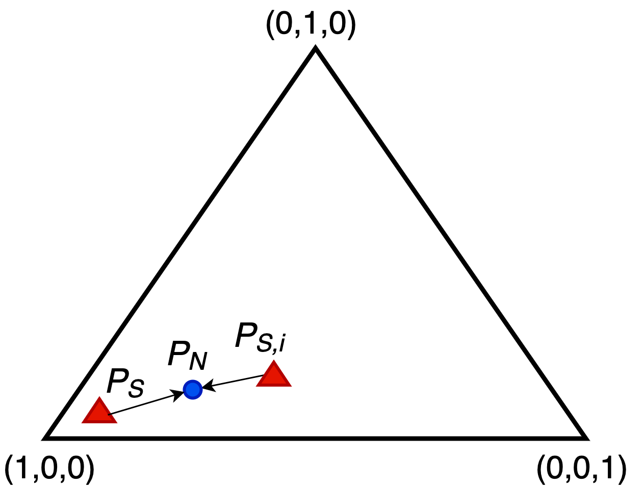
Let us define a function of predictions $P_{S}$ as well as $P_{S,i}$ for all $S$ and $i$ as the distance between $P_{N}$ and $P_{S}$ or $P_{N}$ and $P_{S\cup i}$, denoted as $D(P_{S},P_{N})$ or $D(P_{S,i},P_{N})$, respectively. Let us also introduce the marginal contribution of the $i$-th feature as $D(P_{S},P_{N})-D(P_{S,i},P_{N})$. This is an unusual definition of the marginal contribution can be explained by means of Fig. 1 where two cases of the predicted probability distributions of examples having three features are illustrated in the probabilistic unit simplex with vertices $(1,0,0)$, $(0,1,0)$, $(0,0,1)$. Distributions $P_{S\cup i}$ and $P_{S}$ are depicted by small triangles. Distribution $P_{N}$ is depicted by the small circle.

At first glance, it seems that the contribution of the $i$-th feature should be measured by the distance between points $P_{S}$ and $P_{S,i}$. In particular, if the points coincide, then the distance is zero, and there is no contribution of the considered feature into the prediction or into the class probability distribution. Moreover, Covert et al. [18] proposed to apply the KL divergence $KL\left(P_{S,i}||P_{S}\right)$ to characterize the feature marginal contribution. However, if we look at the right unit simplex in Fig. 1, then we can see that the distance between $P_{S}$ and $P_{S,i}$ is very large. Hence, the marginal contribution of the $i$-th feature should be large. However, after adding the $i$-th feature, we remain to be at the same distance from $P_{N}$. We do not improve our knowledge about the true class or about $P_{N}$ after adding the $i$-th feature to $S$ and computing the corresponding prediction. Note that we do not search for the contribution of the $i$-th feature into the prediction $P_{S}$. We aim to estimate how the $i$-th feature contributes into $P_{N}$. Points $P_{S}$ and $P_{S,i}$ in the right simplex are approximately at the same distance from $P_{N}$, therefore, the difference $D(P_{S},P_{N})-D(P_{S,i},P_{N})$ is close to $0$ though points $P_{S}$ and $P_{S,i}$ are far from each other. The left unit simplex in Fig. 1 shows a different case when $P_{S,i}$ negatively contributes into our knowledge about the class distribution $P_{N}$ because it makes the probability distribution to be more uncertain in comparison with $P_{S}$. This implies that the difference $D(P_{S},P_{N})-D(P_{S,i},P_{N})$ should be negative in this case.

Assuming that $D(P_{S},P_{N})$ is the KL divergence, this distance can be regarded as the information gain achieved if $P_{S}$ would be used instead of $P_{N}$. A similar information gain is achieved if $P_{S,i}$ would be used instead of $P_{N}$. Then we can conclude that the difference $D(P_{S},P_{N})-D(P_{S,i},P_{N})$ can be regarded as the contribution of the $i$-th feature in the change of information gain.

The problem arises when we consider a case illustrated in Fig. 2, where points $P_{S}$ and $P_{S,i}$ are at the same distance from $P_{N}$. However, this case can be also explained in the same way. We do not interpret a final decision about a class of the example. The distribution $P_{0}$ is interpreted here. But this distribution is correctly interpreted because the distribution $P_{S,i}$ does not contribute into $P_{N}$ in comparison with the distribution $P_{S}$. The distribution $P_{S}$ explains the decision $(1,0,0)$ better than $P_{S,i}$, but not than $P_{N}$. Here we meet a situation when interpretation strongly depends on its aim. If its aim is to interpret $P_{N}$ without taking into account the final decision about a class, then we should use the above approach, and contribution of the $i$-th feature in the case illustrated in Fig. 2 is $0$.

Another case is when our aim is to explain the final decision about the predicted class by having predictions in the form of probability distributions. The class can be represented by the probability distribution $P_{0}=(1,0,...,0)$ which is depicted in Fig. 3 by a small square. In this case, we compare distributions $P_{S}$ and $P_{S,i}$ with $P_{0}$, but not with $P_{N}$ because we analyze how the $i$-th feature contributes into change of the decision about the class of the corresponding example, or how this feature contributes into our knowledge about the true class. This is an important difference from the above case when we interpreted $P_{N}$. It can be seen from Fig. 3 that we compute distances $D(P_{S},P_{0})$ and $D(P_{S,i},P_{0})$ instead of $D(P_{S},P_{N})$ and $D(P_{S,i},P_{N})$, respectively. When interpretation of the class is performed, the contribution of the $i$-th feature for the case shown in Fig. 2 is no longer zero. Therefore, we will distinguish the above two cases: interpretation of the class probability distribution and interpretation of the predicted class by using the predicted class probability distribution.

It seems that the distance $D(P_{S},P_{0})$ could be viewed as a measure of uncertainty of the prediction $P_{S}$. However, if we assume that $P_{0}=(1,0,0)$ and $P_{S}=(0,1,0)$, then the distance between distributions is largest, but the distribution $P_{S}$ is certain. In order to consider the uncertainty measure, the distance $D(P_{S},P_{u})$ should be studied in place of $D(P_{S},P_{0})$, where $P_{u}$ is the uniform distribution $(1/C,...,1/C)$. In this case, the distance $D(P_{S},P_{u})$ is a certainty measure of $P_{S}$, because the most uncertain case when $P_{S}=P_{u}$ leads to $D(P_{S},P_{u})=0$.

In sum, the Shapley values are computed now as follows:

Let us study how the introduced distances fulfil basic properties of Shapley values. Their proof directly follows from the representation of the prediction $f(S)$ as $-D(P_{S},P_{N})$ or $-D(P_{S},P_{0})$. Since the condition $f(\emptyset)=0$ may be not valid (the prediction by some predefined feature values), then the efficiency property is rewritten as follows. For the case of the interpretation of the predicted distribution $P_{S}$, the total gain is determined as

Here $P_{\emptyset}$ is the black-box model prediction by replacing all features with some predefined values, for example, with mean values.

Other properties of the Shapley values, including the symmetry, dummy and linearity properties, remain without changes.

We assume that a prediction of the black-box model is imprecise due to due to a small amount of training data, due to our ignorance about a model caused by the lack of observation data. In order to take into account the imprecision, it is proposed to replace precise probability distributions of classes by sets of probability distributions denoted as $\mathcal{P}$, which can be constructed in accordance with one of the well-known imprecise statistical inference models [76].

The imprecision of predictions changes the definition of distances between probability distributions because precise distributions are replaced with sets of probability distributions $\mathcal{P}$. This implies that distances between sets $\mathcal{P}_{1}$ and $\mathcal{P}_{2}$ of distributions should be defined instead of distances between single distributions. We have now a set of distances between all pairs of points such that one point in each pair belongs to set $\mathcal{P}_{1}$, and another point in the pair belongs to set $\mathcal{P}_{2}$. As a results, the set of distances produces an interval with some lower and upper bounds corresponding to the smallest and the largest distances, respectively. The same can be said about pairs of distributions which produce an interval of Shapley values $\phi_{i}$ denoted as $[\phi_{i}^{L},\phi_{i}^{U}]$. This implies that (5) can be rewritten as

where $P$, $R$, $Q$ are probability distributions from subsets $\mathcal{P}(P_{S})$, $\mathcal{P}(P_{S,i})$, $\mathcal{P}(P_{N})$, respectively.

We do not define strongly subsets $\mathcal{P}(P_{S})$, $\mathcal{P}(P_{S,i})$, $\mathcal{P}(P_{N})$ in order to derive general results. We only assume that every subset is convex and is a part of the unit simplex of probabilities. Specific imprecise statistical models producing sets of probability distributions will be considered below.

The next question is how to calculate intervals for Shapley values. A simple way is to separately compute the minimum and the maximum of distances $D$, namely, as follows:

However, obtained intervals of Shapley values may be too wide because we actually consider extreme cases assuming that the distribution $Q\in\mathcal{P}(P_{N})$ may be different in different distances, i.e., in $D(P,Q)$ and $D(R,Q)$. This assumption might be reasonable. Moreover, it would significantly simplify the optimization problems. In order to obtain tighter intervals, we return to (7)-(8). We assume that there exists a single class probability distribution $Q$ from $\mathcal{P}(P_{N})$, which is unknown, but it provides the smallest or the largest value of $D(P,Q)-D(R,Q)$ over all distributions from $\mathcal{P}(P_{N})$. Of course, we relax this condition in other terms of the sum over $S\subseteq N\backslash\{i\}$ because it is extremely difficult to solve the obtained optimization problem under this condition. The same can be said about distributions $P$ and $R$. As a result, we also get wide intervals for Shapley values because, but they will be reduced taking into account intervals for all Shapley values and the efficiency property of the values.

Solutions of optimization problems in (7) and (8) depend on definitions of the distance $D$. Let us return to the efficiency property (6) which is briefly written as $\sum_{k=0}^{m}\phi_{k}=D(P_{\emptyset},P_{N})$. Suppose that we have computed $\phi_{i}^{L}$ and $\phi_{i}^{U}$. Let us denote the lower and upper bounds for $D(P_{\emptyset},P_{N})$ as $D^{L}$ and $D^{U}$, respectively. Then there hold

Hence, the efficiency property of Shapley values can be rewritten by taking into account interval-valued Shapley values as

It follows from (13) that we cannot write a precise version of the efficiency property because we do not know precise distributions $P_{\emptyset}$ and $P_{N}$. Therefore, we use bounds for the total gain, but these bounds can help us to reduce intervals of $\phi_{i}$. Reduced intervals can be obtained by solving the following linear optimization problems:

subject to (13) and $\phi_{k}^{L}\leq\phi_{k}\leq\phi_{k}^{U}$, $k=1,...,m$.

The above optimization problems for all $k$ from $1$ to $m$ allow us to get tighter bounds for Shapley values. It turns out that problems (14) can be explicitly solved. In order to avoid introducing new notations, we assume that all Shapley values are positive. It can be done by subtracting value $\min_{i=1,...,m}\phi_{i}^{L}$ from all variables $\phi_{i}$.

It is interesting to note that the above problem statement is similar to the definitions of reachable probability intervals [22] in the framework of the imprecise probability theory [76]. It can be regarded as an extension of the probabilistic definitions which consider sets of probability distributions as convex subsets of the unit simplex. Moreover, vectors of Shapley values produce a convex set. In contrast to the imprecise probabilities, imprecise Shapley values are not a part of the unit simplex. Transferring definitions of reachable probability intervals to the above problem, we can write that conditions (15) imply that intervals $[\phi_{i}^{L},\phi_{i}^{U}]$ are proper. This implies that the corresponding set of Shapley values is not empty. Moreover, it can be simply proved that bounds $\tilde{\phi}_{k}^{L}$ and $\tilde{\phi}_{k}^{U}$ are reachable. If the reachability condition is not satisfied, then intervals $[\phi_{i}^{L},\phi_{i}^{U}]$ are unnecessarily broad. Moreover, they might be such that some values of the intervals do not correspond to condition (13). Proposition 1 gives a way to compute the reachable intervals of Shapley values. At the same time, it can be extended to a more general case when we would like to find bounds for a linear function $g(\phi_{1},...,\phi_{m})=\sum_{i=1}^{m}$ $a_{i}\phi_{i}=\left\langle\mathbf{a},\mathbf{\phi}\right\rangle$ of imprecise Shapley values. Here $\mathbf{a=(}a_{1}....,a_{m})$ is a vector of known coefficients, $\mathbf{\phi}=(\phi_{1},...,\phi_{m})$. Intervals of $g(\mathbf{\phi}|\mathbf{a})$ are computed by solving the following two linear programming problems (minimization and maximization):

subject to (13) and $\phi_{k}^{L}\leq\phi_{k}\leq\phi_{k}^{U}$, $k=1,...,m$.

The dual optimization problems are

subject to

and

subject to

The above comments can be viewed as a starting point for development of a general theory of imprecise Shapley values. Moreover, Proposition 1 provides a tool for dealing with intervals of Shapley values without assumptions about sets $\mathcal{P}$ of class probability distributions and about the distance $D$ between the sets. Therefore, the next questions are to define imprecise statistical models producing sets $\mathcal{P}$ and the corresponding distances $D$ such that bounds (7)-(8) could be computed in a simple way. In order to answer these questions, we have to select a model producing $\mathcal{P}$ and to select a distance $D$.

There are several imprecise models of probability distributions. One of the interesting models is the linear-vacuous mixture or the imprecise $\varepsilon$-contamination model [76]. It produces a set $\mathcal{P}(\varepsilon,P)$ of probabilities $P^{\ast}=(p_{1}^{\ast},...,p_{C}^{\ast})$ such that $p_{i}^{\ast}=(1-\varepsilon)p_{i}+\varepsilon h_{i}$, where $P=(p_{1},...,p_{C})$ is an elicited probability distribution (in the considered case of SHAP, these distributions are $P_{S}$, $P_{S,i}$, $P_{N}$); $h_{i}\geq 0$ is arbitrary with $h_{1}+...+h_{C}=1$; $0\leq\varepsilon\leq 1$. Parameter $\varepsilon$ controls the size of set $\mathcal{P}(\varepsilon,P)$ and can be defined from size $n$ of the training set. The greater the number of training examples, the less the uncertainty for probability distribution and the less the value of parameter $\varepsilon$. The set $\mathcal{P}(\varepsilon,P)$ is a subset of the unit simplex $S(1,C)$. Moreover, it coincides with the unit simplex when $\varepsilon=1$. According to the model, $\mathcal{P}(\varepsilon,P)$ is the convex set of probabilities with lower bound $(1-\varepsilon)p_{i}$ and upper bound $(1-\varepsilon)p_{i}+\varepsilon$, i.e.,

The convex set has $C$ extreme points, which are all of the same form: the $k$-th element is given by $(1-\varepsilon)p_{i}+\varepsilon$ and the other $T-1$ elements are equal to $(1-\varepsilon)p_{i}$, i.e.,

Fig. 4 illustrates sets $\mathcal{P}(\varepsilon,P_{S})$, $\mathcal{P}(\varepsilon,P_{S,i})$, $\mathcal{P}(\varepsilon,P_{N})$ for precise probability distributions $P_{S}$, $P_{S,i}$, $P_{N}$, respectively, in the form of large triangles around the corresponding distributions. Every distribution belonging to the sets can be a candidate for some “true” distribution which is actually unknown. The imprecise $\varepsilon$-contamination model is equivalent to the imprecise Dirichlet model (IDM) [77] to some extent. The IDM defined by [77] can be viewed as the set of all Dirichlet distributions over $\pi=(\pi_{1},...,\pi_{C})$ with parameters $\alpha=(\alpha_{1},...,\alpha_{C})$ and $s$ such that the vector $\alpha$ belongs to the unit simplex and every $\alpha_{i}$ is the mean of $\pi_{i}$ under the Dirichlet prior. Here $\pi$ is the probability distribution defined on $C$ events, for which the Dirichlet $(s,\alpha)$ prior is defined. For the IDM, the hyperparameter $s$ determines how quickly upper and lower probabilities of events converge as statistical data accumulate. Smaller values of $s$ produce faster convergence and stronger conclusions, whereas large values of $s$ produce more cautious inferences. However, hyperparameter $s$ should not depend on the number of observations. Let $A$ be any non-trivial subset of a sample space, and let $n(A)$ denote the observed number of occurrences of $A$ in the $n$ trials. Then, according to [77], the predictive probability $P(A,s)$ under the Dirichlet posterior distribution is in the following interval

The hyperparameter $s$ of the IDM and parameter $\varepsilon$ of the imprecise $\varepsilon$-contamination model are connected as

Hence, one can see how $\varepsilon$ depends on $n$ by a fixed value of $s$. In particular, $\varepsilon=1$, when $n=0$, and $\varepsilon\rightarrow 0$, when $n\rightarrow\infty$.

In order to apply the SHAP method taking into account the imprecision of the class probability distributions, it is necessary to introduce the distance between probability distributions and to define a way for computing the largest and the smallest distances between all pairs of probability distributions which belong to the small subsets of distributions $\mathcal{P}(\varepsilon,P_{S})$, $\mathcal{P}(\varepsilon,P_{S,i})$, $\mathcal{P}(\varepsilon,P_{N})$.

There are a lot of distance measures between probability distributions. One of the most popular in machine learning measure is the Kullback-Leibler (KL) divergence or relative information [40]:

This measure among other interesting measures, including relative J-divergence [23], relative Arithmetic-Geometric divergence [74], $\chi^{2}$-divergence [56], etc. [33, 74], can be derived using properties of Csiszar’s $f$-divergence measure [19] which is of the form:

where the function $f:(0,\infty)\rightarrow\mathbb{R}$ is convex and normalized, i.e., $f(1)=0$, and it is assumed that $0\cdot f(0/0)=0$ and $0\cdot f(p/0)=0=\lim_{q\rightarrow 0^{+}}qf(p/q)$. For example, functions $f(u)=-\ln u$ and $f(u)=(1-u)^{2}/u$ generate the KL-divergence and the $\chi^{2}$-divergence [53], respectively.

All the aforementioned distance measures lead to very complex optimization problems for computing bounds for distances between subsets of probability distributions. In order to avoid solving the optimization problems, Shapley values can be computed by means of generating a lot of points in subsets $\mathcal{P}(\varepsilon,P_{S})$, $\mathcal{P}(\varepsilon,P_{S,i})$, $\mathcal{P}(\varepsilon,P_{N})$ and computing the smallest and the largest distances or computing the smallest and the largest Shapley values.

There are many algorithms for generating uniformly distributed random points in the unit simplex [55, 65, 66]. One of the well-known and simple algorithms is of the form [66]:

1. 1.

   Generate $k$ independent unit-exponential random variables $Y_{1},...,Y_{k}$ and compute $T_{k}=\sum_{i=1}^{k}Y_{i}$.

2. 2.

   Define $E_{i}=Y_{i}/T_{k}$ and return vector $E=(E_{1},...,E_{k})$ which is uniformly distributed in the unit simplex.

Note that set $\mathcal{P}$ is convex, i.e., it is generated by finitely many linear constraints. This implies that it is totally defined by its extreme points or vertices denoted $\mathcal{E}(\mathcal{P})$. Suppose that we have a set of $r$ extreme points $Q_{k}=(q_{1}^{(k)},...,q_{C}^{(k)})$ of the set $\mathcal{P}$, i.e., $q_{k}\in\mathcal{E}(\mathcal{P})$, $k=1,...,r$. In the case of the imprecise $\varepsilon$-contamination model, there holds $r=C.$ Then every probability distribution $P=(p_{1},...,p_{C})$ from $\mathcal{P}$ can be represented as the linear combination of the extreme points

Here $\lambda=(\lambda_{1},...,\lambda_{r})$ is a vector of weights such that $\lambda_{1}+...+\lambda_{r}=1$.

If to uniformly generate vectors $\lambda$ from the unit simplex by using one of the known algorithms of generation, then random points $P$ from the set $\mathcal{P}$ can be obtained. Extreme points of set $\mathcal{P}$ for the imprecise $\varepsilon$-contamination model are given in (19).

From all generated points in $\mathcal{P}(\varepsilon,P_{S})$, $\mathcal{P}(\varepsilon,P_{S,i})$, $\mathcal{P}(\varepsilon,P_{N})$, we select three corresponding points, say, $P_{1}\in\mathcal{P}(\varepsilon,P_{S})$, $R_{1}\in\mathcal{P}(\varepsilon,P_{S,i})$, $Q_{1}\in\mathcal{P}(\varepsilon,P_{N})$ such that the difference $D(P,Q)-D(R,Q)$ of distances achieves its minimum. These points contribute into the lower Shapley value $\phi_{i}^{L}$. In the same way, three points $P_{2}$, $R_{2}$, $Q_{2}$ are selected from the same sets, respectively, such that the difference $D(P,Q)-D(R,Q)$ achieves its maximum. These points contribute into the upper Shapley value $\phi_{i}^{U}$. This procedure is repeated for all Shapley values $\phi_{i}$, $i=1,...,m$.

The main advantage of the above generation approach for computing the lower and upper Shapley values is that an arbitrary distance between probability distributions can be used for implementing the approach, for example, the KL divergence or the $\chi^{2}$-divergence. There are no restrictions for selecting distances. Moreover, intervals for Shapley values can be also directly computed. Of course, this approach may be extremely complex especially when training examples have a high dimension and parameter $\varepsilon$ of the imprecise $\varepsilon$-contamination model is rather large (the imprecise model produces large sets $\mathcal{P}(\varepsilon,\cdot)$). Moreover, it is difficult to control the accuracy of the obtained Shapley values because there is a chance that the selected points $P_{1}$, $R_{1}$, $Q_{1}$ and $P_{2}$, $R_{2}$, $Q_{2}$ may be not optimal, i.e., the corresponding differences $D(P,Q)-D(R,Q)$ do not achieve the minimum and the maximum. In order to overcome this difficulty, another approach is proposed, which is based on applying the Kolmogorov-Smirnov distance leading to a set of very simple linear programming problems.

References

- [1] K. Aas, M. Jullum, and A. Loland. Explaining individual predictions when features are dependent: More accurate approximations to Shapley values. arXiv:1903.10464, Mar 2019.
- [2] J. Abellan, R.M. Baker, F.P.A. Coolen, R.J. Crossman, and A.R. Masegosa. Classification with decision trees from a nonparametric predictive inference perspective. Computational Statistics and Data Analysis, 71:789–802, 2014.
- [3] J. Abellan, C.J. Mantas, and J.G. Castellano. A random forest approach using imprecise probabilities. Knowledge-Based Systems, 134:72–84, 2017.
- [4] J. Abellan, C.J. Mantas, J.G. Castellano, and S. Moral-Garcia. Increasing diversity in random forest learning algorithm via imprecise probabilities. Expert Systems With Applications, 97:228–243, 2018.
- [5] J. Abellan and S. Moral. Building classification trees using th building classification trees using the total uncertainty criterion. International Journal of Intelligent Systems, 18(12):1215–1225, 2003.
- [6] A. Adadi and M. Berrada. Peeking inside the black-box: A survey on explainable artificial intelligence (XAI). IEEE Access, 6:52138–52160, 2018.
- [7] R. Agarwal, N. Frosst, X. Zhang, R. Caruana, and G.E. Hinton. Neural additive models: Interpretable machine learning with neural nets. arXiv:2004.13912, April 2020.
- [8] L. Antwarg, R.M. Miller, B. Shapira, and L. Rokach. Explaining anomalies detected by autoencoders using SHAP. arXiv:1903.02407v2, June 2020.
- [9] A.B. Arrieta, N. Diaz-Rodriguez, J. Del Ser, A. Bennetot, S. Tabik, A. Barbado, S. Garcia, S. Gil-Lopez, D. Molina, R. Benjamins, R. Chatila, and F. Herrera. Explainable artificial intelligence (XAI): Concepts, taxonomies, opportunities and challenges toward responsible AI. arXiv:1910.10045, October 2019.
- [10] V. Belle and I. Papantonis. Principles and practice of explainable machine learning. arXiv:2009.11698, September 2020.
- [11] V. Van Belle, K. Pelckmans, S. Van Huffel, and J.A. Suykens. Support vector methods for survival analysis: a comparison between ranking and regression approaches. Artificial intelligence in medicine, 53(2):107–118, 2011.
- [12] J. Bento, P. Saleiro, A.F. Cruz, M.A.T. Figueiredo, and P. Bizarro. TimeSHAP: Explaining recurrent models through sequence perturbations. arXiv:2012.00073, November 2020.
- [13] P. Bonissone, J.M. Cadenas, M.C. Garrido, and R.A. Diaz-Valladares. A fuzzy random forest. International Journal of Approximate Reasoning, 51:729–747, 2010.
- [14] D. Bowen and L. Ungar. Generalized SHAP: Generating multiple types of explanations in machine learning. arXiv:2006.07155v2, June 2020.
- [15] D.V. Carvalho, E.M. Pereira, and J.S. Cardoso. Machine learning interpretability: A survey on methods and metrics. Electronics, 8(832):1–34, 2019.
- [16] C.-H. Chang, S. Tan, B. Lengerich, A. Goldenberg, and R. Caruana. How interpretable and trustworthy are gams? arXiv:2006.06466, June 2020.
- [17] I.C. Covert, S. Lundberg, and S.-I. Lee. Explaining by removing: A unified framework for model explanation. arXiv:2011.14878, November 2020.
- [18] I.C. Covert, S. Lundberg, and S.-I. Lee. Understanding global feature contributions with additive importance measures. arXiv:2004.00668v2, October 2020.
- [19] I. Csiszar. Information type measures of differences of probability distribution and indirect observations. Studia Scientiarum Mathematicarum Hungarica, 2(:299–318, 1967.
- [20] A. Das and P. Rad. Opportunities and challenges in explainableartificial intelligence (XAI): A survey. arXiv:2006.11371v2, June 2020.
- [21] G.V. den Broeck, A. Lykov, M. Schleich, and D. Suciu. On the tractability of SHAP explanations. arXiv:2009.08634v2, January 2021.
- [22] S. Destercke and V. Antoine. Combining imprecise probability masses with maximal coherent subsets: Application to ensemble classification. In Synergies of Soft Computing and Statistics for Intelligent Data Analysis, pages 27–35. Springer, Berlin, Heidelberg, 2013.
- [23] S.S. Dragomir, V. Gluscevic, and C.E.M. Pearce. Approximations for the csiszar’s fdivergence via mid point inequalities. In Inequality Theory and Applications, pages 139–154. Nova Science Publishers Inc., Huntington, New York, 2001.
- [24] D. Faraggi and R. Simon. A neural network model for survival data. Statistics in medicine, 14(1):73–82, 1995.
- [25] C. Frye, D. de Mijolla, L. Cowton, M. Stanley, and I. Feige. Shapley-based explainability on the data manifold. arXiv:2006.01272, June 2020.
- [26] D. Garreau and D. Mardaoui. What does LIME really see in images? arXiv:2102.06307, February 2021.
- [27] D. Garreau and U. von Luxburg. Explaining the explainer: A first theoretical analysis of LIME. arXiv:2001.03447, January 2020.
- [28] D. Garreau and U. von Luxburg. Looking deeper into tabular LIME. arXiv:2008.11092, August 2020.
- [29] R. Guidotti, A. Monreale, S. Ruggieri, F. Turini, F. Giannotti, and D. Pedreschi. A survey of methods for explaining black box models. ACM computing surveys, 51(5):93, 2019.
- [30] T. Hastie and R. Tibshirani. Generalized additive models, volume 43. CRC press, 1990.
- [31] Q. Huang, M. Yamada, Y. Tian, D. Singh, D. Yin, and Y. Chang. GraphLIME: Local interpretable model explanations for graph neural networks. arXiv:2001.06216, January 2020.
- [32] N.A. Ibrahim, A. Kudus, I. Daud, and M.R. Abu Bakar. Decision tree for competing risks survival probability in breast cancer study. International Journal Of Biological and Medical Research, 3(1):25–29, 2008.
- [33] K.C. Jain and P. Chhabra. Bounds on nonsymmetric divergence measure in terms ofother symmetric and nonsymmetric divergence measures. International Scholarly Research Notices, 2014(Article ID 820375):1–9, 2014.
- [34] N.L. Johnson and F. Leone. Statistics and experimental design in engineering and the physical sciences, volume 1. Wiley, New York, 1964.
- [35] A. Jung. Explainable empirical risk minimization. arXiv:2009.01492, September 2020.
- [36] J.L. Katzman, U. Shaham, A. Cloninger, J. Bates, T. Jiang, and Y. Kluger. Deepsurv: Personalized treatment recommender system using a Cox proportional hazards deep neural network. BMC medical research methodology, 18(24):1–12, 2018.
- [37] A.V. Konstantinov and L.V. Utkin. Interpretable machine learning with an ensemble of gradient boosting machines. arXiv:2010.07388, October 2020.
- [38] M.S. Kovalev and L.V. Utkin. A robust algorithm for explaining unreliable machine learning survival models using the Kolmogorov-Smirnov bounds. Neural Networks, 132:1–18, 2020.
- [39] M.S. Kovalev, L.V. Utkin, and E.M. Kasimov. SurvLIME: A method for explaining machine learning survival models. Knowledge-Based Systems, 203:106164, 2020.
- [40] S. Kullback and R.A. Leibler. On information and sufficiency. Annals of Mathematical Statistics, 22:9–86, 1951.
- [41] Y. Liang, S. Li, C. Yan, M. Li, and C. Jiang. Explaining the black-box model: A survey of local interpretation methods for deep neural networks. Neurocomputing, 419:168–182, 2021.
- [42] M. Lichman. UCI machine learning repository, 2013.
- [43] Y. Lou, R. Caruana, and J. Gehrke. Intelligible models for classification and regression. In Proceedings of the 18th ACM SIGKDD International Conference on Knowledge Discovery and Data Mining, pages 150–158. ACM, August 2012.
- [44] S.M. Lundberg and S.-I. Lee. A unified approach to interpreting model predictions. In Advances in Neural Information Processing Systems, pages 4765–4774, 2017.
- [45] S. Mangalathu, S.-H. Hwang, and J.-S. Jeon. Failure mode and effects analysis of RC members based on machinelearning-based SHapley Additive exPlanations (SHAP) approach. Engineering Structures, 219:110927 (1–10), 2020.
- [46] C.J. Mantas and J. Abellan. Analysis and extension of decision trees based on imprecise probabilities: Application on noisy data. Expert Systems with Applications, 41(5):2514–2525, 2014.
- [47] R. Marcinkevics and J.E. Vogt. Interpretability and explainability: A machine learning zoo mini-tour. arXiv:2012.01805, December 2020.
- [48] P.-A. Matt. Uses and computation of imprecise probabilities from statistical data and expert arguments. International Journal of Approximate Reasoning, 81:63–86, 2017.
- [49] C. Molnar. Interpretable Machine Learning: A Guide for Making Black Box Models Explainable. Published online, https://christophm.github.io/interpretable-ml-book/, 2019.
- [50] I. Montes, E. Miranda, and S. Destercke. Unifying neighbourhood and distortion models: part ii – new models and synthesis. International Journal of General Systems, 49(6):636–674, 2020.
- [51] S. Moral. Learning with imprecise probabilities as model selection and averaging. International Journal of Approximate Reasoning, 109:111–124, 2019.
- [52] S. Moral-Garcia, C.J. Mantas, J.G. Castellano, M.D. Benitez, and J. Abellan. Bagging of credal decision trees for imprecise classification. Expert Systems with Applications, 141(Article 112944):1–9, 2020.
- [53] F. Nielsen and R. Nock. On the chi square and higher-order chi distances for approximating f-divergences. IEEE Signal Processing Letters, 21(1):10–13, 2014.
- [54] H. Nori, S. Jenkins, P. Koch, and R. Caruana. InterpretML: A unified framework for machine learning interpretability. arXiv:1909.09223, September 2019.
- [55] S. Onn and I. Weissman. Generating uniform random vectors over a simplexwith implications to the volume of a certain polytopeand to multivariate extremes. Annals of Operations Research, 189:331–342, 2011.
- [56] K. Pearson. On the criterion that a given system of eviations from the probable in the case of correlated system of variables is such that it can be reasonable supposed to have arisen from random sampling. Philosophical Magazine, 50:157–172, 1900.
- [57] V. Petsiuk, A. Das, and K. Saenko. RISE: Randomized input sampling for explanation of black-box models. arXiv:1806.07421, June 2018.
- [58] J. Rabold, H. Deininger, M. Siebers, and U. Schmid. Enriching visual with verbal explanations for relational concepts: Combining LIME with Aleph. arXiv:1910.01837v1, October 2019.
- [59] A. Redelmeier, M. Jullum, and K. Aas. Explaining predictive models with mixed features using shapley values and conditional inference trees. In Machine Learning and Knowledge Extraction. CD-MAKE 2020, volume 12279 of Lecture Notes in Computer Science, pages 117–137, Cham, 2020. Springer.
- [60] M.T. Ribeiro, S. Singh, and C. Guestrin. “Why should I trust You?” Explaining the predictions of any classifier. arXiv:1602.04938v3, Aug 2016.
- [61] M.T. Ribeiro, S. Singh, and C. Guestrin. Anchors: High-precision model-agnostic explanations. In AAAI Conference on Artificial Intelligence, pages 1527–1535, 2018.
- [62] C.P. Robert. The Bayesian Choice. Springer, New York, 1994.
- [63] R. Rodriguez-Perez and J. Bajorath. Interpretation of machine learning models using shapley values: application to compound potency and multi-target activity predictions. Journal of Computer-Aided Molecular Design, 34:1013–1026, 2020.
- [64] B. Rozemberczki and R. Sarkar. The shapley value of classifiers in ensemble games. arXiv:2101.02153, January 2021.
- [65] R.Y. Rubinstein and D.P. Kroese. Simulation and the Monte Carlo method, 2nd Edition. Wiley, New Jersey, 2008.
- [66] R.Y. Rubinstein and B. Melamed. Modern simulation and modeling. Wiley, New York, 1998.
- [67] C. Rudin. Stop explaining black box machine learning models for high stakes decisions and use interpretable models instead. Nature Machine Intelligence, 1:206–215, 2019.
- [68] C. Rudin, C. Chen, Z. Chen, H. Huang, L. Semenova, and C. Zhong. Interpretable machine learning: Fundamental principles and 10 grand challenges. arXiv:2103.11251, March 2021.
- [69] R. Senge, S. Bosner, K. Dembczynski, J. Haasenritter, O. Hirsch, N. Donner-Banzhoff, and E. Hüllermeier. Reliable classification: Learning classifiers that distinguish aleatoric and epistemic uncertainty. Information Sciences, 255:16–29, 2014.
- [70] S.M. Shankaranarayana and D. Runje. ALIME: Autoencoder based approach for local interpretability. arXiv:1909.02437, Sep 2019.
- [71] L.S. Shapley. A value for n-person games. In Contributions to the Theory of Games, volume II of Annals of Mathematics Studies 28, pages 307–317. Princeton University Press, Princeton, 1953.
- [72] E. Strumbelj and I. Kononenko. An efficient explanation of individual classifications using game theory. Journal of Machine Learning Research, 11:1–18, 2010.
- [73] N. Takeishi. Shapley values of reconstruction errors of PCA for explaining anomaly detection. arXiv:1909.03495, September 2019.
- [74] I.J. Taneja and P. Kumar. Generalized non-symmetric divergence measures and inequaities. Journal of Interdisciplinary Mathematics, 9(3):581–599, 2006.
- [75] L.V. Utkin and A.V. Konstantinov. Ensembles of random SHAPs. arXiv:2103.03302, March 2021.
- [76] P. Walley. Statistical Reasoning with Imprecise Probabilities. Chapman and Hall, London, 1991.
- [77] P. Walley. Inferences from multinomial data: Learning about a bag of marbles. Journal of the Royal Statistical Society, Series B, 58:3–57, 1996. with discussion.
- [78] M.N. Wright, T. Dankowski, and A. Ziegler. Unbiased split variable selection for random survival forests using maximally selected rank statistics. Statistics in Medicine, 36(8):1272–1284, 2017.
- [79] N. Xie, G. Ras, M. van Gerven, and D. Doran. Explainable deep learning: A field guide for the uninitiated. arXiv:2004.14545, April 2020.
- [80] J. Yu, Z. Lin, J. Yang, X. Shen, X. Lu, and T.S. Huang. Generative image inpainting with contextual attention. In Proceedings of the IEEE Conference on Computer Vision and Pattern Recognition, pages 5505–5514, 2018.
- [81] H. Yuan, H. Yu, J. Wang, K. Li, and S. Ji. On explainability of graph neural networks via subgraph explorations. arXiv:2102.05152, February 2020.
- [82] E. Zablocki, H. Ben-Younes, P. Perez, and M. Cord. Explainability of vision-based autonomous driving systems: Review and challenges. arXiv:2101.05307, January 2021.
- [83] M.D. Zeiler and R. Fergus. Visualizing and understanding convolutional networks. In ECCV 2014, volume 8689 of LNCS, pages 818–833, Cham, 2014. Springer.
- [84] X. Zhang, S. Tan, P. Koch, Y. Lou, U. Chajewska, and R. Caruana. Axiomatic interpretability for multiclass additive models. In In Proceedings of the 25th ACM SIGKDD International Conference on Knowledge Discovery & Data Mining, pages 226–234. ACM, 2019.
- [85] Y. Zhang, P. Tino, A. Leonardis, and K. Tang. A survey on neural network interpretability. arXiv:2012.14261, December 2020.