Constraints on bimetric gravity from Big Bang nucleosynthesis

Since the Universe is currently expanding, even accelerating Riess et al. 1998; Perlmutter et al. 1999, tracing the expansion history backwards in time, the Universe must have been in a very hot and dense initial state. These conditions are appropriate for nuclear reactions to take place, leading to the production of the light elements, including D (deuterium) and ${}^{4}\mathrm{He}$, referred to as Big Bang nucleosynthesis (BBN). The resulting abundances of these light elements depend on the conditions at this period, for example on the expansion rate of the Universe and the number of neutrino species. Hence, given the observed abundances of light elements, BBN can be used to test non-standard cosmologies.

The cosmological concordance model is based on general relativity (GR) and the standard model of particle physics and has been very successful in accounting for (and predicting) cosmological observations, including the abundances of the light elements Alpher et al. 1948. However, to fit observations, one introduces two elusive ingredients, the cosmological constant ($\Lambda$) and a cold dark matter (CDM) particle, constituting the $\Lambda$CDM model. The cosmological constant must be extremely fine-tuned in order to almost exactly cancel the quantum contributions to the vacuum energy. The CDM particle makes up the main part of the matter content of the Universe, yet there is no direct detection of this particle(s). Moreover, with increasingly precise observations, a tension has appeared recently between the value of the Hubble constant (i.e., the present-day expansion rate) as inferred from small and large distance measurements, see for example Verde et al. 2019. These issues, together with the problem (or impossibility) of quantizing GR, suggest that Einstein’s theory of general relativity is not the ultimate theory for gravity.

Bimetric gravity is a natural extension of general relativity, introducing a massive spin-2 field in addition to the massless spin-2 field (identified with the metric in GR) Hassan and Rosen 2012a; Hassan et al. 2013. Accordingly, there are two gravitons, one massive and one massless. The presence of the massless graviton allows gravitational wave observations to be satisfied without severely restricting the parameter space of the theory Max et al. 2017, as opposed to many other modified gravity models. Bimetric gravity is also compatible with cosmological observations like the cosmic microwave background (CMB), type Ia supernovae (SNIa), and baryon acoustic oscillations (BAO) von Strauss et al. 2012; Akrami et al. 2013; Koennig et al. 2014a; Lüben et al. 2020; Dhawan et al. 2017; Lindner et al. 2020; Caravano et al. 2021; Högås and Mörtsell 2021a and it exhibits a screening mechanism that restores general relativity results on solar-system scales Sjors and Mortsell 2013; Enander and Mörtsell 2013; Babichev and Crisostomi 2013; Enander and Mortsell 2015; Platscher et al. 2018; Lüben et al. 2020a. Among the interesting properties of the theory are:

• •

  Cosmologies where the accelerated expansion is due to the interaction between the massless and massive spin-2 fields. No cosmological constant is needed Volkov 2012a; von Strauss et al. 2012; Comelli et al. 2012a; Volkov 2012b; Volkov 2012c; Akrami et al. 2013; Volkov 2013; Koennig et al. 2014a; Högås and Mörtsell 2021b; Högås and Mörtsell 2021a.
  

• •

  In a certain parameter range, the massive graviton can function as a dark matter particle Aoki and Mukohyama 2016; Babichev et al. 2016a; Babichev et al. 2016b. Part of the need of dark matter in local environments can also be reduced with a scale-dependent gravitational coupling “constant” Enander and Mortsell 2015; Platscher et al. 2018; Högås and Mörtsell 2021b.
  

• •

  The increased spectrum of cosmological solutions opens up the possibility to ease the Hubble tension. Preliminary studies suggest that the tension can be eased at least to a small degree Mörtsell and Dhawan 2018; Högås and Mörtsell 2021a.

Challenges to the theory include the appearance of a gradient instability at the linear perturbative level around (homogeneous and isotropic) cosmological backgrounds Comelli et al. 2012b; Khosravi et al. 2012; Berg et al. 2012; Sakakihara et al. 2013; Könnig and Amendola 2014; Comelli et al. 2014; De Felice et al. 2014; Solomon et al. 2014; Koennig et al. 2014b; Lagos and Ferreira 2014; Könnig 2015; Aoki et al. 2015; Mortsell and Enander 2015; Akrami et al. 2015; Högås et al. 2020; Lüben et al. 2020b. This means that structure formation cannot be analyzed using linear perturbation theory, instead it is necessary to solve the full non-linear equations of motion Aoki et al. 2015; Mortsell and Enander 2015; Högås et al. 2020, requiring a stable (well-posed) form of the equations of motion. Partial progress has been made in that direction Kocic 2021; Kocic 2019; Kocic et al. 2019a; Torsello et al. 2020; Kocic et al. 2019b; Torsello 2019; Torsello 2020; Kocic et al. 2020, but a well-posed form of the equations of motion is still unknown.

The bimetric action (Hassan–Rosen action) is,

where $g$ and $f$ denote the determinants of the two metrics (spin-2 fields) $g_{\mu\nu}$ and $f_{\mu\nu}$, $R$ is the Ricci scalar of $g_{\mu\nu}$ and $\widetilde{R}$ the Ricci scalar of $f_{\mu\nu}$, $\kappa_{g}$ and $\kappa_{f}$ are the Einstein gravitational constants of the two metrics¹¹ 1 $\kappa_{g}=8\pi G/c^{4}$ in SI-units., the $\beta$-parameters are five, free, constant parameters with dimension of curvature ($1/\mathsf{L}^{2}$), $e_{n}(S)$ are the elementary symmetric polynomials of the square root $S^{\mu}{}_{\nu}$, defined by $S^{\mu}{}_{\rho}S^{\rho}{}_{\nu}=g^{\mu\rho}f_{\rho\nu}$, and $\mathcal{L}_{m}$ is the matter Lagrangian. The action is constructed to avoid the Boulware–Deser ghost plaguing generic theories of massive gravity Boulware and Deser 1972; Hassan and Rosen 2012a; Hassan and Rosen 2012b; Hassan and Lundkvist 2018.

Traditionally, the $\beta$-parameters are used as the free parameters of bimetric gravity. However, the Hassan–Rosen action is invariant under the rescaling $(f_{\mu\nu},\kappa_{f},\beta_{n})\to(\omega f_{\mu\nu},\omega\kappa_{f},\omega^{-n/2}\beta_{n})$ with $\omega=\mathrm{const}$. Thus, the $\beta$-parameters are not observables and cannot be constrained by observations (without first having to specify a choice of scaling). This problem is circumvented by introducing the rescaling-invariant (dimensionless) parameters,

where $H_{0}$ is the Hubble constant and $c$ is the conformal factor between the two metrics in the asymptotic future when the metrics are proportional $f_{\mu\nu}=c^{2}g_{\mu\nu}$ (see below and Ref. Högås and Mörtsell 2021b). With the $B$-parameters, we can define the physical parameters $\Theta=(\theta,m_{\mathrm{FP}},\Omega_{\Lambda},\alpha,\beta)$ Lüben et al. 2020b; Lüben et al. 2020; Högås and Mörtsell 2021b, see Appendix A for details. These parameters have immediate physical interpretations; $\theta$ is the mixing angle between the massive and massless gravitons. When $\theta=0$, the physical metric $g_{\mu\nu}$ is aligned with the massless graviton and the theory reduces to GR, whereas if $\theta=90^{\circ}$, the physical metric is aligned with the massive graviton and the theory reduces to de Rham–Gabadadze–Tolley (dRGT) massive gravity with a fixed reference metric de Rham and Gabadadze 2010; de Rham et al. 2011; Hassan and Rosen 2012c; Hassan et al. 2012; de Rham 2014. $m_{\mathrm{FP}}$ is the mass of the (massive) graviton measured in units of $H_{0}\sim 10^{-33}\,\mathrm{eV}/c^{2}$, $\Omega_{\Lambda}$ is the effective cosmological constant that bimetric cosmology approaches in the asymptotic future, and $\alpha$ and $\beta$ are parameters which (among other things) determine the screening mechanism, see Ref. Högås and Mörtsell 2021b for details. There is a one-to-one relation between the $B$-parameters and the physical parameters, so due to their immediate physical interpretation, we choose to parameterize the theory in terms of the latter.

In bimetric gravity, the Friedmann equation is modified by the addition of a dynamical energy density giving a dark energy contribution,

The equation of state parameter $w_{\mathrm{DE}}(z)$ depends on time (redshift), with the functional form depending on the physical parameters, see Ref. Högås and Mörtsell 2021b for an explicit expression and Fig. 1 for some examples. Here, $\Omega_{x}$ is the present-day energy density of species $x$, measured in terms of the critical density today,

The dark energy density increases with time and contributes to the accelerated expansion of the Universe (hence the subscript “DE” for dark energy).

Bimetric cosmology is characterized by a late-universe phase, where the dark energy acts as a cosmological constant with energy density $\Omega_{\Lambda}$. Thus, the Universe approaches a de Sitter phase in the asymptotic future, as in the $\Lambda$CDM model. In the early universe, $\rho_{\mathrm{DE}}$ becomes subdominant and the expansion mimics $\Lambda$CDM again. In the intermediate region, $\rho_{\mathrm{DE}}$ is dynamical. In this phase, there is a wide range of different expansion histories, depending on the physical parameters Högås and Mörtsell 2021b. The redshift at which this dynamical transition takes place will be referred to as $z_{t}$ and its value is set by the parameters $(m_{\mathrm{FP}},\alpha,\beta)$, such that larger values push the transition backwards in time (i.e., to higher redshifts). The redshift at matter-radiation equality is denoted $z_{\mathrm{eq}}$.

If $0\ll z_{t}\ll z_{\mathrm{eq}}$ (i.e., $m_{\mathrm{FP}}$, $\alpha$, and $\beta$ not very large), the expansion rate is increased in the region $z_{t}\lesssim z\ll z_{\mathrm{eq}}$ reaching a maximum value of,

see Ref. Högås and Mörtsell 2021b. Hence, $S-1$ is the relative difference between the bimetric model and the GR ($\Lambda$CDM) model. Here, we have set the Hubble constant of the two models to be equal. When $z\gtrsim z_{\mathrm{eq}}$, the expansion follows the $\Lambda$CDM model again, implying that there is no modification of the expansion rate at BBN for these values of the parameters.

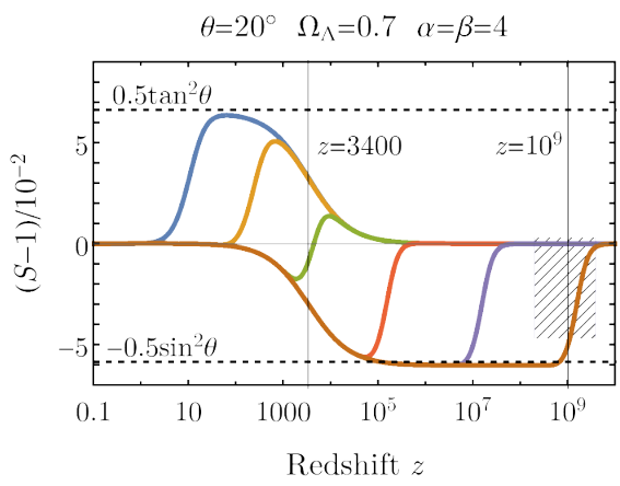
On the other hand, if the transition takes place in the radiation-dominated era $z_{t}\gg z_{\mathrm{eq}}$ (i.e., if $m_{\mathrm{FP}}$, $\alpha$ or $\beta\gg 1$), the bimetric dark energy mimics a relativistic species with negative energy density in the redshift range $z_{\mathrm{eq}}\lesssim z\lesssim z_{t}$. Hence, in this regime there is a decreased expansion rate, reaching a minimum value of,

See Fig. 2 for some examples. When $z\gtrsim z_{t}$, the dark energy is subdominant and the expansion history follows the $\Lambda$CDM model again. For large enough values of $m_{\mathrm{FP}}$, $\alpha$, or $\beta$, the period of decreased expansion rate extends to the range relevant for BBN (i.e., $z\sim 10^{9}$), thus setting an upper limit on $\theta$, assuming that $S_{\mathrm{BBN}}\simeq 1$.

The baryon-to-photon ratio is parameterized by,

where $n_{x}$ denotes the number density of species $x$. After electron-positron annihilation, the number of baryons and photons in a comoving volume is constant. Hence, the right-hand side of (7) can be evaluated at present day or at BBN, with the same result. The D abundance can be used to determine $\eta_{10}$ Kneller and Steigman 2004, with the result Cyburt et al. 2016; Fields et al. 2020,

This is consistent with the values derived from CMB data from the Planck satellite Cyburt et al. 2016; Fields et al. 2020. Whereas D works as a baryometer, ${}^{4}\mathrm{He}$ works as a chronometer, restricting the expansion rate, $S$, at BBN. The ${}^{4}\mathrm{He}$ abundance can be approximated by the linear relation Kneller and Steigman 2004; Steigman 2007,

where the second term on the right-hand side is the numerical error due to the approximation. Here, we assume standard model particle physics with bimetric gravity only modifying the background expansion, $S\neq 1$.

In more recent works, the theoretical model prediction of $Y_{p}$ is typically parameterized in terms of an effective additional number of neutrino species, $\Delta N_{\nu}$, rather than in terms of $S$, see for example Pitrou et al. 2018; Pitrou et al. 2021; Cyburt et al. 2016; Fields et al. 2020; Yeh et al. 2021; Pisanti et al. 2021. In these works, higher-order corrections to the linear model (9) are also included. A greater number of neutrino species leads to an increased expansion rate and vice versa for a decreasing number. The modification is achieved by making the replacement $\rho_{r}\to\rho_{r}^{\prime}=\rho_{r}+\Delta N_{\nu}\rho_{\nu}$, which leads to $S^{2}=1+\Delta N_{\nu}\rho_{\nu}/\rho_{r}$. Before electron-positron annihilation, it reads $S^{2}=1+21\Delta N_{\nu}/43$ which can be used to translate between $S\leftrightarrow\Delta N_{\nu}$.²² 2 Note however, that $S$ is the more fundamental parameter as it allows for a general form of the modified expansion rate. For our purposes however, the linear model (9) is sufficient. For example, in the range $S=0.978\pm 0.025$ (cf. (11)), the numerical error of the linear model is only $0.5\,\%$ compared with the expression including corrections up to third order in $\Delta N_{\nu}$ Pitrou et al. 2018.

From astrophysical observations, the ${}^{4}\mathrm{He}$ abundance is determined to Aver et al. 2015,

consistent with the results of Refs. Peimbert et al. 2016; Fernández et al. 2018; Fields et al. 2020. Within GR, $S=1$ and the predicted abundance according to (9) is $Y_{p}^{\mathrm{GR}}=0.2484\pm(0.0006)_{\mathrm{num}}$, slightly higher than, but consistent with, the observed value (10). A slower expansion rate ($S<1$) gives more time for neutrons to transform into protons and the lower neutron abundance results in a decrease of the ${}^{4}\mathrm{He}$ abundance ($Y_{p}$). With (9)-(10) and using the value (8), we derive the following constraint on the expansion rate at BBN,

which can be used to constrain the bimetric parameter space. For models where $H/H_{\mathrm{GR}}$ is varying during BBN (e.g. the $m_{\mathrm{FP}}=10^{16}$ model in Fig. 2), $S$ is set to the average value of $H/H_{\mathrm{GR}}$ within the redshift range $0.2\times 10^{9}\lesssim z\lesssim 3.7\times 10^{9}$. Using (6), we predict the constraint $\theta\lesssim 18^{\circ}$ on the mixing angle in the region where $m_{\mathrm{FP}}$, $\alpha$, or $\beta$ are large enough for $\rho_{\mathrm{DE}}$ to become subdominant at redshifts greater than BBN ($z\sim 10^{9}$).

When scanning the parameter space, the present-day matter density ($\Omega_{m}$) is fixed by the physical parameters (see Ref. Högås and Mörtsell 2021b) and the present-day radiation density is set by the current CMB temperature and the neutrino physics, which we assume to be standard, yielding $\Omega_{r}\simeq 9\times 10^{-5}$. Note however that there is a degree of degeneracy in $Y_{p}$ between the number of neutrino species and a modified expansion history, as discussed above.

The light element abundances are sensitive to the expansion rate in the range $0.2\times 10^{9}\lesssim z\lesssim 3.7\times 10^{9}$, corresponding to temperatures $0.06\,\mathrm{MeV}\lesssim T\lesssim 1\,\mathrm{MeV}$. We exclude regions in parameter space which violate the observational constraint (11) in this redshift range. The result is shown in Fig. 3. It is evident that the GR limit ($\theta\to 0$) is included in the allowed parameter range, but the bimetric model gives a slightly better fit. For example, in the range $m_{\mathrm{FP}}\gtrsim 10^{-16}\,\mathrm{eV}/c^{2}$, the best fit is $\theta\simeq 12^{\circ}$, giving a slightly slower expansion rate at BBN compared with GR. When $m_{\mathrm{FP}}\gtrsim 10^{-16}\,\mathrm{eV}/c^{2}$ or $\alpha\gtrsim 10^{34}$ or $\beta\gtrsim 10^{36}$, the mixing angle must satisfy $\theta\lesssim 18^{\circ}$, in accordance with our prediction.

In Fig. 4, we compile the BBN results together with constraints from other observational probes. The constraints from gravitational waves (GWs) are from LIGO/Virgo observations of GWs from binary merger systems (neutron star-neutron star or black hole-black hole). The interaction between the massless and massive waves changes the waveform compared with GR. Demanding the waveform to be within observational bounds excludes a graviton mass $10^{11}\lesssim m_{\mathrm{FP}}\lesssim 10^{12}$ in the mixing angle range $17^{\circ}\lesssim\theta\lesssim 73^{\circ}$ (cf. Max et al. 2017). The event GW170817 came with an electromagnetic counterpart Abbott et al. 2017a; Abbott et al. 2017b, constraining the propagation speed of gravitational waves to be within one part in $10^{15}$ of the speed of light Abbott et al. 2017c. The observation excludes $m_{\mathrm{FP}}\gtrsim 10^{12}$ if $\theta\gtrsim 70^{\circ}$. The electromagnetic signal also allows to identify the host galaxy, to which a GW-independent distance measure can be calculated, using the redshift of the galaxy and assuming a cosmological model (in this case $\Lambda$CDM). The distance can also be estimated from the gravitational wave detection. A significant mixing between the massless and massive graviton implies a modified distance. To be compatible with the GW-independent value, we exclude $15^{\circ}\lesssim\theta\lesssim 75^{\circ}$ if $m_{\mathrm{FP}}\gtrsim 10^{12}$. The absence of observed gravitational wave echoes can also be used to put constraints on the parameter space. However, since the waveform of the echoes can be very different from the initial GW, it is not obvious that LIGO/Virgo would detect such a signal, rendering the status of these constraints unclear, so we ignore them here.

The cosmological constraint shown in Fig. 4 is based on a conservative fitting of bimetric cosmology to CMB, SNIa, and BAO data Högås and Mörtsell 2021a. If we fix $\alpha$ and $\beta$ to be of order unity, one obtains constraints on the mixing angle and graviton mass from observations in the local universe (e.g., solar-system tests). Here, we take into account solar-system tests, galactic tests, and galaxy cluster lensing and use the results of Refs. Lüben et al. 2020a; Enander and Mortsell 2015; Platscher et al. 2018.

From Fig. 4, it is evident that BBN improves the constraint on the mixing angle by a factor of two (at large $m_{\mathrm{FP}}$) compared with the other cosmological probes with the excluded region from BBN being similar to the constraint from gravitational wave observations. For large values of $\alpha$ or $\beta$ (which are unconstrained by GW observations), BBN improves the existing constraints on the mixing angle by a factor two. The BBN constraints are compatible with the existence of self-accelerating solutions and a screening mechanism (see Ref. Högås and Mörtsell 2021b for exact expressions). The allowed parameter region from BBN is also compatible with the massive graviton constituting a dark matter particle Babichev et al. 2016b.

Interestingly, bimetric gravity is not forced to its GR limits, even after taking all these observational probes into account. For small values of $(m_{\mathrm{FP}},\alpha,\beta)$, we have $\theta\lesssim 30^{\circ}$ and for large values of these parameters, we have $\theta\lesssim 15^{\circ}$, allowing for a significant mixing between the massless and massive gravitons. The best-fit value of $\theta$ from CMB, SNIa, and BAO combined is $\theta={11^{\circ}}^{+17^{\circ}}_{-11^{\circ}}$ while the best-fit to BBN data is $\theta={12^{\circ}}^{+6^{\circ}}_{-12^{\circ}}$ (assuming $m_{\mathrm{FP}}\gtrsim 10^{-16}\,\mathrm{eV}/c^{2}$).

References

- Riess et al. (1998) A. G. Riess et al. (Supernova Search Team), Astron. J. 116, 1009 (1998), eprint astro-ph/9805201.
- Perlmutter et al. (1999) S. Perlmutter et al. (Supernova Cosmology Project), Astrophys. J. 517, 565 (1999), eprint astro-ph/9812133.
- Alpher et al. (1948) R. A. Alpher, H. Bethe, and G. Gamow, Phys. Rev. 73, 803 (1948).
- Verde et al. (2019) L. Verde, T. Treu, and A. G. Riess, Nature Astron. 3, 891 (2019), eprint 1907.10625.
- Hassan and Rosen (2012a) S. F. Hassan and R. A. Rosen, JHEP 02, 126 (2012a), eprint 1109.3515.
- Hassan et al. (2013) S. F. Hassan, A. Schmidt-May, and M. von Strauss, JHEP 05, 086 (2013), eprint 1208.1515.
- Max et al. (2017) K. Max, M. Platscher, and J. Smirnov, Phys. Rev. Lett. 119, 111101 (2017), eprint 1703.07785.
- von Strauss et al. (2012) M. von Strauss, A. Schmidt-May, J. Enander, E. Mortsell, and S. F. Hassan, JCAP 1203, 042 (2012), eprint 1111.1655.
- Akrami et al. (2013) Y. Akrami, T. S. Koivisto, and M. Sandstad, JHEP 03, 099 (2013), eprint 1209.0457.
- Koennig et al. (2014a) F. Koennig, A. Patil, and L. Amendola, JCAP 1403, 029 (2014a), eprint 1312.3208.
- Lüben et al. (2020) M. Lüben, A. Schmidt-May, and J. Weller (2020), eprint 2003.03382.
- Dhawan et al. (2017) S. Dhawan, A. Goobar, E. Mörtsell, R. Amanullah, and U. Feindt, JCAP 1707, 040 (2017), eprint 1705.05768.
- Lindner et al. (2020) M. Lindner, K. Max, M. Platscher, and J. Rezacek, JCAP 10, 040 (2020), eprint 2002.01487.
- Caravano et al. (2021) A. Caravano, M. Lüben, and J. Weller (2021), eprint 2101.08791.
- Högås and Mörtsell (2021a) M. Högås and E. Mörtsell, JCAP 05, 002 (2021a), eprint 2101.08795.
- Sjors and Mortsell (2013) S. Sjors and E. Mortsell, JHEP 02, 080 (2013), eprint 1111.5961.
- Enander and Mörtsell (2013) J. Enander and E. Mörtsell, JHEP 10, 031 (2013), eprint 1306.1086.
- Babichev and Crisostomi (2013) E. Babichev and M. Crisostomi, Phys. Rev. D88, 084002 (2013), eprint 1307.3640.
- Enander and Mortsell (2015) J. Enander and E. Mortsell, JCAP 1511, 023 (2015), eprint 1507.00912.
- Platscher et al. (2018) M. Platscher, J. Smirnov, S. Meyer, and M. Bartelmann, JCAP 12, 009 (2018), eprint 1809.05318.
- Lüben et al. (2020a) M. Lüben, E. Mörtsell, and A. Schmidt-May, Class. Quant. Grav. 37, 047001 (2020a), eprint 1812.08686.
- Volkov (2012a) M. S. Volkov, JHEP 01, 035 (2012a), eprint 1110.6153.
- Comelli et al. (2012a) D. Comelli, M. Crisostomi, F. Nesti, and L. Pilo, JHEP 03, 067 (2012a), [Erratum: JHEP06,020(2012)], eprint 1111.1983.
- Volkov (2012b) M. S. Volkov, Phys. Rev. D85, 124043 (2012b), eprint 1202.6682.
- Volkov (2012c) M. S. Volkov, Phys. Rev. D 86, 104022 (2012c), eprint 1207.3723.
- Volkov (2013) M. S. Volkov, Class. Quant. Grav. 30, 184009 (2013), eprint 1304.0238.
- Högås and Mörtsell (2021b) M. Högås and E. Mörtsell, JCAP 05, 001 (2021b), eprint 2101.08794.
- Aoki and Mukohyama (2016) K. Aoki and S. Mukohyama, Phys. Rev. D94, 024001 (2016), eprint 1604.06704.
- Babichev et al. (2016a) E. Babichev, L. Marzola, M. Raidal, A. Schmidt-May, F. Urban, H. Veermäe, and M. von Strauss, Phys. Rev. D94, 084055 (2016a), eprint 1604.08564.
- Babichev et al. (2016b) E. Babichev, L. Marzola, M. Raidal, A. Schmidt-May, F. Urban, H. Veermäe, and M. von Strauss, JCAP 1609, 016 (2016b), eprint 1607.03497.
- Mörtsell and Dhawan (2018) E. Mörtsell and S. Dhawan, JCAP 1809, 025 (2018), eprint 1801.07260.
- Comelli et al. (2012b) D. Comelli, M. Crisostomi, and L. Pilo, JHEP 06, 085 (2012b), eprint 1202.1986.
- Khosravi et al. (2012) N. Khosravi, H. R. Sepangi, and S. Shahidi, Phys. Rev. D86, 043517 (2012), eprint 1202.2767.
- Berg et al. (2012) M. Berg, I. Buchberger, J. Enander, E. Mortsell, and S. Sjors, JCAP 1212, 021 (2012), eprint 1206.3496.
- Sakakihara et al. (2013) Y. Sakakihara, J. Soda, and T. Takahashi, PTEP 2013, 033E02 (2013), eprint 1211.5976.
- Könnig and Amendola (2014) F. Könnig and L. Amendola, Phys. Rev. D90, 044030 (2014), eprint 1402.1988.
- Comelli et al. (2014) D. Comelli, M. Crisostomi, and L. Pilo, Phys. Rev. D90, 084003 (2014), eprint 1403.5679.
- De Felice et al. (2014) A. De Felice, A. E. Gümrükçüoğlu, S. Mukohyama, N. Tanahashi, and T. Tanaka, JCAP 1406, 037 (2014), eprint 1404.0008.
- Solomon et al. (2014) A. R. Solomon, Y. Akrami, and T. S. Koivisto, JCAP 1410, 066 (2014), eprint 1404.4061.
- Koennig et al. (2014b) F. Koennig, Y. Akrami, L. Amendola, M. Motta, and A. R. Solomon, Phys. Rev. D90, 124014 (2014b), eprint 1407.4331.
- Lagos and Ferreira (2014) M. Lagos and P. G. Ferreira, JCAP 1412, 026 (2014), eprint 1410.0207.
- Könnig (2015) F. Könnig, Phys. Rev. D91, 104019 (2015), eprint 1503.07436.
- Aoki et al. (2015) K. Aoki, K.-i. Maeda, and R. Namba, Phys. Rev. D92, 044054 (2015), eprint 1506.04543.
- Mortsell and Enander (2015) E. Mortsell and J. Enander, JCAP 1510, 044 (2015), eprint 1506.04977.
- Akrami et al. (2015) Y. Akrami, S. F. Hassan, F. Könnig, A. Schmidt-May, and A. R. Solomon, Phys. Lett. B748, 37 (2015), eprint 1503.07521.
- Högås et al. (2020) M. Högås, F. Torsello, and E. Mörtsell, JCAP 04, 046 (2020), eprint 1910.01651.
- Lüben et al. (2020b) M. Lüben, A. Schmidt-May, and J. Smirnov, Phys. Rev. D 102, 123529 (2020b), eprint 1912.09449.
- Kocic (2021) M. Kocic, Class. Quant. Grav. 38, 075023 (2021), eprint 1803.09752.
- Kocic (2019) M. Kocic, JHEP 10, 219 (2019), eprint 1804.03659.
- Kocic et al. (2019a) M. Kocic, A. Lundkvist, and F. Torsello, Class. Quant. Grav. 36, 225013 (2019a), eprint 1903.09646.
- Torsello et al. (2020) F. Torsello, M. Kocic, M. Högås, and E. Mörtsell, Class. Quant. Grav. 37, 025013 (2020), [Erratum: Class.Quant.Grav. 37, 079501 (2020)], eprint 1904.07869.
- Kocic et al. (2019b) M. Kocic, F. Torsello, M. Högås, and E. Mortsell (2019b), eprint 1904.08617.
- Torsello (2019) F. Torsello, Class. Quant. Grav. 36, 235010 (2019), eprint 1904.09297.
- Torsello (2020) F. Torsello, Comput. Phys. Commun. 247, 106948 (2020), eprint 1904.10464.
- Kocic et al. (2020) M. Kocic, F. Torsello, M. Högås, and E. Mörtsell, Class. Quant. Grav. 37, 165010 (2020).
- Boulware and Deser (1972) D. G. Boulware and S. Deser, Phys. Rev. D6, 3368 (1972).
- Hassan and Rosen (2012b) S. F. Hassan and R. A. Rosen, JHEP 04, 123 (2012b), eprint 1111.2070.
- Hassan and Lundkvist (2018) S. F. Hassan and A. Lundkvist, JHEP 08, 182 (2018), eprint 1802.07267.
- de Rham and Gabadadze (2010) C. de Rham and G. Gabadadze, Phys. Rev. D82, 044020 (2010), eprint 1007.0443.
- de Rham et al. (2011) C. de Rham, G. Gabadadze, and A. J. Tolley, Phys. Rev. Lett. 106, 231101 (2011), eprint 1011.1232.
- Hassan and Rosen (2012c) S. F. Hassan and R. A. Rosen, Phys. Rev. Lett. 108, 041101 (2012c), eprint 1106.3344.
- Hassan et al. (2012) S. F. Hassan, R. A. Rosen, and A. Schmidt-May, JHEP 02, 026 (2012), eprint 1109.3230.
- de Rham (2014) C. de Rham, Living Rev. Rel. 17, 7 (2014), eprint 1401.4173.
- Kneller and Steigman (2004) J. P. Kneller and G. Steigman, New J. Phys. 6, 117 (2004), eprint astro-ph/0406320.
- Cyburt et al. (2016) R. H. Cyburt, B. D. Fields, K. A. Olive, and T.-H. Yeh, Rev. Mod. Phys. 88, 015004 (2016), eprint 1505.01076.
- Fields et al. (2020) B. D. Fields, K. A. Olive, T.-H. Yeh, and C. Young, JCAP 03, 010 (2020), [Erratum: JCAP 11, E02 (2020)], eprint 1912.01132.
- Steigman (2007) G. Steigman, Ann. Rev. Nucl. Part. Sci. 57, 463 (2007), eprint 0712.1100.
- Pitrou et al. (2018) C. Pitrou, A. Coc, J.-P. Uzan, and E. Vangioni, Phys. Rept. 754, 1 (2018), eprint 1801.08023.
- Pitrou et al. (2021) C. Pitrou, A. Coc, J.-P. Uzan, and E. Vangioni, Mon. Not. Roy. Astron. Soc. 502, 2474 (2021), eprint 2011.11320.
- Yeh et al. (2021) T.-H. Yeh, K. A. Olive, and B. D. Fields, JCAP 03, 046 (2021), eprint 2011.13874.
- Pisanti et al. (2021) O. Pisanti, G. Mangano, G. Miele, and P. Mazzella, JCAP 04, 020 (2021), eprint 2011.11537.
- Aver et al. (2015) E. Aver, K. A. Olive, and E. D. Skillman, JCAP 07, 011 (2015), eprint 1503.08146.
- Peimbert et al. (2016) A. Peimbert, M. Peimbert, and V. Luridiana, Rev. Mex. Astron. Astrofis. 52, 419 (2016), eprint 1608.02062.
- Fernández et al. (2018) V. Fernández, E. Terlevich, A. I. Díaz, R. Terlevich, and F. F. Rosales-Ortega, Monthly Notices of the Royal Astronomical Society 478, 5301–5319 (2018), ISSN 1365-2966, URL http://dx.doi.org/10.1093/mnras/sty1206.
- Abbott et al. (2017a) B. P. Abbott et al. (LIGO Scientific, Virgo), Phys. Rev. Lett. 119, 161101 (2017a), eprint 1710.05832.
- Abbott et al. (2017b) B. P. Abbott et al. (LIGO Scientific, Virgo, Fermi-GBM, INTEGRAL), Astrophys. J. Lett. 848, L13 (2017b), eprint 1710.05834.
- Abbott et al. (2017c) B. P. Abbott et al. (LIGO Scientific, Virgo, Fermi GBM, INTEGRAL, IceCube, AstroSat Cadmium Zinc Telluride Imager Team, IPN, Insight-Hxmt, ANTARES, Swift, AGILE Team, 1M2H Team, Dark Energy Camera GW-EM, DES, DLT40, GRAWITA, Fermi-LAT, ATCA, ASKAP, Las Cumbres Observatory Group, OzGrav, DWF (Deeper Wider Faster Program), AST3, CAASTRO, VINROUGE, MASTER, J-GEM, GROWTH, JAGWAR, CaltechNRAO, TTU-NRAO, NuSTAR, Pan-STARRS, MAXI Team, TZAC Consortium, KU, Nordic Optical Telescope, ePESSTO, GROND, Texas Tech University, SALT Group, TOROS, BOOTES, MWA, CALET, IKI-GW Follow-up, H.E.S.S., LOFAR, LWA, HAWC, Pierre Auger, ALMA, Euro VLBI Team, Pi of Sky, Chandra Team at McGill University, DFN, ATLAS Telescopes, High Time Resolution Universe Survey, RIMAS, RATIR, SKA South Africa/MeerKAT), Astrophys. J. Lett. 848, L12 (2017c), eprint 1710.05833.
- Higuchi (1987) A. Higuchi, Nucl. Phys. B 282, 397 (1987).