Causal State Updates in Real Scalar Quantum Field Theory
![[Uncaptioned image]](2106.09027v2/ORCID.png)
Abstract
In relativistic Quantum Field Theory (QFT) ideal measurements of certain observables are physically impossible without violating causality. This prompts two questions: i) can a given observable be ideally measured in QFT, and ii) if not, in what sense can it be measured? Here we formulate a necessary and sufficient condition that any measurement, and more generally any state update (quantum operation), must satisfy to respect causality in real scalar QFT. We argue that for unitary ‘kicks’ and operations involving 1-parameter families of Kraus operators, e.g. Gaussian measurements, the only causal observables are smeared fields and the identity — the basic observables in real scalar QFT. We provide examples with more complicated operators such as products of smeared fields, and show that the associated state updates are acausal, and hence impossible. Despite this, one can still recover expectation values of such operators, and we show how to do this using only causal measurements of smeared fields.
I Introduction
While quantum theory is mathematically and philosophically disparate from General Relativity, it is nonetheless understood that it too must obey the universal speed limit of causal influence. The relativistic setting of Quantum Field Theory (QFT) has this speed limit hard-coded into the spacetime commutation relations, i.e. any pair of spacelike operators commute 11 1 Here we work in the Heisenberg picture where operators carry the dynamics, and hence it makes sense to talk about operators at points, or more accurately in regions, of spacetime.. Most discussions of causality in QFT end here (e.g. Hellwig and Kraus 1970), as local operations on the state cannot affect expectation values of observables at spacelike points, that is, points in space and time that are causally disconnected.
This is not the end of the story for causality in QFT, however. In 1993 Sorkin pointed out that local operations must satisfy a further causality condition regarding their properties under composition Sorkin 1993. It is not enough to say that a local operation, contained in spatial extent and duration in some portion of spacetime , cannot affect measurements occurring at points spacelike to . To respect causality it must also not transmit the effects of some other local operation, contained in , to a region spacelike to (Fig. 1). In other words, it cannot enable other local operations to violate causality.

This puts an additional, but physically justified, constraint on the allowed quantum operations, or state updates in QFT. Surprisingly, some standard state updates in Non-Relativistic Quantum Mechanics (NRQM) and Quantum Information (QI) fail this causality condition when applied to the relativistic setting of QFT, e.g. ideal measurements of certain observables, including projectors onto wave-packet states Sorkin 1993; Benincasa et al. 2014; Borsten et al. 2021 and Wilson loops in gauge theory Beckman et al. 2002. To avoid any causality violations, such ideal measurements in QFT must be impossible to implement experimentally, by any measurement apparatus 22 2 Note we are not saying that the analogous state updates in NRQM are impossible, just that this is the case in relativistic QFT.. Related questions of causality in QFT have also been studied using Unruh-DeWitt detectors Tjoa and Martín-Martínez 2019; Martín-Martínez et al. 2021; de Ramón et al. 2021; Perche and Martín-Martínez 2021; Polo-Gómez et al. 2021, and are of broader relevance to QI Beckman et al. 2001; Popescu and Vaidman 1994.
The fact that not all self-adjoint operators in QFT can be measured in the standard sense of quantum theory prompts two questions: which operators are measurable in QFT, and to what extent? For example, if an ideal measurement is not possible, then perhaps something less sharp is. One route to answering this is to construct specific measurement models which do not superluminally signal, e.g. using local probes Martín-Martínez 2015 or probe fields Bostelmann et al. 2021, although this transforms the question into what measurements are possible on probes. Alternatively, one can remain agnostic to the details of the measurement apparatus, and ask more generally which state updates are possible with respect to this additional causality constraint Borsten et al. 2021.
In this paper we precisely characterise the class of state updates that are causal (Section II), and we provide several simple examples of causal and acausal maps using local unitary kicks (Section III) and Gaussian measurements (Section IV), a less sharp alternative to ideal measurements. Furthermore, the acausal examples presented here, unlike those presented in Sorkin 1993; Benincasa et al. 2014, will be local update maps, thus eliminating the worry that the acausality of a given map is entirely due to its non-locality. Specifically, in Sorkin 1993; Benincasa et al. 2014 they considered ideal measurements of a projector of the form , for some spatially compact wave-packet state . While the shape of the wave-packet is local (in the sense that it is of finite spatial extent), the projector is a non-local operator, in the precise sense that it is not localisable in any sub-region of spacetime33 3 This follows as is a rank 1 operator, and so cannot be localisable in any spacetime region, as all localisable projectors must be of infinite rank — a common feature of type III von Neumann algebras (see Fewster and Rejzner 2019 for example)..
Surprisingly, our results suggest that the only causality respecting observables (those for which the corresponding measurement is described by a causal update map) are the smeared fields and the identity — the basic observables of real scalar QFT. This also seems to be the case for unitary kicks and operations described by a 1-parameter family of Kraus operators. Conversely, to update the state according to the measurement of, or unitary kick with, some other more complicated observable, e.g. the product of two smeared fields, it appears one must violate causality, and thus such operations must be physically impossible. Our calculations also suggest that ideal measurements of smeared fields are acausal, which motivates our focus on the less sharp Gaussian measurements.
It is important to note that this conclusion, that only measurement updates for smeared fields are possible with respect to causality, does not preclude the recovery of correlation functions and other expectation values of products of smeared fields, and in Section IV.7 we describe how this can be done with causal measurements of smeared fields alone. Alternatively, expectation values can also be recovered through some other measurement prescription, e.g. using probes Fewster and Verch 2020; Fewster 2019; Bostelmann et al. 2021; Ruep 2021.
In Section V we extend our results to interacting QFT, and show that in the case of a compact self-interaction smeared fields can still be measured in a causal manner. In VI we briefly comment on their relevance to continuous measurement models Brun 2000; Jacobs and Steck 2006, and discuss the potential philosophical implications to the ontology of QFT. Lastly, in Section VII we summarise our results.
In what follows some definitions and results will be generalisable to complex scalar and fermionic QFT, since they rely only on certain basic concepts in Algebraic (A)QFT Fewster and Rejzner 2019, namely that there is a net of subalgebras of observables associated to regions of spacetime satisfying certain properties. We will be careful to highlight at which points such generalisations are possible.
II Setup
II.1 Spacetime Geometry
Here we consider some potentially curved spacetime with a Lorentzian metric. must be globally hyperbolic, meaning that it contains a Cauchy surface . Recall that a spatial surface is a Cauchy surface if all inextendible timelike curves, i.e. all slower than light trajectories with no future or past endpoints, intersect exactly once. This, and the other concepts below, are illustrated in Fig. 2. See Wald 1984 for more details.

The causal future/past of some subset of spacetime is denoted by , e.g. and in Fig. 1. A subset is causally convex if any causal curve, i.e. any timelike (slower than light) or lightlike curve, with endpoints in is itself contained in .
In the following we reserve the word region for any open causally convex subset which, if treated as a spacetime in its own right, is globally hyperbolic.
For a subset , the domain of dependence is given by , where denotes the future/past domain of dependence, and consists of all spacetime points for which all past/future inextendible causal curves from pass through .
The causal complement of a subset is denoted by , and consists of all points spacelike to, or causally disconnected from, .
To a compact (closed and bounded) subset we associate an in-region and an out-region, consisting of points not to the future and past of respectively (see Fig. 3). We denote these regions (so called because they are open, causally convex, and constitute globally hyperbolic spacetimes in their own right) as and respectively. Note these regions intersect at points spacelike to , i.e. in .

For any function over spacetime, (or valued in ), we denote its support as , and we say is compactly supported if is compact, i.e. has compact closure (where we use to denote the closure of a set ).
II.2 QFT
II.2.1 Smeared field operators
Consider free real scalar QFT in , with the field operator acting on the bosonic Fock space in the usual way. We are working in the Heisenberg picture where the fields carry the dynamics. Technically speaking, the field ‘operator’ is really an operator-valued distribution, and hence we must integrate it against a test function to form a proper operator on the Fock space. Recall that test functions must be smooth and compactly supported. The result of this integration, or smearing, with gives the smeared field operator
| (1) |
where denotes the spacetime volume element. Note we have used the symbol “” again for the smeared field. Any ambiguity between the smeared field and the operator-valued distribution can be resolved by inspecting whether the argument is a test function or a spacetime point respectively. If for some spacetime region , the operator is said to be localisable in . This is shown in Fig. 4. Similarly to the position operator in NRQM, is self-adjoint (for real-valued ) and unbounded.

The identity, , together with the set of all smeared fields for all test functions , form the generators of the QFT operator algebra . That is, any operator in is some complex algebraic combination of the identity and the smeared fields. As an analogy, in a lattice of qubits the identity and the Pauli matrices local to each site generate the entire algebra of operators in the same way. We can also generate the subalgebra associated to some region by only considering algebraic combinations of smeared fields supported in .
Note that for any test functions and , and any . The dynamics of the theory — that satisfies the wave equation — imply that for any test function . This can be seen using (1) and integration by parts. Alternatively, whenever for some compactly supported . In this case we say that and are equivalent.
Given some , it is always possible to find an equivalent supported in a region that contains in its domain of dependence, that is, . An example of this is shown in Fig. 14, and a procedure for doing this is described in Section V. Since can be different from , and even disjoint, this means that is localisable in different, possibly disjoint regions.
See Fewster and Rejzner 2019 for an introduction to AQFT. It should be noted that in AQFT one usually starts with an abstract algebra of observables, such as the algebra of smeared fields, and then represents that algebra as operators on some Hilbert space. Here we have implicitly assumed such a representation, and hence we work entirely at the level of operators on a Hilbert space.
II.2.2 Covariant commutation relations
The causal structure of the spacetime is encoded via the Covariant Commutation Relations (CCR’s) for smeared fields:
| (2) |
where
| (3) |
is the smeared Pauli-Jordan function (smeared with and ), and is the usual Pauli-Jordan function, i.e. the difference between the retarded and advanced Green functions of the classical field theory. That is, and whenever is not to the future/past of . Note we use the notation “” for both the smeared and standard Pauli-Jordan functions. Any ambiguity can again be resolved by inspecting whether the arguments are functions or spacetime points respectively.
Some readers may be more used to expressing the spacetime commutation relations as
| (4) |
in terms of the operator-valued distribution . Indeed, the CCR’s in (2) follow from these relations by integrating over the spacetime points and , weighted by the smearing functions and . To have a concrete picture in mind, we plot the functional form of in Fig. 5 for the simple case of the massless theory in 1+1 Minkowski spacetime. To visualise for this example, one can imagine integrating against two functions and .

In Fig. 4, and have spacelike supports. In this case , and hence and commute. For a test function that does not overlap with , but is also not spacelike to (see Fig. 4), may not vanish, and hence and may not commute. Therefore, the fact that and are localisable in disjoint regions does not imply they commute.
II.2.3 General properties
The above properties of the smeared fields imply the Einstein causality property, namely that spacelike subalgebras commute, i.e. for any spacelike regions and . Additionally, we have the isotony property: whenever . We also have the useful time-slice property: whenever and contains a Cauchy surface for . These properties are usually assumed at the algebraic level in AQFT, before any representation of the algebra on a Hilbert space is given. Importantly, they also apply more generally to complex scalar and fermionic QFT, but only to the physical subalgebras in each case, namely the even degree combinations of the fields which are invariant under any unobservable gauge transformations. For this reason these general properties are often taken as a starting point for constructing physical QFT’s.
Given some subalgebra , we denote the commutant as , i.e. the set of all operators that commute with everything in . We will assume the Haag property Haag 1996 (proved for scalar fields in Araki 1964): for any compact subset , and every region , then . That is, the subalgebras , for all regions that contain , contain all operators that commute with those spacelike to . This property is sometimes weakened to only apply to any connected compact , though we do not do this here.
II.3 Causality conditions on update maps
Given some state, or density matrix, , and some self-adjoint operator , its expectation value is given by 44 4 In what follows we will implicitly restrict to states for which such expectation values are well defined, specifically quasifree states (described in the AQFT framework in Fewster and Rejzner 2019) and any states that can be constructed from these via the action of elements in ..
Any quantum operation is described by a completely-positive (CP) update map, , on the state: . Under expectation values we can instead consider the dual update map on the operators: . In what follows we will mostly be concerned with update maps, , acting on the operators instead of the state.
Note that under a composition of two maps on the state, e.g. , the composition on the operators is order-reversed, e.g. .
Our focus will usually be on trace-preserving maps, such that . In the case of an ideal measurement this amounts to the non-selective case where no outcome is conditioned on. Recall that for any compact self-adjoint operator, , with projectors onto the eigenspaces associated to distinct eigenvalues , the update map for an ideal measurement of is given by
| (5) |
for any operator . Note that since the projectors square to themselves and resolve the identity. Furthermore, if , i.e. it is localisable in a region , and where is spacelike to , then and . Therefore, .
This property of an update map, that it acts trivially on operators that are spacelike to some subset of spacetime, can be concisely stated as
An update map is local to a compact subset if
| (6) |
That is, acts trivially on operators spacelike to its associated subset . This ensures that expectation values of any are the same in the updated state as the original state.
Furthermore, if we impose that the expected value of any operator is unchanged under the update , in any state , we arrive at the above locality condition on . To see this let . For any pure state we then have by assumption. If, for any orthonormal states , we pick and , for any , the fact that implies that . Since this is true for any orthonormal states, we have that , in the sense that, as an operator, its matrix elements vanish. This then implies the operator equation .
So long as is constructed through functions of an operator , for some region , then the map is local to . In the above example of an ideal measurement of , the projectors are functions of , specifically indicator functions, and hence they commute with all operators spacelike to , and thus acts trivially on such operators.
As discussed above, many local update maps fail a further causal constraint regarding compositions with other local maps. To make this precise we make the following
An update map , local to a compact subset , is causal with respect to a map , local to some compact , if
| (7) |
In other words, drops out when the pair of maps act on operators localisable in and spacelike to . This implies that drops out of any expectation values of operators , i.e. . See Fig. 6 for an illustration of the intersection used in the definition. Similarly to above, if we impose this condition on expectation values for all states we find that it must be true at the operator level, that is, we arrive at (7).

In the following we remove the dependence of the map .
An update map , local to a compact subset , is strongly causal if it is causal w.r.t. all maps local to all compact .
We use the term “strongly causal” (and apologise for doing so, given the standard meaning in Lorentzian geometry) because this property may seem too strong at a first glance. For instance, it could be too much to ask of a map to be causal w.r.t. all local maps, especially if those local maps are themselves not causal w.r.t. some other maps. With this in mind we make the following weaker definition.
An update map , local to a compact subset , is weakly causal if it is causal w.r.t. all strongly causal maps local to all compact .
Any strongly causal map is causal w.r.t. all local maps, and so is clearly causal w.r.t. the subset of local maps which are strongly causal themselves. That is, any strongly causal map is also weakly causal; hence why the latter condition is weaker.
It seems physically reasonable to think that strong causality is as strong as it gets for update maps, since, on the contrary, it seems physically unreasonable to demand that a map is causal w.r.t. maps that are not even local (as well as all local maps). Strong causality being the strongest condition then implies that weak causality is the weakest condition, as to define a weaker condition on a map requires a smaller set of local maps (smaller than the set of strongly causal maps) with which must be causal w.r.t. In this way strong and weak causality seem to determine natural upper and lower limits of what one can expect from causality respecting maps under composition.
In Section III.2 we will sketch an argument as to why strong and weak causality are in fact the same, and hence we will simply refer to maps as causal if they satisfy strong/weak causality. Furthermore, we will also argue that the causal maps are precisely those that have the physically intuitive past-support non-increasing (PSNI) property, where
An update map , local to a compact subset , is past-support non-increasing (PSNI) if it satisfies
| (8) |
for all regions and with .

This is physically intuitive as for any operator , localisable in some region within the out-region for , if we localise in the in-region for , then the PSNI property says that its support is not pushed outside the past lightcone of . Conversely, imagine for some there exists some with for which . Any valid localisation region containing a Cauchy surface for , that is, any with and , must be strictly larger in spatial extent than , in the sense that . This is required since we need to have any hope of localising in . Given that , necessarily extends outside the past lightcone of , and hence any such must do as well, e.g Fig. 7. This PSNI property is almost exactly that given in Fewster and Verch 2020; Bostelmann et al. 2021 in the case of a scattering map for an interaction of a quantum field with another probe quantum field.
One can consider the -map generalisation of (7), where a given map drops out if it is spacelike to the operator that the composition acts on. For a sequence of PSNI maps , local to respectively, where whenever , this -map generalisation of (7) is satisfied. This can be shown by starting from the inner-most map and working outwards. Applying any map can only change the operator it acts on in a way that keeps its support in the past lightcone of , and hence, at any stage of the composition, the application of a map spacelike to will be trivial. Given this -map property follows from the PSNI property, which (we will show) follows from the -map causality conditions above, we see that further -map causality conditions for are redundant.
It should also be noted that the above definitions (local, strongly/weakly causal, and PSNI) apply more generally to maps on the physical subalgebra of a complex scalar or fermionic QFT. That being said, the argument in Section III.2 for the equivalence of the different causality conditions does not generalise so straightforwardly, and is left for future work.
II.4 Analogous picture in lattice systems
The above locality and causality conditions on update maps are even more transparent in a lattice, or multipartite, system.
Consider a lattice of sites. Recall that an operator is local to site if it can be expressed as , i.e. it is only non-trivial (not the identity) on site . Similarly, an update map, is local to some subset of sites if, when expressed in terms of operators, it is only non-trivial (not the identity) on those sites.
Furthermore, is PSNI if, for any operator local to some subset of sites, is also local to the same subset of sites; otherwise the support of has been increased.
Update maps that increase support can be used to (subluminally) signal between parts of a multipartite system Popescu and Vaidman 1994; Beckman et al. 2001; Borsten et al. 2021, and are routinely considered in QI. Causality is not violated in these cases because any experimental realisations of the update maps take at least the light-travel time between the sites to complete.
That is, in NRQM if an update map is support increasing, or signalling, we do not need to rule it out as physically unrealisable by any experiment. It is only physically unrealisable on time-scales shorter than the relevant light-travel time. On the other hand, in QFT certain update maps must be ruled out completely. Essentially, the relativistic setting necessitates the specification of the spacetime regions in which any quantum operations take place. The causal relations between the specified regions then, potentially, adds additional constraints (e.g. (7)) on the physically allowed update maps.
III Unitary kicks
III.1 Smeared field kicks
Let us consider one of the simplest update maps — a local unitary kick. Specifically, for some self-adjoint operator , localisable in some compact , we consider the map
| (9) |
for any operator . Clearly, if is localisable in a region spacelike to , then and hence . Thus, the map is local to for any in . It is also clear that . First we consider the simplest case of smeared field kick, i.e. for supported in .
For any region , the subalgebra is generated by algebraic combinations of smeared fields in , i.e. by smeared fields for test functions supported in .
Alternatively, one can construct any through suitable derivatives of linear combinations of the unitary Weyl generators , where again is any test function supported in 55 5 Note that these two approaches are only equivalent given a suitable representation of the algebra. We meet this requirement through our use of the usual bosonic Fock space and our implicit assumption of an appropriate ground state on which the Fock space is built.. For instance, to recover the smeared field we can consider the 1-parameter family of Weyl generators , where . We can then write . Similarly, for the square we have . To recover a product of two smeared fields, say, we instead consider the 2-parameter family of Weyl generators , where . Using the Baker-Campbell-Hausdorff (BCH) formula Baker 1905; Campbell 1897; Hausdorff 1906; Casas and Murua 2009 and the CCR’s in (2) one can verify that
| (10) |
and hence
| (11) |
as desired. In a similar fashion one can recover any , i.e. any algebraic combination of smeared fields, through appropriate complex sums and derivatives of Weyl generators.
We will say that any complex linear combination of Weyl generators, e.g. for , is localisable in a given region if it contains the supports of all the functions . This ensures that localisation regions are unchanged when taking derivates of the Weyl generators to recover sums and products of smeared fields.
Since is linear we can also recover , for any , through suitable complex sums and derivatives of terms of the form . Therefore, we need only determine the action of on a general Weyl generator .
Using the Baker–Campbell–Hausdorff (BCH) formula one can verify that
| (12) |
Since the RHS is proportional to the original Weyl generator , which is localisable in , we see that is also localisable in . From this we see that if is any complex sum of Weyl generators in , then , and hence . This then implies that, for any local to some compact ,
| (13) |
for any localisable in . This follows as does not change the localisation of , thus is also localisable in , and hence also localisable in . Since is local to , then acts trivially on .
This argument holds for all maps local to any compact , and hence is strongly causal. Since this is the strongest (physically reasonable) causality condition we can impose on a given map, there is no reason (at least at the level of the theory) to think that is not physically realisable in experiments. Of course, this may not be surprising to many readers given the simple form of the map.
III.2 Kicking causality conditions into shape
We will now use these strongly causal smeared field kicks to show that any weakly causal map satisfies the PSNI property. Following this we will show that the PSNI property implies strong causality. Since strongly causal maps are also weakly causal, this implies that weak causality is in fact equivalent to strong causality, and to the PSNI property. Thus, for real scalar QFT, causal maps are precisely those that are PSNI.
III.2.1 Weak causality PSNI for real scalar QFT
Recall that a weakly causal map is causal w.r.t. all strongly causal maps. This means any weakly causal map, local to some compact , must be causal w.r.t. all smeared field kicks with compactly supported in . That is,
| (14) |
for all supported in any compact . In particular, this implies that is causal w.r.t. the 1-parameter family of smeared field kicks for . Substituting into (14) we see that the RHS does not depend on , and hence derivatives w.r.t. must kill both sides. Using this as a condition on the LHS gives, for any ,
| (15) |
The vanishing of this commutator is also sufficient for (14), as it implies that commutes with , and hence .
In short, for any weakly causal map (local to compact ), any supported in any compact , and any localisable in , we have . For any region , any operator is some algebraic combination of smeared fields in , and hence . Since this is true for all and , localisable in their respective regions, we get . In other words,
| (16) |
for any region , and any compact . To help visualise these subsets one can imagine Fig. 6 but with the addition of a region .
Importantly, (16) is true if we pick in a way that matches the setup of the PSNI property. To do this we first pick any pair of regions and such that (c.f. the PSNI condition). Since is a region it is globally hyperbolic in its own right, and hence it has a Cauchy surface . Given that , we know that all past causal curves from pass through , specifically through the surface . Note that . See Fig. 8 for an illustration of these surfaces.

Working toward (16) we now define the region (see Fig. 8), which we will use shortly to introduce the subsets and that appear in (16).
Before doing that, however, it will be useful to show that , which can be seen as follows. As is a region it contains a Cauchy surface . Importantly, is also a Cauchy surface for , since any inextendible timelike curve will either be entirely contained in (in which case it must intersect by virtue of it being Cauchy surface for ) or it passes into (note it cannot lie entirely in as is compact and must be past inextendible), in which case the curve is a timelike curve in (with no endpoints in , and hence inextendible in ) and hence intersects , thus implying also intersects . One can get an intuition for this result via Fig. 8. By the time-slice property of subalgebras we then have as desired.
We are now ready to apply (16). Specifically, if we pick any compact , and any region (see Fig. 8), equation (16) holds. From the setup we also have that , and in particular, , since by construction. Therefore, , and hence by (16). Since this is true for all bounded regions we have . Finally, using the Haag property, we know that , since is a region containing . Therefore, , c.f. the PSNI condition.
III.2.2 PSNI strong causality
Above we used strongly causal smeared fields kicks to show that any weakly causal map is PSNI. To complete the argument that weak and strong causality are the same in real scalar QFT, and equivalent to PSNI, we will now show that PSNI implies strong causality. Such an argument renders the three properties equivalent as strong causality already implies weak causality.
First, we pick any compact . For any region , with compact closure , we follow Lemma’s 3 and 4 of Bostelmann et al. 2021 to show that is contained in the domain of dependence of the region . Setting we then have by PSNI. As we then have , and hence any map local to act trivially on . This argument holds for any region whose compact closure is spacelike to , and hence it holds on the subalgebra . That is, any map local to acts trivially on . This is precisely the condition of strong causality, and thus PSNI implies strong causality.
Notably, this last argument that PSNI implies strong causality uses only the spacetime causal structure and the basic properties of a physical algebra in AQFT, namely Einstein causality, isotony, and the time-slice property. Thus, the argument straightforwardly generalises to the physical subalgebras of complex scalar and fermionic QFT’s. That is, the chain of implications PSNI strong causality weak causality holds more generally. The implication weak causality PSNI, on the other hand, was only shown above for real scalar fields. We leave the extension of this latter implication to other fields for future work.
Going forward we will consider unitary kicks with other, more complicated operators in real scalar QFT, and then Gaussian measurement maps and other 1-parameter families of Kraus operators in Section IV. In every case we will determine if the respective map is causal using the PSNI property. In many cases the update maps will not be PSNI, despite being local. In such cases the update maps must be ruled out as physically impossible to implement in experiments. Conversely, to implement them is to open the door to potential causality violations.
III.3 Other unitary kicks
Let us now consider the slightly more complicated case of . Using the BCH formula again, one can verify that acts on the 1-parameter family of Weyl generators, , as
| (17) |
If is supported in some compact , and is supported in some compact , then is not necessarily zero. In such a case may not be localisable in the support of , as it now depends on , which may not be localisable in if . Crucially, may contain points that are spacelike to , and hence the past-support can now include the past lightcone of the support of . Thus is not PSNI, and hence not causal.
For clarity let us show explicitly how a causality violation can arise. Consider the setup in Fig. 1: two compact subsets , and some region , such that is spacelike to the compact closure of , and . Consider three test functions , where is supported in , in , and in . Let the initial state of the system be .
Now consider three independent agents, Alice, Charlie, and Bob, who perform actions in , , and respectively. Alice kicks in with the smeared field (for some kick strength ), and hence the state gets updated as , where we have used the dual map since we are updating the state. In Charlie enacts the operation under question, , and hence the state is further updated as . Note that Charlie’s update is applied after Alice’s, as has some points to the past of (if is spacelike to then the order does not matter as the maps commute). In Bob measures the expected value of , which is given by
| (18) |
where we have reverted to the update maps on the operators instead of the state. Focussing on we have
| (19) |
using (17). Since is not spacelike to , is non-zero in general. To compute Bob’s expectation value we then need to act with Alice’s kick, , where we recall that (since is spacelike to ), and that , which is non-zero in general since is not spacelike to . We find
| (20) |
where we have used (III.1) and the fact that to say that Alice’s kick acts trivially on . To achieve a violation of causality we now need to show that there is some initial state for which Bob’s expectation value depends on — the strength of Alice’s kick. An obvious choice is the usual vacuum state, , for which odd -point functions vanish, and hence for any test function . For Bob’s expectation value we then find
| tr | ||||
| (21) |
The fact that this depends on (Alice’s kick strength) enables Alice to superluminally signal Bob, provided they have an agreed-upon ‘code’, e.g. to send the bit ‘’ Alice does not kick (), which Bob can discern from the vanishing of his expectation value; to send the bit ‘’ Alice kicks with some sufficient strength ), which Bob can pick up from his non-zero expectation value. Note that this signal is statistical, since Bob picks it up at the level of an expectation value. In each realisation of the experiment this value will fluctuate. To make this protocol more robust to fluctuations many copies of the system can be setup in parallel, such that Bob receives a statistically significant amount of data in to be able to discern, up to some desired accuracy, whether his expected value vanishes or not.
Since Alice (in ) and Bob (in ) are spacelike separated, this transmission of information is faster than light! This violates causality, and hence this protocol must be impossible. We know that Alice’s kick is causal, and we assume Bob can measure his expectation value without violating causality (in Section IV.7 we will offer one way to achieve this). Therefore, the only conclusion we can draw is that Charlie’s operation, , is impossible to implement in .
To avoid any causality violations we must therefore rule out the map as physically unrealisable via experiments. This may seem somewhat surprising, given that we have simply unitarily kicked with an operator that is localisable in some bounded region, i.e. , and given that analogous unitary kicks are standard in NRQM and lattice systems. We will comment further on why this distinction arises between NRQM and the relativistic setting of QFT in Section VI.
One can further investigate unitary kicks with other self-adjoint operators. For many simple cases, where is not a sum of generators, i.e. not of the form (for some ), we find that the unitary kicks increase past-support, similarly to . This suggests that only kicks with generators (smeared fields and the identity) are permissible with respect to causality. We will not provide a more rigorous argument for this claim here. Instead, we postpone that more rigorous discussion for the next section, wherein we will argue the analogous conclusion that Gaussian measurements of smeared fields are the only permissible Gaussian measurements. The arguments used there can then be readily applied to unitary kicks.
IV Measurements
IV.1 Preliminaries
Consider some self-adjoint operator , localisable in the region . Consider some function . Provided is a measurable function the operator can be defined through functional calculus Reed and Simon 1981, even if is unbounded. Specifically, via the Spectral Theorem Reed and Simon 1981 we can write using its projection-valued measure, , as
| (22) |
from which any measurable function of is defined as
| (23) |
Note that the projection-valued measure satisfies .
For any measurable that is normalised in , that is,
| (24) |
we can define the corresponding update map for :
| (25) |
for any . The operators , for all , furnish a 1-parameter family of Kraus operators. One can also consider a discrete family of Kraus operators, e.g. a discrete set of projectors in an ideal measurement, but we will see it is more beneficial to consider a continuum of Kraus operators.
The fact that is normalised, and that (24) holds even if we change for any , implies that . Furthermore, since commutes with everything that commutes with, we have that for all localisable in some region spacelike to . That is, the map is local for any choice of .
Note that the dual map that acts on the state is given by
| (26) |
We will often consider the specific case of Gaussian measurements involving the Gaussian Kraus operators
| (27) |
where is interpreted as the measurement accuracy. For convenience we denote the corresponding update map as . Note that . Such Gaussian update maps are ubiquitous in weak measurements and continuous measurement models Brun 2000; Jacobs and Steck 2006.
describes a non-selective measurement, where no outcome is conditioned on. If one instead conditions on some measurement outcome, say landing in some interval , then the associated selective update map is
| (28) |
where denotes the probability for to land in the interval . The appearance of in the denominator ensures that the updated state is normalised, i.e. . The probability is given by
| (29) |
where we have written the last line in terms of the probability density function (pdf) for :
| (30) |
The average outcome is then given by the usual formula in terms of this pdf:
| (31) |
and similarly for higher moments.
If has eigenvectors in the Hilbert space, e.g. if is compact self-adjoint, then the limit of describes an ideal measurement of . That is, (using the notation from (5)). To see this, we first spectrally decompose as
| (32) |
where the sum runs over some countable set labelling the distinct eigenvalues and the associated orthogonal projectors . For any function we can compute that same function of the operator . Specifically, is the sum over the projectors multiplied by that same function of the eigenvalues, . We can therefore write
| (33) |
The update map, acting on any operator , then simplifies to
| (34) |
after evaluating the integral over in the first line. We then note that as , leaving
| (35) |
which matches the form of a non-selective ideal measurement of , i.e. . Since has this limit, one often thinks of this Gaussian measurement as a less sharp ideal measurement, though if is not compact (but still self-adjoint) then this limit may not be well-defined.
In what follows it will be useful to determine for any smeared field and . First, it is easy to see that
| (36) |
for any . This can be verified by expanding the exponentials. Similarly, for two smeared fields, and , we have
| (37) |
where we have inserted in the second last line. It is then clear that, for any polynomial in smeared fields ,
| (38) |
Below we consider operators of this form, e.g. . Therefore, defining , we have
| (39) |
We can similarly show that by inserting between the ’s. Going further, for any any polynomial in a single variable we have
| (40) |
This can be extended to any analytic function, , using the Taylor expansion for and inserting between any two ’s. We now have
| (41) |
Since Hermite functions (the basis for the quantum harmonic oscillator) form an analytic orthonormal basis that is dense in , we can extend the above action of on to all functions , i.e. to all square-integrable functions.
IV.2 Operations with a smeared field
IV.2.1 A general 1-parameter family of Kraus operators
Consider the simplest case of , for supported in some compact . Given some function, , and the corresponding update map, , we can determine whether it is causal by acting on Weyl generators for some supported in . We have
| (42) |
where we have defined the function in terms of as
| (43) |
for any , and we have used (41) to write . To get the last line we used (23). Specifically, using (23) we can write
| (44) |
The interior integral in the last line does not depend on , as for any we have
| (45) |
where we have changed variables from to . Note that is finite as is an function, and hence it has a finite product with any other function (by the Cauchy-Schwarz inequality), including a shifted version of itself.
Now (IV.2.1) becomes
| (46) |
where can be moved outside the integral as it does not depend on . The last line of (IV.2.1) now follows.
From (IV.2.1) we can see that is proportional to the original Weyl generator , with proportionality constant , and hence we know that is localisable in the same region as . Therefore, for any region , , and thus is causal.
Notably, this is true for any function . The precise form of will determine the precise form of , and hence the exact effect of the operation on any future measurements. Importantly, the support is never increased for any choice of , and hence maps of this form are always causal.
We also note that the addition of a real constant to does not change the causal nature of these update maps. This can be seen my repeating (IV.2.1) with for some :
| (47) |
where we changed variables to in line 3, and to get the last line we used (IV.2.1). Via the linearity of the smeared fields, any linear combination of smeared fields and the identity, i.e. any generator, is of the form . Thus, the maps are causal for any generator .
IV.2.2 Gaussian Measurements
In the specific case of a Gaussian measurement we get
| (48) |
By taking derivatives w.r.t. at we find
| (49) |
and
| (50) |
Therefore, the update map does not alter a single smeared field , but it does alter its square by the addition of a constant. This of course does not change the localisation region of , since still commutes with any smeared field that commutes with .
IV.2.3 Towards ideal measurements
Given that the above derivation applies to functions , one might hope that we can address the case of an ideal measurement by considering indicator functions , where if and otherwise. This does not yet amount to an ideal measurement, however, as we are still integrating over , rather than summing over a discrete set .
Fortunately, this hints at an obvious generalisation of the above derivation. Specifically, we can replace the constant integration measure, , by some more general measure , which can depend on , and may even be a discrete point measure. In the latter case the integral over becomes a sum over some discrete set, . We can further replace the function by some function of two variables (which still satisfies the relevant normalisation condition).
In this more general picture ideal measurements correspond to using a discrete measure over some set , and the choice , where we associate to each a subset , such that all subsets are mutually disjoint and their union covers .
Repeating (IV.2.1) with these choices gives
| (51) |
The final sum does not obviously simplify to some function that is independent of . If it does then we know (following (IV.2.1) and (IV.2.1)) that the resulting update map is causal. If it does not simplify then in (IV.2.1) will, in general, depend on . That is, the action of the associated update map on a Weyl generator will be of the form
| (52) |
where is some non-trivial function of the operator , and hence the localisation region of the Weyl generator may have been increased to include the localisation region of . In general, the update map will be acausal in this case, as may contain points that are spacelike to .
This argument suggests that ideal measurements of smeared fields may not be causal, and hence not possible to realise experimentally. In Benincasa et al. 2014 it was argued (though no explicit calculation was given) that ideal measurements of smeared fields are in fact causal. The new insight coming from (IV.2.3), that indicates the contrary, is that the discrete measure arising in an ideal measurement (essentially the sum in (IV.2.3)) is ‘incompatible’, in a certain sense, with the continuous spectrum of a smeared field 66 6 The spectrum of a smeared field , like the position operator in NRQM, is the whole of .. While we postpone a more thorough investigation of this conjecture that ideal measurements of smeared fields are acausal, we note that this calculation further motivates the use of 1-parameter families, rather than discrete sets, of Kraus operators.
IV.3 Operations for other operators
Let us now consider the general case, where is some algebraic combination of smeared fields (and the identity) localisable in some compact . For any function , the associated map acts on a Weyl generator , for a region , as
| (53) |
using (41).
At this point, if is such that , then the remainder of the calculation is fairly simple. If , then further computation is more challenging without specifying . In Section IV.6 we cover one of the simplest such cases, specifically , where . Here denotes the symmetric Jordan product: , and is required to make self-adjoint in this case.
For now we continue the calculation in the case where , and for concreteness we will also focus on the Gaussian case involving . We have
| (54) |
where . Only depends on , and hence can be brought outside the integral when computing . The integral over then evaluates to and we have
| (55) |
For some generic (for which ) then is some non-trivial operator localisable in . Therefore, is not necessarily contained in the subalgebra to which is localisable, and hence the localisation region of the Weyl generator may have been increased to points spacelike to . In such a case is not causal.
In Section IV.5 we will argue that, for a large class of operators, only the generators (smeared fields and the identity) give rise to Gaussian measurements that are causal, and hence they are the only operators that are measurable in this way. Before doing that, however, it will be helpful to go through a specific example which is not causal.
IV.4 A simple acausal example

Consider the operator , where and are supported in mutually spacelike compact subsets and (Fig. 9). Let . Since , there is no need to invoke the Jordan product to ensure is self-adjoint. Furthermore, the vanishing of the commutator implies that for any test function supported in some region . One can also verify that
| (56) |
Note that the appearance of and (which are localisable in regions that are potentially spacelike to ) means that in general, and hence we are not a priori guaranteed that a measurement of is causal.
Now, consider the action of on . We have
| (57) |
and hence the map does not increase the support of . If, however, we act on , we get
| (58) |
In this case, the support has been increased to include that of and . If and/or are outside the past lightcone of , and if lies partly to the future of and/or , then increases the support of outside its past lightcone.
To highlight the acausal nature of this map we can repeat the protocol with Alice in some compact , Charlie in , and Bob in . Alice unitarily kicks with for supported in , Charlie makes the Gaussian measurement under question, for , and Bob measures the expected value of for supported in .
To simplify the situation we can pick such that it is supported in some compact that is spacelike/timelike to /, and supported in some region that is spacelike/timelike to / (Fig. 9). We therefore have , but and non-zero in general.
Working through the example as we did in Section III.3, we find (taking the initial state as the vacuum state ) that Bob’s expected value of is given by
| (59) |
where we have used to denote the vacuum expectation value for brevity. Again, we see it explicitly depends on Alice’s kick strength, , and hence Alice and Bob can exploit this to superluminally signal each other (specifically from Alice to Bob). This Gaussian measurement of is therefore not causal, and hence it cannot be physically realisable in any experiment contained in spatial extent and duration in .
It is also not clear in what compact subset, , such a measurement of is physically realisable. Specifically, it does not seem possible to find a compact such that the map , when restricted to the subalgebra , is PSNI.
Alternatively, we can try and find the ‘largest’ out-region, , such that the update map is causal when acting on any , and from that reverse engineer using the definition . One such candidate for is the total future of . That is, the set of points such that . This is shown in Fig. 10. If is the total future of (specifically its interior to ensure we have an open set), then must, at the very least, be some sort of thickened future lightcone under (see Fig. 10). This ensures that . This choice of is not unique, and we can even enlarge to the past in Fig. 10 such that it includes a Cauchy surface for . In fact, if the spacetime is spatially compact, e.g. the cylinder spacetime , then the thickened lightcone will ‘wrap around’, meaning that will in fact contain a Cauchy surface. In any case, appears have the property that , i.e. its in- and out-regions are disjoint. Furthermore, its past and future sets cover the entire spacetime. This differs from the case where is compact and does not contain a Cauchy surface.

Allowing the operation to occur throughout such a washes out any causality considerations, as every point (outside ) is either to the past or future of . The area of spacetime in which the measurement takes place is also not of finite spatial and temporal extent — a crucial requirement for any locally realisable experiment. In the absence of a less trivial candidate subset , it seems that a Gaussian measurement of is not only impossible in , but is also impossible in any compact region that does not contain a Cauchy surface.
On the other hand, one intuitively expects a measurement of to be possible in some local sense; surely we do not need to resign to a global operation over all of space just to measure this localisable operator. In this vein it is worth highlighting that we have only ruled out the update map . Perhaps some modification of would make it causal, and would align better with our intuition of a local measurement of . The exact modification may depend upon the details of the measurement apparatus, for example, it may involve probe fields as in (Fewster and Verch 2020). Nevertheless, for now we can be sure that is not physically realisable.
Following Section IV.2, we can say however that the measurements and , for the single smeared fields and respectively, are physically realisable. Given these smeared fields commute, their update maps also commute, i.e. , meaning that the measurements can be thought of as occurring in either order. This physically makes sense, as their associated regions are spacelike, and hence there is no causal ordering between them. Therefore, while a Gaussian measurement of appears not to be realisable, independent measurements of and are.
It is also worth noting that the signal from Alice to Bob gets ‘weaker’ as increases. Physically this corresponds to a decreasing measurement accuracy. The limit of no measurement accuracy whatsoever, i.e. , is equivalent to no measurement at all. In this limit the past-support increasing term above vanishes, as expected.
At this point one could argue that, if a future measurement of is somehow limited in its accuracy, then this Gaussian measurement of is possible in , provided its accuracy is low enough (or equivalently if is large enough) to make the second term in the last line of (IV.4) smaller than a future experimenter can detect. This connection between the possibility of some measurement and its accuracy was also noted in Borsten et al. 2021. This resolution is somewhat suspect however, as the allowed accuracy of the Gaussian measurement of is determined by the accuracies of all future measurements. How can someone measuring know the measurement limitations of all future experiments? It makes more sense to turn this restriction around and instead constrain the accuracy of all measurements to the future of , given the accuracy of the measurement of . How this would work in practice is not clear. One would have to introduce some mechanism preventing anyone in the future from obtaining some more accurate measurement than is allowed by causality.
IV.5 A reasonably general argument

We will now argue that if is not a generator then is not causal. We will only show this, however, for the following restricted class of operators.
Consider any set of smeared fields that are localisable in compact subsets whose closures are mutually spacelike. This is shown in Fig. 11. One can then construct the associated commutative subalgebra, consisting of all algebraic combinations of the identity and the commuting smeared fields. For our general argument we will only consider operators belonging to some such commutative subalgebra formed from smeared fields in some compact . Furthermore, we restrict to the case in which only involves a finite number of sums and products of smeared fields.
For example, satisfies this criteria if and have spacelike supports. On the other hand, , for the supports of and not totally spacelike, does not satisfy this criteria.
Let be compact subsets whose closures are mutually spacelike, as in Fig. 11, and the associated smeared fields localisable in the respective subsets. We then set , where is some polynomial in independent variables. For such a it is then clear that , as
| (60) |
and commutes with any other .
Given that , we can apply the derivation in Section IV.3 to get
| (61) |
where we recall that . By expanding in we get
| (62) |
where , and . The sum terminates at some finite as, at some point, any additional commutators with vanish. For an example see equation (IV.4). In fact, if is the degree of the polynomial , then the sum terminates after terms.
Given the regions are all spacelike, and their closures do not touch, we can always pick supported in some region that it is spacelike to all but one of the regions . This is shown in Fig. 11. For convenience we let denote the associated smeared field. then commutes with all the other smeared fields used in the construction of . The action of on then resembles derivatives of the polynomial with respect to , up to factors of . In this way looks very similar to a Taylor expansion in of the polynomial , but with the constant term () thrown away from the sum.
By assumption, contains some term that is at least quadratic in smeared fields. That is, the degree of the polynomial is at least 2. Therefore, our choice of can always be made such that can be written as
| (63) |
where , and where either i) , or ii) and all higher order terms vanish, but is some polynomial, , of degree at least 1 in the other variables .
We then have
| (64) |
and hence
| (65) |
For case i) we know that , and hence the term on the last line is , which is at least given that . This means that has past support which includes that of , and since we can always pick such that has points that are spacelike to , this means that has increased the past support of to outside its past lightcone. Therefore is not causal.
For case ii) for all , but is of degree at least 1 in the other smeared fields (). Therefore, we can always pick some () such that is at least , and hence the last line above is at least . From our initial setup the support of is spacelike to the support of , and hence, in this case, has increased the past-support of to include the past lightcone of . Again, the map is then not causal.
IV.6 An example with non-commuting smeared fields
We have just argued for a reasonably wide class of operators that only the generators can be measured in this way. One case we did not consider is when . In this situation the calculation becomes more complicated, and we do not have a general argument. We can, however, work through one of the simplest examples, namely , where the supports of and are not mutually spacelike, as shown in Fig. 12. In this case and do not commute, and hence the Jordan product, , has appeared in to keep it self-adjoint. In the following calculations we will show that this choice of gives rise to an acausal Gaussian measurement, thus adding more evidence to the claim that only generators can be measured in this way.

To show that a Gaussian measurement of is acausal we only need to show that, for some choice of operator, increases its support. In this vein we consider , where the support of is spacelike to the support of , but not to the support of (see Fig. 12). Therefore, and . We then have
| (66) |
Thus,
| (67) |
and hence
| (68) |
where we have defined
| (69) | ||||
| (70) |
for convenience.
As
| (71) |
for any , and since is self-adjoint, we can use the associated projection-valued measure to write
| (72) |
Now, since
| (73) |
where we have defined the non-zero real number , the BCH formula gives
| (74) |
By inserting the RHS into (72), and the result into (68), we get
| (75) |
Given that the operators in the integrand are bounded, and hence the norm of the integrand is bounded by , we can swap the order of the double integral (by the Fubini-Tonelli Theorem) and evaluate the integral first. For the parts of the integrand that depend on this gives
| (76) |
leaving
| (77) |
where we have defined the function
| (78) |
While we do not have a closed form for , we note that the integral exists and is bounded for any . This follows as the absolute value of the integrand is , which integrates to a constant. Therefore, the operator is bounded. Furthermore, as , we get
Since the final result for in (77) depends on — a smeared field localisable in a region spacelike to the support of — the map has increased the past support of outside the past-lightcone to include that of . For completeness we can also take derivatives with respect to to evaluate . Explicitly, since
| (79) |
one can verify that
| (80) |
which further highlights the increase in support.
We have just shown that a Gaussian measurement of is not causal, and hence is not physically realisable in . One can also verify that the support is increased for higher powers of using further derivatives w.r.t. . It is worth noting that as , i.e. in the limit that and become commuting, we get . This is consistent with our results in Section IV.4.
IV.7 Extracting expectation values from measurements of smeared fields
The causality conditions we have imposed on update maps (Section II.3) all assume that it is possible to measure expectation values of operators that are more complicated than smeared fields (plus the identity), e.g. or . Given the evidence presented above that we can only kick with and/or enact Gaussian measurements of smeared fields and the identity, one may question whether it is even possible to measure such expectation values. While it may be possible to read out expectation values through some other description of measurement such as in Fewster and Verch 2020; Bostelmann et al. 2021, here we argue that it can be done using only Gaussian measurements of smeared fields, which were shown to be causal above.
Consider a Gaussian measurement of some operator localisable in some compact . As noted in Section IV.1, the average outcome is given by
| (81) |
in terms of the pdf for , which we recall is given by
| (82) |
where is the state. If there are any other measurements occurring in , then this state should really include the update maps for them. For the present discussion this is irrelevant, however, and hence we will omit any other update maps here for brevity. Substituting this pdf into the expression for one can evaluate the integral over to find
| (83) |
That is, the expected value of the outcome matches the expectation value of coming from quantum theory. One can also verify that
| (84) |
and hence
| (85) |
Therefore, the variance, , of the Gaussian measurement is always greater than the variance, , computed in the quantum theory. For a perfect measurement, i.e. , the two agree.
After repeated Gaussian measurements of the operator (which can happen simultaneously if multiple copies of the system are set up in parallel) one can compute the average outcome, or the average of the square of the outcomes etc. In the limit of a large number of experimental realisations this number will approach , or respectively. In this way one can estimate and (up to the constant ), and all higher moments.
This is important for our purposes as it means that one only needs to make Gaussian measurements of the smeared field in order to determine the expectation values needed for the causality conditions in Section 59, e.g. . In other words, our above arguments for violations of causality did not require violations of causality to begin with! In fact, someone attempting to measure the expected value of may only be able to determine , and hence will only know up to the (potentially unknown) constant . This is not a problem however, as, just like , must remain unchanged whenever for some dual to the update map local to and spacelike to , and hence our causality conditions from Section II.3 still go through.
This argument can be applied not only to , but also to other more complicated expectation values. For higher powers of one simply computes expectation values of higher powers of coming from the Gaussian measurement of .
For correlation functions, such as (where we restrict and to be supported in mutually spacelike subsets for now), one can do two Gaussian measurements of the smeared fields and . Following these two measurements the state is updated via the composition of the two update maps: . The order of these maps does not matter since they commute (this follows from the fact that ). The probability of measuring some value for the measurement of , and some value for the measurement of , is given by
| (86) |
where the joint pdf is given by
| (87) |
Any correlations encoded in the state are revealed here in the sense that the joint pdf is not necessarily given by the product of the two marginal pdf’s for and . Over many realisations of the two measurements one can compute the average value of the product of the two separate measurement outcomes, i.e. the average of . In the limit of a large number of realisations this number will approach
| (88) |
That is, the correlation function can be estimated by making repeated Gaussian measurements of and and computing the average product of the outcomes. One can also verify that .
If and are supported in subsets which are not totally spacelike, the recovery of the correlation function is slightly more complicated. Since , the update maps acting on do not necessarily commute in the expression for the probability . If the supports of and are not totally timelike then there is no canonical order for the update maps. A natural option in any case (which agrees with the totally spacelike case) is the symmetrised Jordan composition, where we average over the two possible orders.
Computing the joint pdf in this case we find
| (89) |
where
| (90) |
and is the same expression but with the replacements and . Computing the integral of against one finds
| (91) |
where we have evaluated the integral over . Using () we can push through the exponential to its right. Following this we can then compute the integral over . We find
| (92) |
If we add to this the analogous expression, , computed using the measure associated to the other ordering, we then find (after dividing by 2)
| (93) |
and thus the symmetrised correlation function is recovered exactly. This last result follows from the fact that is antisymmetric, and hence the terms vanish under the symmetrisation of the Jordan composition.
To recover the correlation function without any symmetrisation, i.e. , we can then add to (IV.7) the antisymmetrised expression
| (94) |
which can be computed from the classical theory.
It seems then that one can in principle recover any desired expectation value using only Gaussian measurements of smeared fields, even when they do not commute. This is reassuring, as our above arguments suggest that the smeared fields (and the identity) are the only operators which can be measured in this Gaussian manner while still respecting causality. Furthermore, the way in which we tested the causality respecting nature of a given update map, i.e. by using expectation values of products of smeared fields ((59) for example), can be achieved without any causality violations in and of itself. Thus, it seems, we have an internally consistent and causality respecting model of measurements and unitary kicks in which only generators of the operator algebra can be measured and/or kicked with. Note, this analysis implies that the addition of measurements/kicks for more complicated operators not only introduces causality violations, it is also unnecessary, as any expectation values can already be recovered from the causality respecting smeared field operations.
IV.8 Selective measurements and classical communication
We have so far been concerned with the causal properties of the non-selective map . We did not consider the selective map as the fact that the outcome is conditioned on in this case implies some communication between the person measuring and anyone else, specifically that their outcome landed in . By assumption we assumed that the person measuring in does not communicate with anyone else.
That said, the selective map can still turn up in protocols where no information is communicated from inside to other parties, precisely in protocols where information is communicated within . For example, the person in can first make a selective measurement, then, depending on the outcome, choose whether or not to make a second non-selective measurement in . This is just one example of a Local Operations and Classical Communications (LOCC) protocol. Here we will show that such a LOCC protocol, using selective and non-selective Gaussian measurements of smeared fields, amounts to a causal update map.

Specifically, we consider two functions and supported in the compact subsets and respectively (Fig. 13). We then selectively measure the smeared field in , and if the outcome is in we non-selectively measure the smeared field in , otherwise we do nothing in . For this to be possible must be totally timelike to . That is, is contained in the total past/future of . Such a setup is necessary because we need to collect all the data from our measurement of in first, before using the outcome to determine our actions at any point in . Put another way, if some point is spacelike to some point , then how would we know what to do at ? Do we measure or not? The outcome from the measurement at will not have reached .
In the case where the outcome of the first measurement of in lands in , which happens with probability , the state is updated as . Following this we make a non-selective measurement of in , and hence the state is updated as .
In the other case, where the first outcome lands in (with probability ), the state is only updated as , as following this outcome we do nothing in .
The final updated state, , after the LOCC protocol has been completed, is given by the sum of these two possibilities, each weighted by its respective probability:
| (95) |
The dual map on some operator is then
| (96) |
Before arguing that is causal, we first note that if is localisable in (not in the future of ) then , and hence the total update map reduces to
| (97) |
which we know to be causal. Physically, if is not in the future of , then it does not see the effects of any conditional measurements happening in , and hence the update map looks like a non-selective measurement of in .
Let us now consider the case where lies partly to the future of . To show that is causal in this case we can, as above, act with on a Weyl generator, , where is compactly supported in some region in (and partly to the future of if we want something less trivial). Before attempting this explicit calculation however, we can reason more generally as to why is causal in this case.
We first note that does not change the localisation region of any operator it acts on. This was shown in Section IV.2, specifically (IV.2.1). This means that, for any region , and any , then is also localisable in . We then have
| (98) |
where . Let us denote the two terms on the RHS as and respectively. Both will depend on in general. This does not make acausal, however, as we now argue.
If overlaps in any way with the future of then, given that is totally timelike to , we know that is entirely contained in the past of . Therefore, any region , and spacelike to , is also spacelike to , and hence any commutes, not only with and , but also with , and therefore with and . That is, any commutes with . This means that unitary kicks with act trivially on . From Section III.2 we know that this implies the map is causal.
For completeness, we will now compute to explicitly show the causality of . From (48) we have
| (99) |
where , and where is an indicator function for . The Weyl generator, , can be moved to the right, outside the integral, as it does not depend on . The integral can then be evaluated, resulting in
| (100) |
where the operator
| (101) |
is non-trivial in the localisation region for . Here denotes the standard error function.
It is clear from (IV.8) that if is supported in (not in the future of ), then and hence reduces to the term on the RHS after the brackets, i.e. a Gaussian measurement of . This agrees with our earlier discussion. As previously stated, the fact that is non-trivial in does not cause any causality violations. As can be seen from (IV.8), the term involving only appears when , and hence when is supported partly to the future of . In such a case the support of contains the entirety of in its past (owing to the fact that and are totally timelike). Thus the past-support of has not been increased.
V Interactions
In Borsten et al. 2021 it was mentioned that the situation for causality violations could be worse in an interacting theory. For example, it may be the case that even smeared fields cannot be measured. Here we sketch an argument as to why this is not the case, at least for interactions that are only turned on in a compact subset . The general idea is to construct a scattering map from smeared fields in the in-algebra to smeared fields in the out-algebra , both of which are isomorphic to the entire algebra as and both contain Cauchy surfaces for . While this mapping is non-linear in the smearing functions, it does not increase the support in an acausal manner, which, as we will see, ensures that measurements/kicks with smeared fields are still causal.
One can either consider self-interactions or interactions with another field. In both cases the argument is very similar, and can be formulated for the most part in the classical theory. In that regard let us briefly review some relevant points about the classical theory and its connection to the quantum theory.
Consider the free equation of motion for the classical field :
| (102) |
Any spatially compact solution (e.g. a wave packet with finite spatial extent) can be written as
| (103) |
for some smooth and compactly supported test function . We say that generates the classical solution , and by writing (103) as we can think of as an operator on test functions . Recall that and denote spacetime points, and that the Pauli-Jordan function, , is the difference between the retarded and advanced Green functions, . We can therefore decompose the solution as , where
| (104) |
is a past/future compact solution to the inhomogeneous equation
| (105) |
We can similarly write . The support of is contained in the future/past of the support of , as shown in Fig. 14. can therefore be thought of as the generator of the solution to the homogeneous equation, and as the source of either a past or future compact solution to the inhomogeneous equation.
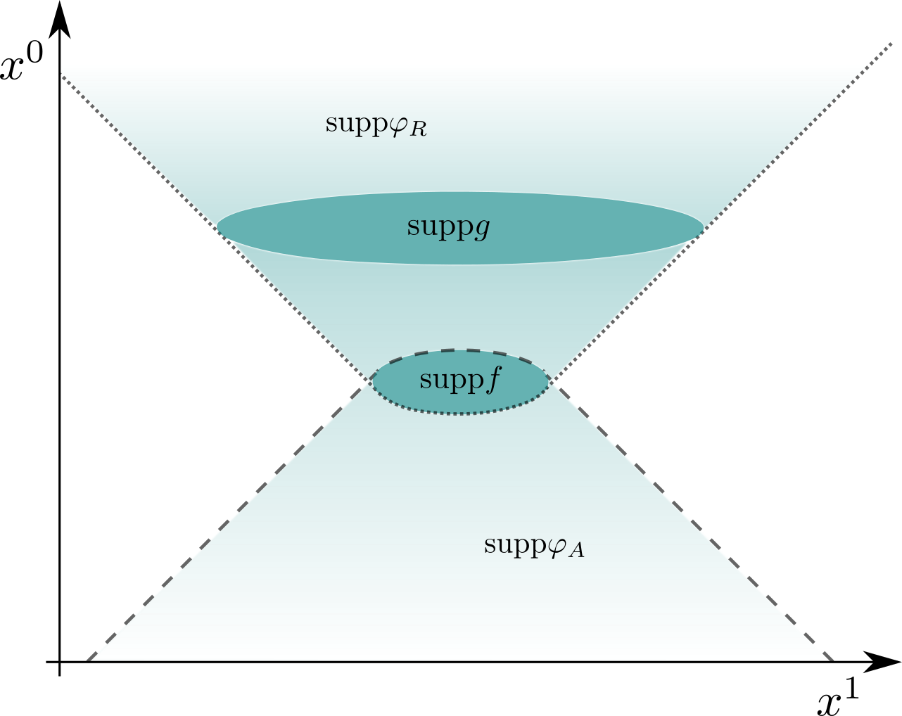
There is no unique that generates a spatially compact solution via . Two different test functions and that generate the same solution, i.e. , can even be supported in disjoint regions, as shown in Fig. 14. This lack of uniqueness appears in the quantum theory too, e.g. for any two test functions satisfying the classical equation . In Section II.2 this was stated in a different, but equivalent way, as for some test function . As stated in Section II.2, this is equivalent to imposing the homogeneous equations of motion on the operator-valued distribution in (1).
Given that the smeared field operators can be the same for different test functions, the region within which a smeared field is localisable is clearly not unique. The two regions in Fig. 14 are examples of possible localisation regions. This non-uniqueness is not completely arbitrary; starting from the smearing function for example, we cannot move the localisation region to a region spacelike to .

In practice we can ‘move’ the smeared field in the following way. Consider the test function supported in some compact subset , and the classical solution that it generates. Now consider some compact such that (Fig. 15), in which we want to localise . This amounts to the classical problem of finding some supported in that generates as . To do this we first choose any smooth partition of , i.e. , where the supports of and only intersect in , and vanishes to the past/future of . This is shown in Fig 15. Given the supports of it is clear that, to the future/past of , we have . Since satisfies the homogeneous equation in (102), then also satisfies (102) to the future/past of . Furthermore, trivially satisfies (102) to the past/future of as it vanishes there. Inside , however, may not satisfy (102). Let be the function capturing this inability of to satisfy (102) inside , i.e. . Note that is the same for both and , as the difference satisfies the homogeneous equation everywhere, including inside . By our previous arguments we also know that is compactly supported in . Furthermore, it is by definition a source for the past/future compact solution of the inhomogeneous equation, and hence we can write . Therefore, we have
| (106) |
That is, , and so is equivalent to in that they generate the same solution to the homogeneous equation. We therefore have the operator equality , and hence this smeared field operator is localisable in as desired. The above argument has glossed over some technical details explained more thoroughly in Fewster and Verch 2020.
Let us now turn on a self-interaction in some compact subset . Specifically, we modify the classical homogeneous equation to
| (107) |
where is the interaction parameter, and is some smooth function, supported in , which controls the interaction. Here we have picked a interaction (a interaction in the associated action) as an example. The explicit form of the interaction is not so important for our discussion, however, and so one can substitute in some other interaction in what follows.
From this compact we get the associated in- and out-regions . This is illustrated in Fig. 16. In the interaction is turned off, and hence the theory matches the free case. is also globally hyperbolic in its own right, and hence the quantum theory restricted to goes through as in Section II.2. In particular, for any functions and both supported in either or , we have , where is the same as in the free theory. Similarly, for any sequence of measurements/kicks all contained in either or , our previous results go through unchanged.

There will be a change, however, if is supported in say, and is supported in , as shown in Fig. 16. Crucial to our discussion on measurements and kicks is the commutator . Currently, this commutator is undefined, as belongs to the algebra of operators in the in-region , and to algebra in the out-region . To define this commutator we first have to map to some operator in the algebra for the out-region. This can be done as follows.
Given the test function supported in we can generate which solves the free homogeneous equation throughout the entirety of . Furthermore, trivially solves the interacting equation (107) in as the interaction vanishes there. The only region where we do not yet know the interacting solution is the future of , . There we can perturbatively construct the interacting solution order by order in . For instance, for we get the equation , and hence . Note that for in .
We now have the perturbative solution throughout all of , and hence all of . Since the theory is free in we can perturbatively find some , supported in , that generates the solution as in . Order by order we have , where each can be found using the above prescription, i.e. we partition , where the supports of and only intersect in some compact subset of , and then set . A example of is shown in Fig. 16. Note that is not linearly dependent on . That is, if , then it is not the case that .
In the quantum theory we then have the map between the smeared field operators for the in- and out-regions respectively. We have used the double-ended arrow as we can also map smeared fields from the out- to the in-region following the above procedure. Note this map is non-linear in the test functions. The full scattering map is an algebra homomorphism between the algebra of operators for the in- and out-regions, and is defined by extending the map between smeared fields to all sums and products in the obvious way. For example, . The commutator , for supported in the out region, is then defined by first mapping , and then computing within . Essentially, .
One may worry that the non-linear dependence of on affects our previous results on causality. In fact, this non-linear dependence is not relevant to the question of causality when measuring/kicking a smeared field. Consider equation (IV.2.1) where we showed that smeared field operations do not increase the support of some Weyl generator. There was supported in some compact subset, say, and was supported in a region . Imagine now that the compact subset , where the interaction is turned on, is situated between and as in Fig. 16. Specifically, and . To take this interaction into account in (IV.2.1) we simply need to swap for , where is supported in and is related to via the above scattering map. This can be done perturbatively, i.e. order by order in , if convergence is not guaranteed. This changes the precise form of the RHS of (IV.2.1) as a function of , and hence the precise effect of the operation on any future measurements. Crucially, however, it does not change the fact that the support of the Weyl generator has not increased, and hence the operation is still causal, even in the presence of this self-interaction. We can similarly argue, using (III.1), that self-interactions do not make smeared field kicks acausal.
This argument can be readily applied to other self-interactions, and even to interactions with other fields via the scattering map in Fewster and Verch 2020. In each case the precise form of changes, but importantly the support is never increased. In this sense we can say that interactions do not make the situation for causality violations ‘worse’ than the free case.
VI Discussion
VI.1 Future directions
Before discussing the implications of our results, there are a number of future directions to note. While we touched on the case of ideal measurements, the fact that they seem acausal for the simplest operators, i.e. the smeared fields, warrants further study. Many of our results also seem transformable into the probe framework in Fewster and Verch 2020; Fewster 2019; Bostelmann et al. 2021. It would be useful to construct an explicit dictionary between update maps and specific probe models, and to determine whether this is possible in general. The latter would be analogous to Stinespring’s Dilation Theorem Stinespring 1955, but with the added restrictions of locality and causality on the unitary map. On this point we note that our discussion of update maps using only the main field of interest, i.e. with no additional probe fields, is still useful in that it allows us to say which operators of the main (and only) field can be causally measured (in the standard sense of quantum theory) without reference to another probe field, specifically because we can associate to any operator an update map . Finally, it would be illuminating to also translate our results from the canonical picture into the path integral framework for quantum theory.
VI.2 Relation to continuous measurement models
We briefly note the relevance of the above results to continuous measurement models Brun 2000; Jacobs and Steck 2006. In these models Gaussian measurements of a chosen operator are enacted repeatedly, in intervals of duration . The limit is then taken to make the sequence of measurements effectively continuous. These models are useful in many applications, including feedback control (e.g. Bushev et al. 2006), where the results of the measurements are used to continuously update the Hamiltonian. For a lattice system one of the simplest cases to study is continuous measurements of operators local to a single site, e.g. local number operators as in Cao et al. 2019. Since such operators are local, in the sense that they commute with operators on different sites, their associated Gaussian measurements do not increase support, and hence are causal, c.f. Gaussian measurements of smeared fields. One can also consider models involving Gaussian measurements of operators that couple neighbouring sites. In this case the Gaussian measurements increase support, and are therefore acausal. For a non-relativistic lattice system this means that the Gaussian measurements cannot be implemented faster than the light-travel time between the neighbouring sites. This furnishes a fundamental lower bound on the measurement duration . That is, ‘continuous’ measurement models such as these can only ever be approximately continuous on timescales much larger than this lower bound. In practice this lower bound may be negligible compared to the timescales present in the lattice model, and hence the assumption of a continuum of measurements is justified.
VI.3 Physical implications
Returning to QFT, from a philosophical perspective our claim that only the generators can be measured may have important implications for the ontology of the theory. The conventional picture in quantum mechanics is that one can associate to any physical observable a self-adjoint (and gauge invariant) operator. In measuring this observable we usually expect two things from quantum theory: i) a probability distribution over the possible measurement outcomes of the observable, and ii) a map to update the state of the system. The latter is crucial in accurately reflecting the effect of the current measurement on any future measurements.
For a smeared field operator we meet these two requirements: the pdf over possible measurement outcomes is given explicitly in (IV.1), and we can update the state via the associated Gaussian update map, , since it is causal.
In the case of more complicated self-adjoint operators requirement ii) is not obviously met, as it seems the associated Gaussian update maps cannot be implemented without violating causality. In this way these operators do not correspond to observables in the usual sense. Requirement i) is still be met however, as expectation values and higher moments of any self-adjoint operators can be recovered from Gaussian measurements of smeared fields a la Section IV.7.
While the update map for some self-adjoint operator may not be possible, we can nevertheless meet requirement ii) by instead composing the (causality respecting) update maps for the relevant smeared fields used in the construction of (potentially with some symmetrisation).
In this way we can in fact associate to any self-adjoint operator a causality respecting update map, thus meeting the conventional requirements, i) and ii), of an observable in quantum theory. In doing this, however, we must understand that our use of the update maps for the relevant smeared fields implies that, physically speaking, we are really measuring the smeared fields , and not . The ‘measurement’ of should be thought of as secondary to the measurement of the smeared fields , in the sense that any expectation values, or higher moments, of are actually constructed after the fact, a la Section IV.7, using the outcomes of the measurements of each .
Depending on one’s preferred interpretation of quantum mechanics, or one’s preferred outlook on QFT, this may amount to a different ontology — a different picture of what is physically there. Specifically, one way to interpret (and extrapolate from) the above results is that smeared fields (and the identity) are the only physical observables, and that other self-adjoint operators in the algebra simply correspond to different ways to combine the outcomes resulting from measurements of smeared fields. This unconventional viewpoint, where all self-adjoint operators except the smeared fields and the identity are ‘culled’ from the list of QFT observables, necessitates further justification.
To illustrate how one could take this viewpoint we focus on the example in Section IV.4. That is, we have two smeared fields and , localisable in spacelike regions. If we perform two Gaussian measurements, one for and one for , the respective measurement outcomes, and , are distributed according to the joint pdf in (87). Now consider the self-adjoint operator . We know from Section IV.4 that is acausal. From the above discussion we can instead take the update map to be the composition of and , in which case the pdf over the possible outcome values for this measurement of , denoted by , is the product pdf over the variable (determined by the joint pdf over the dependent random variables and ). In this precise sense one could argue that is not an ‘independent’ observable in its own right. It does not, for example, come with its own pdf of the the form (IV.1).
VI.4 Comparison with non-relativistic quantum mechanics
To highlight how this deviates from our usual intuition, let us examine the analogous situation in non-relativistic quantum mechanics (NRQM). Consider the operator , where and are two commuting operators local to separate parts of a bipartite system, e.g. and for some and local to different parts of the system. In this case there is no reason to rule out the map in favour of the composition . In the QFT setting this is precisely what we have done.
To further emphasise the distinction between the QFT and NRQM, recall that the limit of a Gaussian map is an ideal measurement (for compact self-adjoint operators). Therefore, for some sufficiently small , the analogous statement in NRQM is that we cannot make an ideal measurement of , but we can make two ideal measurements of and (in either order). This is demonstrably not the case; ideal measurements of product operators such as are routinely considered in QI.
We have to be careful, though, in making this connection, as we are applying infinite dimensional continuum QFT results to the finite dimensional Hilbert space of the bipartite system. To properly emulate our support increasing Gaussian measurement of in NRQM we should at least consider an operator whose ideal measurement is support increasing, or equivalently, is one that enables a (subluminal) signal. Accordingly, we consider the operator on two qubits and (where denotes the Pauli- matrix). Note that and here. In Borsten et al. 2021 it was shown that an ideal measurement of enables a signal.
Even with this choice of it is still the case that we can perform the associated ideal measurement, and we do not need to resort to a composition of ideal measurements of and . This non-relativistic example, therefore, still differs from the QFT case. In the latter, a Gaussian measurement of is physically impossible, and one can only do Gaussian measurements of and separately. Why, then, are these two situations different, and how can we reconcile this? Furthermore, such a reconciliation seems necessary if NRQM is to arise as an effective description of QFT.
To answer these questions we must focus on how an ideal measurement of is realised experimentally. As mentioned in Borsten et al. 2021, one can use the following 2 step LOCC (Local Operations and Classical Communication) protocol: 1) The experimenter first measures the -spin on qubit . 2) If it is down then they do nothing on qubit , and if it is up then they measure the -spin of qubit . One can verify that the associated sequence of update maps amounts to the update map for an ideal measurement of .
Notably, this realisation requires information about the measurement outcome on qubit to be sent to qubit before qubit is (potentially) measured. The spacetime regions in which the measurements of each qubit take place are therefore timelike related, and not spacelike. This is the crucial distinction to the QFT case. There the operators and are localisable in spacelike regions, and even if we ‘move’ the smeared fields around to and say, using the procedure in Section V, we can never make them totally timelike related, i.e. such that there are no pairs of points, and , that are spacelike. This is essentially why the two situations are different; why an ideal measurement of is possible in NRQM but a Gaussian measurement of in QFT is not.
Given that the two qubit measurements are totally timelike, the NRQM example is then more comparable to the Gaussian LOCC protocol in Section IV.8, which we found to be causal. This should provide some reassurance as to why our QFT results are not contradictory with standard NRQM experiments. From a QFT perspective, the update map for an ideal measurement of is physically realisable because it is simply an effective description of some underlying causal update map in the QFT setting.
This is not obvious from the form of the operator, , however. Given that and are local to separate parts of the tensor product we get the impression that they are analogous to spacelike observables in QFT. This led us to incorrectly compare with , where and are spacelike. ‘Hidden’ in the ideal measurement of is knowledge that the measurements of the two qubits happen in timelike regions. To make the situation more comparable to we can instead ask if the measurement of can be performed using spacelike qubit measurements. In other words, can we perform an ideal measurement of faster than the light-travel time between the qubits? This, like a Gaussian measurement of , is impossible. As shown in Borsten et al. 2021, if we were to make such a measurement of we would enable a superluminal signal, and hence it is impossible.
In this way, the conclusion that a Gaussian measurement of is impossible, and hence why (and many other operators) fail requirement ii) for a typical observable in quantum theory, is more reasonable. Ruling out as unobservable is analogous to ruling out as unobservable on time-scales shorter than its light-travel time – the latter being perfectly reasonable to those in QI.
VII Conclusion
Above we precisely formulated Sorkin’s additional causality condition that any state update in QFT should obey to respect causality. Through the use of unitary kicks with smeared fields we showed that causal state updates in real scalar QFT are precisely those that are past-support non-increasing (PSNI). Moreover, we argued that PSNI state updates are causal more generally, specifically for the physical subalgebras of complex scalar and fermionic QFT. We then went on to consider a variety of update maps in real scalar QFT with a focus on Gaussian measurements. Our calculations suggest that only Gaussian measurements/unitary kicks with the generators (the smeared fields and the identity) are causal, while measurements/kicks with other more complicated operators are acausal. Additionally, ideal measurements of smeared fields appear to be acausal, though a more thorough analysis needs to be done. Using Gaussian measurements of smeared fields alone we then sketched how one could recover expectation values of products of smeared fields, and following this we discussed the addition of a compactly supported interaction.
In the last section we discussed some future directions and relations to continuous measurement models. We then went on to discuss the physical implications of our findings, arguing that the generators of the algebra seem to be the only physical observables, at least in the usual sense of quantum physics. Despite our above reasoning, a shift in ontology as radical as culling all self-adjoint operators, bar smeared fields and the identity, from the list of QFT observables certainly requires further scrutiny before it should be taken seriously. In particular, we have only focussed on a few particular classes of update maps, and even within the set of these maps there are more LOCC protocols that can be investigated.
Lastly, while this potential shift in ontology would not obviously be of any practical importance, it may be relevant in the construction of more fundamental theories. Specifically, a clearer understanding of what is physical in curved spacetime QFT will, most likely, better inform our decisions as to which physical principles to retain in quantum gravity.
Acknowledgements: The author would like to acknowledge L. Borsten, G. Kells, L. Coopmans, A. Conlon, M. Ruep, C. Fewster, and N. Curran for helpful discussions, as well as the referee for many helpful suggestions. IJ is supported by a Schrödinger Scholarship.
References
- (1) Here we work in the Heisenberg picture where operators carry the dynamics, and hence it makes sense to talk about operators at points, or more accurately in regions, of spacetime.
- Hellwig and Kraus (1970) K. E. Hellwig and K. Kraus, Formal description of measurements in local quantum field theory, Phys. Rev. D 1, 566 (1970).
- Sorkin (1993) R. D. Sorkin, Impossible measurements on quantum fields, in Directions in General Relativity: An International Symposium in Honor of the 60th Birthdays of Dieter Brill and Charles Misner (1993) arXiv:gr-qc/9302018 .
- Benincasa et al. (2014) D. M. T. Benincasa, L. Borsten, M. Buck, and F. Dowker, Quantum information processing and relativistic quantum fields, Classical and Quantum Gravity 31, 075007 (2014).
- Borsten et al. (2021) L. Borsten, I. Jubb, and G. Kells, Impossible measurements revisited (2021), arXiv:1912.06141 [quant-ph] .
- Beckman et al. (2002) D. Beckman, D. Gottesman, A. Kitaev, and J. Preskill, Measurability of wilson loop operators, Phys. Rev. D 65, 065022 (2002).
- (7) Note we are not saying that the analogous state updates in NRQM are impossible, just that this is the case in relativistic QFT.
- Tjoa and Martín-Martínez (2019) E. Tjoa and E. Martín-Martínez, Zero mode suppression of superluminal signals in light-matter interactions, Physical Review D 99, 10.1103/physrevd.99.065005 (2019).
- Martín-Martínez et al. (2021) E. Martín-Martínez, T. R. Perche, and B. d. S. Torres, Broken covariance of particle detector models in relativistic quantum information, Physical Review D 103, 10.1103/physrevd.103.025007 (2021).
- de Ramón et al. (2021) J. de Ramón, M. Papageorgiou, and E. Martín-Martínez, Relativistic causality in particle detector models: Faster-than-light signaling and impossible measurements, Physical Review D 103, 10.1103/physrevd.103.085002 (2021).
- Perche and Martín-Martínez (2021) T. R. Perche and E. Martín-Martínez, Anti-particle detector models in qft (2021), arXiv:2106.03874 [quant-ph] .
- Polo-Gómez et al. (2021) J. Polo-Gómez, L. J. Garay, and E. Martín-Martínez, A detector-based measurement theory for quantum field theory (2021), arXiv:2108.02793 [quant-ph] .
- Beckman et al. (2001) D. Beckman, D. Gottesman, M. A. Nielsen, and J. Preskill, Causal and localizable quantum operations, Phys. Rev. A 64, 052309 (2001).
- Popescu and Vaidman (1994) S. Popescu and L. Vaidman, Causality constraints on nonlocal quantum measurements, Physical Review A 49, 4331–4338 (1994).
- Martín-Martínez (2015) E. Martín-Martínez, Causality issues of particle detector models in qft and quantum optics, Physical Review D 92, 10.1103/physrevd.92.104019 (2015).
- Bostelmann et al. (2021) H. Bostelmann, C. J. Fewster, and M. H. Ruep, Impossible measurements require impossible apparatus, Physical Review D 103, 10.1103/physrevd.103.025017 (2021).
- (17) This follows as is a rank 1 operator, and so cannot be localisable in any spacetime region, as all localisable projectors must be of infinite rank — a common feature of type III von Neumann algebras (see Fewster and Rejzner 2019 for example).
- Fewster and Verch (2020) C. J. Fewster and R. Verch, Quantum fields and local measurements, Communications in Mathematical Physics 378, 851 (2020).
- Fewster (2019) C. J. Fewster, A generally covariant measurement scheme for quantum field theory in curved spacetimes (2019), arXiv:1904.06944 [gr-qc] .
- Ruep (2021) M. H. Ruep, Weakly coupled local particle detectors cannot harvest entanglement (2021), arXiv:2103.13400 [quant-ph] .
- Brun (2000) T. A. Brun, Continuous measurements, quantum trajectories, and decoherent histories, Physical Review A 61, 10.1103/physreva.61.042107 (2000).
- Jacobs and Steck (2006) K. Jacobs and D. A. Steck, A straightforward introduction to continuous quantum measurement, Contemporary Physics 47, 279–303 (2006).
- Fewster and Rejzner (2019) C. J. Fewster and K. Rejzner, Algebraic quantum field theory – an introduction (2019), arXiv:1904.04051 [hep-th] .
- Wald (1984) R. M. Wald, General relativity (Chicago Univ. Press, Chicago, IL, 1984).
- Haag (1996) R. Haag, Local quantum physics: Fields, particles, algebras (Springer-Verlag, Berlin, 1996).
- Araki (1964) H. Araki, Von neumann algebras of local observables for free scalar field, Journal of Mathematical Physics 5, 1 (1964), https://doi.org/10.1063/1.1704063 .
- (27) In what follows we will implicitly restrict to states for which such expectation values are well defined, specifically quasifree states (described in the AQFT framework in Fewster and Rejzner 2019) and any states that can be constructed from these via the action of elements in .
- (28) Note that these two approaches are only equivalent given a suitable representation of the algebra. We meet this requirement through our use of the usual bosonic Fock space and our implicit assumption of an appropriate ground state on which the Fock space is built.
- Baker (1905) H. F. Baker, Alternants and continuous groups, Proceedings of the London Mathematical Society s2-3, 24 (1905).
- Campbell (1897) J. E. Campbell, On a law of combination of operators (second paper)*, Proceedings of the London Mathematical Society s1-29, 14 (1897).
- Hausdorff (1906) F. Hausdorff, Die symbolische Exponentialformel in der Gruppentheorie, Ber. Verh. Kgl. Sächs. Ges. Wiss. Leipzig., Math.-phys. Kl. 58, 19 (1906).
- Casas and Murua (2009) F. Casas and A. Murua, An efficient algorithm for computing the baker–campbell–hausdorff series and some of its applications, Journal of Mathematical Physics 50, 033513 (2009).
- Reed and Simon (1981) M. Reed and B. Simon, I: Functional Analysis, Methods of Modern Mathematical Physics (Elsevier Science, 1981).
- (34) The spectrum of a smeared field , like the position operator in NRQM, is the whole of .
- Stinespring (1955) W. F. Stinespring, Positive functions on c*-algebras, Proceedings of the American Mathematical Society 6, 211 (1955).
- Bushev et al. (2006) P. Bushev, D. Rotter, A. Wilson, F. m. c. Dubin, C. Becher, J. Eschner, R. Blatt, V. Steixner, P. Rabl, and P. Zoller, Feedback cooling of a single trapped ion, Phys. Rev. Lett. 96, 043003 (2006).
- Cao et al. (2019) X. Cao, A. Tilloy, and A. De Luca, Entanglement in a fermion chain under continuous monitoring, SciPost Physics 7, 10.21468/scipostphys.7.2.024 (2019).