Pattern recognition in Deep Boltzmann machines

E. Agliari Affiliation: Dipartimento di Matematica Guido Castelnuovo, Sapienza Università di Roma, Rome, Italy Affiliation: Istituto Nazionale d’Alta Matematica Francesco Severi, Rome, Italy L. Albanese Affiliation: Istituto Nazionale d’Alta Matematica Francesco Severi, Rome, Italy Affiliation: Dipartimento di Matematica e Fisica Ennio De Giorgi, Università del Salento, Lecce, Italy F. Alemanno Affiliation: Istituto Nazionale d’Alta Matematica Francesco Severi, Rome, Italy Affiliation: Dipartimento di Matematica e Fisica Ennio De Giorgi, Università del Salento, Lecce, Italy A. Fachechi Affiliation: Istituto Nazionale d’Alta Matematica Francesco Severi, Rome, Italy Affiliation: Dipartimento di Matematica e Fisica Ennio De Giorgi, Università del Salento, Lecce, Italy Affiliation: Istituto Nazionale di Fisica Nucleare, Campus Ecotekne, Lecce,Italy

Abstract

We consider a multi-layer Sherrington-Kirkpatrick spin-glass as a model for deep restricted Boltzmann machines and we solve for its quenched free energy, in the thermodynamic limit and allowing for a first step of replica symmetry breaking. This result is accomplished rigorously exploiting interpolating techniques and recovering the expression already known for the replica-symmetry case. Further, we drop the restriction constraint by introducing intra-layer connections among spins and we show that the resulting system can be mapped into a modular Hopfield network, which is also addressed rigorously via interpolating techniques up to the first step of replica symmetry breaking.

1 Introduction

Restricted Boltzmann machines (RBMs) constitute a popular model in machine learning (see e.g., [1, 2, 3]) due to a relatively easy architecture (a RBM consists of one visible layer and one hidden layer with interlayer interactions only) and to its analogies with bipartite spin-glass models which allow for theoretical investigations and a mathematical control [4, 5, 6, 7, 8]. A more challenging version of the RBM is given by the Deep Boltzmann machine (DBM), which comprises a set of hidden layers, see Fig. 1 In the statistical-mechanics of disordered-system jargon, this can be considered as a multi-layer spin-glass where the set of spins is arranged into a geometry made of consecutive layers and only interactions among spins belonging to adjacent layers are allowed. Also motivated by the impressive successes obtained in artificial intelligence via deep learning methods (which, beyond DBMs include a number of other different neural networks), this kind of structures have recently attracted a wide interest (see e.g., [9, 10, 11, 12, 13, 14]).
Here, we consider a multi-layer spin-glass, specifically, a multi-layer Sherrington-Kirkpatrick (MSK) model and we solve for its free-energy via interpolating techniques: the free energy is expressed in terms of interpolating parameters $(t,\vec{x})$ , meant as time and space variables, and it is shown to fulfil a transport-like equations; an explicit expression for the original free energy can then be obtained by solving a partial differential equations and suitably setting the parameters $(t,\vec{x})$ . Exploiting this technique and assuming replica-symmetry (RS), we recover the result previously found in [9] for multi-layer spin-glasses and, further, our approach allows us to obtain a refined picture which includes replica-symmetry breaking; only the first step (1RSB) is addressed in details, the generalisation works analogously [15].
Next, we move to a more complex architecture, where we introduce an additional class of spins, one for each couple of adjacent layers and bridging the related spins, see Fig. 2 (left panel). The interest in this kind of structure lays in the fact that, as we prove, it is formally equivalent to a modular Hopfield model, also referred to as deep Hopfield network (DHN) see Fig. 2 (right panel). Indeed, in the past years, following experimental evidences about the existence of sub-units in brain networks (see e.g., [16, 17, 18, 19]) associative neural networks embedded in modular topologies have attracted much attention [20, 21, 22, 23, 24]. Here, exploiting the above-mentioned interpolating techniques, we solve for the free energy of a Hopfield model made of several sub-units, each made of fully-connected neurons. We first address the problem under the replica-symmetry assumption and then we extend the treatment to the first-step of replica symmetry breaking.

2 The transport equation for the DBM

In this section we focus on the MSK model as a formal representation of the DBM: first, in sec. 2.1, we formally introduce the model and the related observables, next, in sec. 2.2 we prove that its interpolating quenched pressure fulfils a transport-like equation and finally, in secs. 2.3-2.4 we obtain a solution of such an equation – under, respectively, the RS and the 1RSB assumption – and, by suitably setting the interpolating parameters, we get an explicit expression for the MSK quenched pressure in the thermodynamic limit.

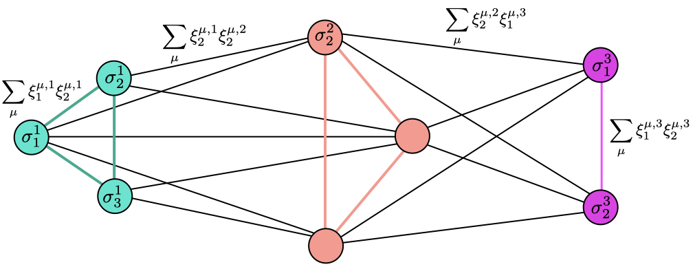
Figure 1: Schematic representation of a restricted DBM, made of

K

layers of size

N_{1}=5

N_{2}=3

, …,

N_{K}=4

. Spins belonging to adjacent layers are completely connected pairwisely. Notation is specified only for a few spins and links in order to ensure readability.

Refer to caption — Figure 2: Left: Schematic representation of a DBM, made of $K=3$ layers (the depth is limited for readability purposes), made of $N_{1}=N_{2}=3$ and $N_{3}=2$ spins; spins belonging to adjacent layers, say layers $p$ and $p+1$ are connected to the hidden neuron $z_{p}$ , thus, the overall number of hidden neurons is $K-1$ . Right: Schematic representation of a DHM, corresponding to the DBM on the left; this is made of $K=3$ layers of size $N_{1}=N_{2}=3$ and $N_{3}=2$ . Each layer includes spins that are fully connected each other, further, spins belonging to adjacent layers are completely connected each other. In both panels notation for spins and weights is reported only in few cases to ensure readability.

2.1 Definitions

Definition 1.

Let us consider a multilayer Sherrington-Kirkpatrick (MSK) model of size $N$ and endowed with $K$ layers, each made of $N_{p}$ binary spins, with $N_{p}=\lambda_{p}N$ , for $p=1,...,K$ , then $\sum_{p=1}^{K}\lambda_{p}=1$ ; interactions are pairwise and only involve spins belonging to adjacent layers, in such a way that the Hamiltonian of the model reads as

H_{N,K}(\sigma;J):=-\sqrt{\frac{2}{N}}\sum_{p=1}^{K-1}\sum_{i,j=1}^{N_{p},N_{p+1}}J_{ij}^{p}\sigma^{p}_{i}\sigma^{p+1}_{j},

(2.1)

where $\bm{\sigma}^{p}=(\sigma_{1}^{p},...,\sigma_{N_{p}}^{p})\in\{-1,+1\}^{N_{p}}$ for $p=1,...,K$ and the matrix $\bm{J}^{p}$ has size $N_{p}\times N_{p+1}$ with entries that are standard Gaussian, that is $J^{p}_{ij}\sim\mathcal{N}(0,1)$ for $i=1,...,N_{p}$ , $j=1,...,N_{p+1}$ , $p=1,...,K-1$ .

Definition 2.

The partition function of the MSK model defined in (1) is given by

Z_{N,K}(\beta,J):=\sum_{\bm{\sigma}}e^{-\beta H_{N,K}(\sigma;J)}=\sum_{\bm{\sigma}}e^{\beta\sqrt{\frac{2}{N}}\sum_{p=1}^{K-1}\sum_{i,j=1}^{N_{p},N_{p+1}}J_{ij}^{p}\sigma^{p}_{i}\sigma^{p+1}_{j}},

(2.2)

where $\beta$ is the inverse temperature and the sum runs over all spin configurations, that is $\bm{\sigma}=(\bm{\sigma}^{1},\bm{\sigma}^{2},...,\bm{\sigma}^{K})\in\{-1,+1\}^{N}$ .

Definition 3.

The quenched, intensive pressure of the MSK model defined in (1) with partition function given by (2.2) is defined as

A_{N,K}(\beta):=\frac{1}{N}\mathbb{E}_{J}\log Z_{N,K}(\beta,J),

(2.3)

where $\mathbb{E}_{J}$ stands for the quenched averaging operator acting as $\mathbb{E}_{J}f(\mathbf{J}):=\int\prod_{p=1}^{K+1}\left(\frac{dJ^{p}}{\sqrt{2\pi}}e^{-(J^{p})^{2}/2}\right)\penalty\ f(\mathbf{J})$ $\mathbf{J}=(\bm{J}^{1},\bm{J}^{2},\dots,\bm{J}^{K-1})$ . We recall that the pressure equals the free energy, a constant $-\beta$ apart.

Definition 4.

For the generic observable $O(\bm{\sigma})$ , the Boltzmann-Gibbs average stemming from (2.2) is defined as

\langle O\rangle:=\frac{1}{Z_{N,K}(\beta,J)}\sum_{\sigma}O(\bm{\sigma})e^{-\beta H_{N,K}(\sigma;J)}.

(2.4)

In relation to the Boltzmann-Gibbs average we also introduce the $\Delta$ operator for the observable $O(\bm{\sigma})$ as

\Delta[O(\bm{\sigma})]:=O(\bm{\sigma})-\lim_{N\to\infty}\mathbb{E}_{J}\langle O\rangle.

(2.5)

In the following, we will often move to the thermodynamic limit $N\to\infty$ , still retaining $K$ finite. In order to highlight that a quantity is evaluated in the thermodynamic limit, we will drop the dependence on $N$ and, in particular,

A_{K}(\beta):=\lim_{N\to\infty}A_{N,K}(\beta).

(2.6)

2.2 Mechanical Analogy

In this subsection we introduce an interpolating pressure $\mathcal{A}_{N,K}(t,\vec{x})$ depending on the interpolating parameters $t\in\mathbb{R}^{+}$ and $\vec{x}\in\mathbb{R}^{K}$ , which can be interpreted as, respectively, time and space variables, and such that $A_{N,K}(\beta)=\mathcal{A}_{N,K}(t=\beta^{2},\vec{x}=0)$ ; next, we will show that $\mathcal{A}_{N,K}(t,\vec{x})$ fulfills a transport equation, whose solution, evaluated in $t=\beta^{2}$ and $\vec{x}=0$ , therefore provides the pressure for the original MSK.

Definition 5.

The interpolating pressure $\mathcal{A}_{N,K}(t,\vec{x})$ for the MSK model (1), also referred to as Guerra Action, is defined as

\begin{split}\mathcal{A}_{N,K}(t,\vec{x}):=\frac{1}{N}\mathbb{E}_{J}\log\sum_{\bm{\sigma}}\exp\Big(\sqrt{t}\sqrt{\frac{2}{N}}\sum_{p=1}^{K-1}\sum_{i,j=1}^{N_{p},N_{p+1}}J_{ij}^{p}\sigma^{p}_{i}\sigma^{p+1}_{j}+\sum_{p=1}^{K}\sqrt{x_{p}}\sum_{i=1}^{N_{p}}J^{p}_{i}\sigma^{p}_{i}\Big),\end{split}

(2.7)

where $t\in\mathbb{R}^{+}$ , $\vec{x}=(x_{1},...,x_{K})\in\mathbb{R}^{K}$ , and $J^{p}=(J_{1}^{p},...,J_{N_{p}}^{p})$ , with $J_{i}^{p}\sim\mathcal{N}(0,1)$ for $i=1,...,N_{p}$ and $p=1,...,K$ . Here, $\mathbb{E}_{J}$ stands for the averaging operator acting on both the original $J_{ij}^{p}$ couplings and the $J_{i}^{p}$ auxiliary random variables.

Remark 1.

Notice that, for $t=\beta^{2}$ and $\vec{x}=0$ , we exactly recover the pressure (2.3) for the original model.

Definition 6.

Given two replicas of the system, labelled as $a$ and $b$ , and characterized by the same realization of quenched disorder $\{\bm{J}^{p}\}_{p=1,...,K-1}$ , we define the two-replica overlap related to the $p$ -th layer as

q^{p}_{ab}(\bm{\sigma}^{p,(a)},\bm{\sigma}^{p,(b)})=\frac{1}{N_{p}}\sum_{i=1}^{N_{p}}\sigma_{i}^{p,(a)}\sigma_{i}^{p,(b)},\quad\quad p=1,...,K,

(2.8)

and these quantities play as order parameters for the MSK model.

Lemma 1.

The partial derivatives of the Guerra Action w.r.t. $t$ and each $x_{p}$ yield to the following expectation values:

	$\displaystyle\frac{\partial\mathcal{A}_{N,K}}{\partial t}$	$\displaystyle=$	$\displaystyle\sum_{p=1}^{K-1}\lambda_{p}\lambda_{p+1}(1-\mathbb{E}_{J}\langle q^{p}_{12}q^{p+1}_{12}\rangle),$		(2.9)
	$\displaystyle\frac{\partial\mathcal{A}_{N,K}}{\partial x_{p}}$	$\displaystyle=$	$\displaystyle\frac{\lambda_{p}}{2}\big[1-\mathbb{E}_{J}\langle q^{p}_{12}\rangle\big],$		(2.10)

where now, with a little abuse of notation, the thermodynamic average $\langle\cdot\rangle$ refers to the interpolating system.

Proof.

The explicit computation of the derivative $\partial_{t}A_{N,K}$ leads to

\partial_{t}\mathcal{A}_{N,K}=\frac{1}{N}\frac{1}{2\sqrt{t}}\sqrt{\frac{2}{N}}\sum_{p=1}^{K-1}\sum_{i,j=1}^{N_{p},N_{p+1}}\mathbb{E}_{J}J_{ij}^{p}\langle\sigma^{p}_{i}\sigma^{p+1}_{j}\rangle,

(2.11)

thus, applying Wick’s Theorem for Gaussian averages, we obtain

\begin{split}\partial_{t}\mathcal{A}_{N,K}&=\frac{1}{N}\frac{1}{2\sqrt{t}}\sqrt{\frac{2}{N}}\sum_{p=1}^{K-1}\sum_{i,j=1}^{N_{p},N_{p+1}}\mathbb{E}_{J}\partial_{J_{ij}^{p}}\langle\sigma^{p}_{i}\sigma^{p+1}_{j}\rangle=\frac{1}{N^{2}}\sum_{p=1}^{K-1}\sum_{i,j=1}^{N_{p},N_{p+1}}\mathbb{E}_{J}\big(1-\langle\sigma^{p}_{i}\sigma^{p+1}_{j}\rangle^{2}\big).\end{split}

(2.12)

Upon using (2.8), we directly obtain (2.9). The computation of the spatial derivative (2.10) follows the same lines, thus we omit the proof. ∎

Remark 2.

We introduce the variables $\lambda_{0}=\lambda_{K+1}=0$ in order to present the following equations in a more symmetrical fashion.

Proposition 1.

At finite $N$ , the Guerra Action (2.7) obeys to the following PDE:

\frac{\partial\mathcal{A}_{N,K}}{\partial t}-2\sum_{p=1}^{K}(\lambda_{p-1}q^{p-1}+\lambda_{p+1}q^{p+1})\frac{\partial\mathcal{A}_{N,K}}{\partial x_{p}}=S_{N}(t,\vec{x})+V_{N}(t,\vec{x}),

(2.13)

where we defined

q^{p}:=\lim_{N\to\infty}\mathbb{E}_{J}\langle q^{p}_{12}\rangle,\quad\quad p=1,...,K,

(2.14)

and

	$\displaystyle S_{N}(t,\vec{x})$	$\displaystyle:=$	$\displaystyle\sum_{p=1}^{K}\lambda_{p}\lambda_{p+1}(1-q^{p}-q^{p+1}+q^{p}q^{p+1}),$		(2.15)
	$\displaystyle V_{N}(t,\vec{x})$	$\displaystyle:=$	$\displaystyle-\sum_{p=1}^{K}{\lambda_{p}\lambda_{p+1}}{}\mathbb{E}_{J}\langle\Delta[q^{p}_{12}]\,\Delta[q^{p+1}_{12}]\rangle,$		(2.16)

are respectively the “source” and “potential” terms.

Proof.

The proof works by direct use of equations (2.9) and (2.10). First of all, we express the correlation function of the two overlaps in terms of the averages of the fluctuations, i.e. adopting the decomposition

\langle q^{p}_{12}q^{p+1}_{12}\rangle=-q^{p}q^{p+1}+q^{p}\langle q^{p+1}_{12}\rangle+q^{p+1}\langle q^{p}_{12}\rangle+\langle\Delta[q^{p}_{12}]\Delta[q^{p+1}_{12}]\rangle.

(2.17)

Inserting this relation in (2.9), we reach

\frac{\partial\mathcal{A}_{N,K}}{\partial t}=\sum_{p=1}^{K-1}\lambda_{p}\lambda_{p+1}-\mathbb{E}_{J}\sum_{p=1}^{K-1}\lambda_{p}\lambda_{p+1}\big(-q^{p}q^{p+1}+q^{p}\langle q^{p+1}_{12}\rangle+q^{p+1}\langle q^{p}_{12}\rangle+\langle\Delta[q^{p}_{12}]\Delta[q^{p+1}_{12}]\rangle\big).

The single-overlap expectation values (i.e. $\langle q_{12}^{p}\rangle$ and $\langle q_{12}^{p+1}\rangle$ ) can be expressed in terms of the spatial derivatives of the Guerra Action by reverting (2.10). The remaining contributions, involving expectation values of the fluctuations and a polynomial function of the parameters $q^{p}$ , are respectively condensed in source and the potential contribution. Thus, with simple algebra we reach the thesis (2.13). ∎

Remark 3.

The solution of the PDE (2.13) can be addressed by means of the method of characteristics. This suggests to consider the spatial coordinated $\vec{x}$ as a function of $t$ such that $\dot{x}_{p}:=dx_{p}/dt=-2(\lambda_{p-1}q^{p-1}+\lambda_{p+1}q^{p+1})$ , for $p=1,...,K$ . With this choice, the PDE in Eq. (2.13) can be recast into an evolutive ODE as

\frac{d\mathcal{A}_{N,K}}{dt}=S_{N}(t,\vec{x})+V_{N}(t,\vec{x}).

(2.18)

2.3 Replica Symmetric Solution

In this section, we find an explicit solution for $A_{K}(\beta)$ under the replica symmetry (RS) assumption.

Definition 7.

Under the replica-symmetry assumption, the distribution of the two-replica overlap $q^{p}_{12}$ converges in the thermodynamic limit to a Dirac delta centered at the equilibrium value $\bar{q}^{p}$ , that is

\lim_{N\rightarrow+\infty}P_{N}(q_{12}^{p})=\delta(q_{12}^{p}-\bar{q}^{p}),\penalty\ \penalty\ \textrm{for}\penalty\ p=1,...,K.

(2.19)

Proposition 2.

In the thermodynamic limit and under the RS assumption, the Guerra Action is given by

\begin{split}\mathcal{A}^{{\rm\scriptscriptstyle RS}}_{K}(t,\vec{x})=\log 2&+\sum_{p=1}^{K}\lambda_{p}\mathbb{E}_{J}\log\cosh\left[J\sqrt{x_{p}+2t(\lambda_{p-1}\bar{q}^{p-1}+\lambda_{p+1}\bar{q}^{p+1})}\right]\\ &+t\sum_{p=1}^{K}\lambda_{p}\lambda_{p+1}(1-\bar{q}^{p}-\bar{q}^{p+1}+\bar{q}^{p}\bar{q}^{p+1}).\end{split}

(2.20)

Proof.

Under the RS assumption, the fluctuations of the order parameters w.r.t. to their equilibrium value vanish in the thermodynamic limit, meaning that ${\Delta[q_{12}^{p}]}\overset{N\to\infty}{\longrightarrow}0$ , for any $p$ . Thus, recalling the definition (2.16), we have $V_{N}\overset{N\to\infty}{\longrightarrow}0$ . The PDE (2.13) therefore becomes the transport equation

\frac{\partial\mathcal{A}^{{\rm\scriptscriptstyle RS}}_{K}}{\partial t}-2\sum_{p=1}^{K}(\lambda_{p-1}\bar{q}^{p-1}+\lambda_{p+1}\bar{q}^{p+1})\frac{\partial\mathcal{A}^{{\rm\scriptscriptstyle RS}}}{\partial x_{p}}=S^{{\rm\scriptscriptstyle RS}}(t,\vec{x}).

(2.21)

where now $S^{{\rm\scriptscriptstyle RS}}(t,\vec{x})=\sum_{p=1}^{K}\lambda_{p}\lambda_{p+1}(1-\bar{q}^{p}-\bar{q}^{p+1}+\bar{q}^{p}\bar{q}^{p+1})$ because of the RS assumption (2.19). This equation can be readily solved by means of the method of characteristics, from which we find that

\mathcal{A}_{K}^{{\rm\scriptscriptstyle RS}}\big(t,\vec{x}\big)=\mathcal{A}_{K}^{{\rm\scriptscriptstyle RS}}\big(0,\vec{x}_{0}\big)+tS^{{\rm\scriptscriptstyle RS}}(t,\vec{x}),

(2.22)

where $\vec{x}_{0}:=\vec{x}(t=0)$ with generic $p$ -th component

\begin{split}x_{0,p}=x_{p}+2t(\lambda_{p-1}\bar{q}^{p-1}+\lambda_{p+1}\bar{q}^{p+1}).\end{split}

(2.23)

The initial condition $\mathcal{A}_{K}^{\rm\scriptscriptstyle RS}\big(0,\vec{x}_{0}\big)$ can be explicitly obtained by using the definition (2.7), since at $t=0$ the two-body contribution disappears. In this case, the computation of the Guerra Action is straightforward (since it reduces to a 1-body model), and leads to

\begin{split}\mathcal{A}_{N,K}(0,\vec{x}_{0})=\frac{1}{N}\mathbb{E}_{J}\log\sum_{\bm{\sigma}}\exp\Big(\sum_{p=1}^{K}\sqrt{x_{0,p}}\sum_{i=1}^{N_{p}}J^{p}_{i}\sigma^{p}_{i}\Big)=\log 2+\sum_{p=1}^{K}\lambda_{p}\mathbb{E}_{J}\log\cosh(J\sqrt{x_{0,p}}).\end{split}

(2.24)

We stress that, once the sum over all possible configurations is taken, we end up with the product of averages of identically distributed functions of the auxiliary variables $J_{i}^{p}$ , so we can drop both the spin and layer indices and use a single random variable $J$ on which the average $\mathbb{E}_{J}$ is performed. Putting the two pieces together and using (2.23), we obtain the thesis (2.20). ∎

Theorem 1.

The replica-symmetric intensive quenched pressure in the thermodynamic limit for the MSK model is recovered [9]:

\begin{split}A_{K}^{{\rm\scriptscriptstyle RS}}\big(\beta)=\log 2&+\sum_{p=1}^{K}\lambda_{p}\mathbb{E}_{J}\log\cosh(J\beta\sqrt{2}\sqrt{\lambda_{p-1}\bar{q}^{p-1}+\lambda_{p+1}\bar{q}^{p+1}})+\beta^{2}\sum_{p=1}^{K}\lambda_{p}\lambda_{p+1}(1-\bar{q}^{p})(1-\bar{q}^{p+1}).\end{split}

(2.25)

Proof.

The result follows by simply setting $t=\beta^{2}$ and $\vec{x}=0$ in (2.20). ∎

Corollary 1.

The replica-symmetric expectation of the order parameters $\bar{q}_{12}^{p}$ obeys the following self-consistent equation:

\bar{q}^{p}=\mathbb{E}_{J}\tanh^{2}\big[\beta J\sqrt{2(\lambda_{p-1}\bar{q}^{p-1}+\lambda_{p+1}\bar{q}^{p+1})}\big],\quad\quad p=1,...,K.

(2.26)

Proof.

To prove this result, as usual in disorder statistical mechanics, we extremize $A_{K}^{{\rm\scriptscriptstyle RS}}(\beta)$ w.r.t all order parameters: $\partial A_{K}^{{\rm\scriptscriptstyle RS}}(\beta)/\partial\bar{q}^{p}=0$ for all $p=1,\dots,K$ . With straightforward computations, we find that extremality conditions implies

\begin{split}&\lambda_{p}\lambda_{p+1}(\bar{q}^{p+1}-\mathbb{E}_{J}\tanh^{2}[\beta J\sqrt{2(\lambda_{p}q^{p}+\lambda_{p+2}q^{p+2})}])\\ +&\lambda_{p}\lambda_{p-1}(\bar{q}^{p-1}-\mathbb{E}_{J}\tanh^{2}[\beta J\sqrt{2(\lambda_{p}q^{p}+\lambda_{p-2}q^{p-2})}])=0.\end{split}

(2.27)

Since these constraints hold for general $\lambda_{p}$ , we must set to zero the quantities in round brackets, which directly leads to the thesis (2.26). ∎

2.4 1RSB solution

In this section we find an explicit solution for $A_{K}(\beta)$ under the 1RSB assumption which can be stated as

Definition 8.

In the first step of replica-symmetry breaking, the distribution of the two-replica overlap $q_{12}^{p}$ in the thermodynamic limit displays two delta-peaks at the equilibrium values, referred to as $\bar{q}_{1}^{p},\ \bar{q}_{2}^{p}$ . The concentration of the system at the equilibrium on these values is ruled by $\theta\in[0,1]$ , that we assume to be independent on $p$ :

\lim_{N\rightarrow+\infty}P_{N}(q_{12}^{p})=\theta\delta(q_{12}^{p}-\bar{q}_{1}^{p})+(1-\theta)\delta(q_{12}^{p}-\bar{q}_{2}^{p}),\penalty\ \penalty\ \penalty\ \textrm{for}\penalty\ \penalty\ p=1,...,K.

(2.28)

Definition 9.

Given the interpolating parameters $t$ , $\vec{x}=(x_{1}^{(1)},\ldots,x_{K}^{(1)},x_{1}^{(2)},\ldots,x_{K}^{(2)})$ , and the i.i.d. auxiliary fields $\{J_{i}^{1,(1)},\ldots,J_{i}^{K,(1)},J_{i}^{1,(2)},\ldots,J_{i}^{K,(2)},\}_{i=1,...,N}$ with $J_{i}^{p,(1,2)}\sim\mathcal{N}(0,1)$ for $i=1,...,N$ and $p=1,...,K$ , we can write the 1-RSB interpolating partition function $\mathcal{Z}_{N,K}(t,\vec{x})$ recursively, starting by

\displaystyle\mathcal{Z}_{2}(t,\vec{x})

\displaystyle=\sum_{\bm{\sigma}}\exp\Big(\sqrt{t}\sqrt{\frac{2}{N}}\sum_{p=1}^{K-1}\sum_{ij=1}^{N_{p},N_{p}+1}J_{ij}^{p}\sigma_{i}^{p}\sigma_{j}^{p+1}+\sum_{a=1}^{2}\sum_{p=1}^{K}\sqrt{x_{p}^{(a)}}\sum_{i=1}^{N_{p}}J_{i}^{p,(a)}\sigma_{i}^{p}\Big),

(2.29)

and then averaging out the fields one per time in the following way:

$\displaystyle\mathcal{Z}_{1}(t,\vec{x})\coloneqq$	$\displaystyle\ \mathbb{E}_{2}\big[\mathcal{Z}_{2}(t,\vec{x})^{\theta}\big]^{1/\theta},$	(2.30)
$\displaystyle\mathcal{Z}_{0}(t,\vec{x})\coloneqq$	$\displaystyle\ \exp\mathbb{E}_{1}\big[\log\mathcal{Z}_{1}(t,\vec{x})\big],$	(2.31)
$\displaystyle\mathcal{Z}_{N,K}(t,\vec{x})\coloneqq$	$\displaystyle\ \mathcal{Z}_{0}(t,\vec{x}).$	(2.32)

Here, $\mathbb{E}_{2}$ and $\mathbb{E}_{1}$ denote the average over the variables $J_{i}^{p,(2)}$ ’s and $J_{i}^{p,(1)}$ ’s, respectively, while $\mathbb{E}_{0}\equiv\mathbb{E}_{J}$ stands for the average over the variables $J_{ij}^{p}$ ’s.

Definition 10.

The 1RSB interpolating pressure at finite volume $N$ is defined as

\mathcal{A}^{{\rm\scriptscriptstyle 1RSB}}_{N,K}(t,\vec{x})\coloneqq\frac{1}{N}\mathbb{E}_{0}\left[\log\mathcal{Z}_{N,K}(t,\vec{x})\right],

(2.33)

and, in the thermodynamic limit,

\mathcal{A}_{K}^{{\rm\scriptscriptstyle 1RSB}}(t,\vec{x})\coloneqq\lim_{N\to\infty}\mathcal{A}_{N,K}^{{\rm\scriptscriptstyle 1RSB}}(t,\vec{x}).

(2.34)

Remark 4.

Again, setting $t=\beta^{2},\vec{x}=0$ , the interpolating pressure we recover the standard pressure (2.3), that is, $A_{N}^{{\rm\scriptscriptstyle 1RSB}}(\beta,J)=\mathcal{A}_{N,K}^{{\rm\scriptscriptstyle 1RSB}}(t=\beta^{2},\vec{x}=\vec{0})$ .

Remark 5.

In order to lighten the notation, we introduce the weight

\mathcal{W}_{2}:=\frac{\mathcal{Z}_{2}^{\theta}}{\mathbb{E}_{2}\left[\mathcal{Z}_{2}^{\theta}\right]},

(2.35)

and, for each $p=1,\ldots,K$ , we define

$\displaystyle\langle q_{12}^{p}\rangle_{1}\coloneqq$	$\displaystyle\ \mathbb{E}_{0}\mathbb{E}_{1}\Big[\frac{1}{N_{p}}\sum_{i=1}^{N_{p}}\left(\mathbb{E}_{2}\big[\mathcal{W}_{2}\langle\sigma_{i}^{p}\rangle\big]\right)^{2}\Big],$	(2.36)
$\displaystyle\langle q_{12}^{p}\rangle_{2}\coloneqq$	$\displaystyle\ \mathbb{E}_{0}\mathbb{E}_{1}\mathbb{E}_{2}\Big[\mathcal{W}_{2}\frac{1}{N_{p}}\sum_{i=1}^{N_{p}}\langle\sigma_{i}^{p}\rangle^{2}\Big],$	(2.37)
$\displaystyle\langle q_{12}^{p}q_{12}^{p+1}\rangle_{1}\coloneqq$	$\displaystyle\ \mathbb{E}_{0}\mathbb{E}_{1}\Big[\frac{1}{N_{p}N_{p+1}}\sum_{i,j=1}^{N_{p},N_{p+1}}\Big(\mathbb{E}_{2}\big[\mathcal{W}_{2}\langle\sigma_{i}^{p}\sigma_{j}^{p+1}\rangle\big]\Big)^{2}\Big],$	(2.38)
$\displaystyle\langle q_{12}^{p}q_{12}^{p+1}\rangle_{2}\coloneqq$	$\displaystyle\ \mathbb{E}_{0}\mathbb{E}_{1}\mathbb{E}_{2}\Big[\mathcal{W}_{2}\frac{1}{N_{p}N_{p+1}}\sum_{i,j=1}^{N_{p},N_{p+1}}\langle\sigma_{i}^{p}\sigma_{j}^{p+1}\rangle^{2}\Big].$	(2.39)

We also define $Q_{1,2}^{p}:=\lambda_{p}\bar{q}_{1,2}^{p}$ in order to lighten the notation.

Lemma 2.

The partial derivatives of the interpolating quenched pressure read as

$\displaystyle\frac{\partial}{\partial t}\mathcal{A}_{N,K}^{{\rm\scriptscriptstyle 1RSB}}$	$\displaystyle=\sum_{p=1}^{K-1}\lambda_{p}\lambda_{p+1}\left[1-(1-\theta)\langle q_{12}^{p}q_{12}^{p+1}\rangle_{2}-\theta\langle q_{12}^{p}q_{12}^{p+1}\rangle_{1}\right],$		(2.40)
$\displaystyle\frac{\partial}{\partial x_{p}^{(1)}}\mathcal{A}_{N,K}^{{\rm\scriptscriptstyle 1RSB}}$	$\displaystyle=\frac{\lambda_{p}}{2}\left[1-(1-\theta)\langle q_{12}^{p}\rangle_{2}-\theta\langle q_{12}^{p}\rangle_{1}\right],\,$	$\displaystyle\textnormal{for}\ p=1,\ldots K,$	(2.41)
$\displaystyle\frac{\partial}{\partial x_{p}^{(2)}}\mathcal{A}_{N,K}^{{\rm\scriptscriptstyle 1RSB}}$	$\displaystyle=\frac{\lambda_{p}}{2}\left[1-(1-\theta)\langle q_{12}^{p}\rangle_{2}\right],\,$	$\displaystyle\textnormal{for}\ p=1,\ldots K,$	(2.42)

Proof.

The proof of the Lemma is straightforward but pretty lengthy, so we will only prove Eq. (2.40). The derivation of the other equalities follows the same lines. In order to lighten the notation, we also introduce

\displaystyle B(\bm{\sigma}^{p};J):=\exp\Big(\sqrt{\frac{2t}{N}}\sum_{p=1}^{K-1}\sum_{i,j=1}^{N_{p},N_{p}+1}J_{ij}^{p}\sigma_{i}^{p}\sigma_{j}^{p+1}+\sum_{a=1}^{2}\sum_{p=1}^{K}\sqrt{x_{p}^{(a)}}\sum_{i=1}^{N_{p}}J_{i}^{p,(a)}\sigma_{i}^{p}\Big).

(2.43)

We have

	$\displaystyle\frac{\partial}{\partial t}\mathcal{A}_{N,K}^{{\rm\scriptscriptstyle 1RSB}}=$	$\displaystyle\frac{1}{N}\mathbb{E}_{0}\mathbb{E}_{1}\mathbb{E}_{2}\Big[\mathcal{W}_{2}\frac{1}{\mathcal{Z}_{2}}\sum_{\bm{\sigma}}B(\bm{\sigma}^{p};J)\frac{1}{2}\sqrt{\frac{2}{tN}}\sum_{p=1}^{K-1}\sum_{i,j=1}^{N_{p},N_{p+1}}J_{ij}^{p}\sigma_{i}^{p}\sigma_{j}^{p+1}\Big]=$
	$\displaystyle=$	$\displaystyle\frac{1}{2N\sqrt{tN}}\mathbb{E}_{0}\mathbb{E}_{1}\mathbb{E}_{2}\Big[\sum_{p=1}^{K-1}\sum_{i,j=1}^{N_{p},N_{p+1}}\partial_{J_{ij}^{p}}\Big(\mathcal{W}_{2}\frac{1}{\mathcal{Z}_{2}}\sum_{\bm{\sigma}}B(\bm{\sigma}^{p};J)\sigma_{i}^{p}\sigma_{j}^{p+1}\Big)\Big],$		(2.44)

where in the last line we used Wick’s Theorem. The computation of the derivative w.r.t $J_{ij}^{p}$ can be decomposed as

\displaystyle\partial_{J_{ij}^{p}}\Big(\mathcal{W}_{2}\frac{1}{\mathcal{Z}_{2}}\sum_{\bm{\sigma}}B(\bm{\sigma}^{p};J)\sigma_{i}^{p}\sigma_{j}^{p+1}\Big)=B_{1}+B_{2}+B_{3},

(2.45)

where the first contributions is

		$\displaystyle B_{1}:=\left(\partial_{J_{ij}^{p}}\mathcal{W}_{2}\right)\frac{1}{\mathcal{Z}_{2}}\sum_{\bm{\sigma}}B(\bm{\sigma}^{p};J)\sigma_{i}^{p}\sigma_{j}^{p+1}=\sqrt{\frac{2t}{N}}\Big[\theta\mathcal{W}_{2}\Big(\frac{1}{Z_{2}}\sum_{\bm{\sigma}}B(\bm{\sigma}^{p};J)\sigma_{i}^{p}\sigma_{j}^{p+1}\Big)^{2}$
		$\displaystyle\ \ \ \ \ \ -\theta\mathcal{W}_{2}\frac{1}{\mathcal{Z}_{2}}\sum_{\bm{\sigma}}B(\bm{\sigma}^{p};J)\sigma_{i}^{p}\sigma_{j}^{p+1}\mathbb{E}_{2}\Big(\mathcal{W}_{2}\frac{1}{\mathcal{Z}_{2}}\sum_{\bm{\sigma}}B(\bm{\sigma}^{p};J)\sigma_{i}^{p}\sigma_{j}^{p+1}\Big)\Big],$		(2.46)

while the other two terms are respectively

		$\displaystyle B_{2}:=\mathcal{W}_{2}\Big(\partial_{J_{ij}^{p}}\frac{1}{\mathcal{Z}_{2}}\Big)\sum_{\bm{\sigma}}B(\bm{\sigma}^{p};J)\sigma_{i}^{p}\sigma_{j}^{p+1}=-\sqrt{\frac{2t}{N}}\mathcal{W}_{2}\Big(\frac{1}{\mathcal{Z}_{2}}\sum_{\bm{\sigma}}B(\bm{\sigma}^{p};J)\sigma_{i}^{p}\sigma_{j}^{p+1}\Big)^{2},$		(2.47)
		$\displaystyle B_{3}:=\mathcal{W}_{2}\frac{1}{\mathcal{Z}_{2}}\Big(\partial_{J_{ij}^{p}}\sum_{\bm{\sigma}}B(\bm{\sigma}^{p};J)\sigma_{i}^{p}\sigma_{j}^{p+1}\Big)=\sqrt{\frac{2t}{N}}\mathcal{W}_{2}\frac{1}{\mathcal{Z}_{2}}\sum_{\bm{\sigma}}B(\bm{\sigma}^{p};J)(\sigma_{i}^{p}\sigma_{j}^{p+1})^{2}.$		(2.48)

Reassembling all the terms and using the definitions (2.36)-(2.39), we obtain the thesis (2.40). ∎

Proposition 3.

The streaming of the 1-RSB interpolating quenched pressure obeys, at finite volume $N$ , a standard transport equation, that reads as

\displaystyle\frac{d\mathcal{A}_{N,K}}{dt}

\displaystyle=\frac{\partial\mathcal{A}_{N,K}}{\partial t}+\sum_{p=1}^{K}\Big(\dot{x}_{p}^{(1)}\frac{\partial\mathcal{A}_{N,K}}{\partial x^{(1)}}+\dot{x}_{p}^{(2)}\frac{\partial\mathcal{A}_{N,K}}{\partial x^{(2)}}\Big)=S_{N}(t,\vec{x})+V_{N}(t,\vec{x}),

(2.49)

where now

	$\displaystyle S_{N}(t,\vec{x})$	$\displaystyle\coloneqq\sum_{p=1}^{K-1}\lambda_{p}\lambda_{p+1}+(1-\theta)Q_{2}^{p}Q_{2}^{p+1}+\theta Q_{1}^{p}Q_{1}^{p+1}+\sum_{p=1}^{K}\lambda_{p}\big(Q_{2}^{p-1}+Q_{2}^{p+1}\big),$		(2.50)
	$\displaystyle V_{N}(t,\vec{x})$	$\displaystyle\coloneqq-\sum_{p=1}^{K-1}\lambda_{p}\lambda_{p+1}\big[(1-\theta)\langle\Delta q_{12}^{p}\Delta q_{12}^{p+1}\rangle_{2}+\theta\langle\Delta q_{12}^{p}\Delta q_{12}^{p+1}\rangle_{1}\big].$		(2.51)

Proof.

The proof follows the same lines as the RS case. Indeed, we start by expressing the correlation function of the overlaps in terms of their fluctuations and the spatial derivatives of the interpolating quenched pressure, ultimately grouping the remaining terms in the source and potential contributions. Starting from the derivatives w.r.t. $t$ , we have

		$\displaystyle\frac{\partial\mathcal{A}_{N,K}}{\partial t}=\sum_{p=1}^{K-1}\Big[\lambda_{p}\lambda_{p+1}-\lambda_{p}\lambda_{p+1}(1-\theta)\langle\Delta q_{12}^{p}\Delta q_{12}^{p+1}\rangle_{2}+(1-\theta)Q_{2}^{p}Q_{2}^{p+1}-(1-\theta)Q_{2}^{p}\lambda_{p+1}\langle q_{12}^{p+1}\rangle_{2}$
		$\displaystyle-(1-\theta)Q_{2}^{p+1}\lambda_{p}\langle q_{12}^{p}\rangle_{2}-\lambda_{p}\lambda_{p+1}\theta\langle\Delta q_{12}^{p}\Delta q_{12}^{p+1}\rangle_{1}+\theta Q_{1}^{p}Q_{1}^{p+1}-\theta Q_{1}^{p}\lambda_{p+1}\langle q_{12}^{p+1}\rangle_{1}-\theta Q_{1}^{p+1}\lambda_{p}\langle q_{12}^{p}\rangle_{1}\Big]=$
		$\displaystyle=\sum_{p=1}^{K-1}\Big[-\lambda_{p}\lambda_{p+1}[(1-\theta)\langle\Delta q_{12}^{p}\Delta q_{12}^{p+1}\rangle_{2}+\theta\langle\Delta q_{12}^{p}\Delta q_{12}^{p+1}\rangle_{1}]+\lambda_{p}\lambda_{p+1}+(1-\theta)Q_{2}^{p}Q_{2}^{p+1}-\theta Q_{1}^{p}Q_{1}^{p+1}$
		$\displaystyle-\lambda_{p}(Q_{2}^{p-1}+Q_{2}^{p+1})+2(Q_{1}^{p-1}+Q_{1}^{p+1})\frac{\partial\mathcal{A}_{N,K}}{\partial x_{p}^{(1)}}+2(Q_{2}^{p-1}-Q_{1}^{p-1}+Q_{2}^{p+1}-Q_{1}^{p+1})\frac{\partial\mathcal{A}_{N,K}}{\partial x_{p}^{(2)}}\Big].$		(2.52)

Thus, posing

	$\displaystyle\dot{x}_{p}^{(1)}$	$\displaystyle=2(Q_{1}^{p-1}+Q_{1}^{p+1}),\penalty\ \penalty\$	$\displaystyle\textrm{for}\penalty\ \penalty\ p=1,\ldots,K,$		(2.53)
	$\displaystyle\dot{x}_{p}^{(2)}$	$\displaystyle=2(Q_{2}^{p-1}-Q_{1}^{p-1}+Q_{2}^{p+1}-Q_{1}^{p+1}),\penalty\ \penalty\$	$\displaystyle\textrm{for}\penalty\ \penalty\ p=1,\ldots,K,$		(2.54)

we reach the thesis. ∎

Proposition 4.

The transport equation associated to the interpolating pressure of the MSK model (1), in the thermodynamic limit and in the 1RSB scenario, reads as

	$\displaystyle\frac{\partial\mathcal{A}^{{\rm\scriptscriptstyle 1RSB}}_{K}}{\partial t}-$	$\displaystyle\sum_{p=1}^{K}\left[2(Q_{1}^{p-1}+Q_{1}^{p+1})\frac{\partial\mathcal{A}^{{\rm\scriptscriptstyle 1RSB}}_{K}}{\partial x^{(1)}}+2(Q_{2}^{p-1}-Q_{1}^{p-1}+Q_{2}^{p+1}-Q_{1}^{p+1})\frac{\partial\mathcal{A}^{{\rm\scriptscriptstyle 1RSB}}_{K}}{\partial x^{(2)}}\right]=$
		$\displaystyle=\sum_{p=1}^{K}[\lambda_{p}\lambda_{p+1}+(1-\theta)Q_{2}^{p}Q_{2}^{p+1}+\theta Q_{1}^{p}Q_{1}^{p+1}+\lambda_{p}(Q_{2}^{p-1}+Q_{2}^{p+1})],$		(2.55)

whose solution is given by

	$\displaystyle\mathcal{A}_{K}^{{\rm\scriptscriptstyle 1RSB}}(t,\vec{x})$	$\displaystyle=\log 2+\sum_{p=1}^{K}\frac{\lambda_{p}}{\theta}\mathbb{E}_{1}\Big[\log\mathbb{E}_{2}\Big(\cosh^{\theta}\big(\sum_{a=1}^{2}\sqrt{x_{0,p}^{(a)}}J^{p,(a)}\big)\Big)\Big]$
		$\displaystyle+t\sum_{p=1}^{K}[\lambda_{p}\lambda_{p+1}+(1-\theta)Q_{2}^{p}Q_{2}^{p+1}+\theta Q_{1}^{p}Q_{1}^{p+1}+\lambda_{p}(Q_{2}^{p-1}+Q_{2}^{p+1})].$		(2.56)

Proof.

The procedure is analogous to the RS case, with the only difference that here we have to consider fluctuations around two possible equilibrium values. First, we notice that, in the thermodynamic limit and in the 1-RSB scenario under investigation, we have for all $p=1,\ldots,K$

	$\displaystyle\lim_{N\rightarrow+\infty}\langle q_{12}^{p}\rangle_{1}$	$\displaystyle=\bar{q}_{1}^{p},$		(2.57)
	$\displaystyle\lim_{N\rightarrow+\infty}\langle q_{12}^{p}\rangle_{2}$	$\displaystyle=\bar{q}_{2}^{p},$		(2.58)

in such a way that the potential in (2.49) is vanishing, that is

\lim_{N\to\infty}V_{N}^{{\rm\scriptscriptstyle 1RSB}}(t,\vec{x})=0.

(2.59)

Therefore, the PDE (2.49) reduces to the simpler transport equation (2.55) in the thermodynamic limit upon using (2.59). This equation can again be solved via the method of the characteristics: the solution can be written in the form

\displaystyle\mathcal{A}_{K}^{{\rm\scriptscriptstyle 1RSB}}(t,\vec{x})=\mathcal{A}_{K}^{{\rm\scriptscriptstyle 1RSB}}(0,\vec{x}_{0})+tS_{N}^{{\rm\scriptscriptstyle 1RSB}}(t,\vec{x}),

(2.60)

with the characteristics being

	$\displaystyle x_{p}^{(1)}$	$\displaystyle=x_{0}^{(1)}-2(Q_{1}^{p-1}+Q_{1}^{p+1})t,$		(2.61)
	$\displaystyle x_{p}^{(2)}$	$\displaystyle=x_{0}^{(2)}-2(Q_{2}^{p-1}-Q_{1}^{p-1}+Q_{2}^{p+1}-Q_{1}^{p+1})t.$		(2.62)

The Cauchy condition at $t=0$ and $\vec{x}_{0}:=\vec{x}(t=0)$ can be calculated directly from (2.29)-(2.33), as it is again a one-body calculation. The result is

	$\displaystyle\mathcal{A}_{N,K}^{{\rm\scriptscriptstyle 1RSB}}(0,\vec{x}_{0})$	$\displaystyle=\sum_{p=1}^{K}\frac{1}{N\theta}\mathbb{E}_{0}\mathbb{E}_{1}\Big[\log\mathbb{E}_{2}\Big(\prod_{i=1}^{N_{p}}\sum_{\bm{\sigma}}\exp\big(\sum_{a=1}^{2}\sqrt{x_{0,p}^{(a)}}J_{i}^{p,(a)}\sigma_{i}^{p}\big)\Big)^{\theta}\ \Big]=$
		$\displaystyle=\log 2+\sum_{p=1}^{K}\mathbb{E}_{1}\Big[\frac{\lambda_{p}}{\theta}\log\Big(\mathbb{E}_{2}\cosh^{\theta}\big(\sum_{a=1}^{2}\sqrt{x_{0,p}^{(a)}}J^{p,(a)}\big)\Big)\Big],$		(2.63)

where we also used $\sum_{p=1}^{K}\lambda_{p}=1$ . Combining the two terms in (2.60), we reach the thesis (2.56). ∎

Theorem 2.

The 1-RSB quenched pressure for the MSK model (1) in the thermodynamic limit reads as

$\displaystyle\mathcal{A}_{K}^{{\rm\scriptscriptstyle 1RSB}}(\beta,J)$	$\displaystyle=\log 2+\sum_{p=1}^{K}\lambda_{p}\mathbb{E}_{1}\left\{\frac{\lambda_{p}}{\theta}\log\Big[\mathbb{E}_{2}\cosh^{\theta}\big(\beta\sqrt{2(\lambda_{p-1}\bar{q}_{1}^{p-1}+\lambda_{p+1}\bar{q}_{1}^{p+1})}J^{p,(1)}\right.$
	$\displaystyle\left.+\beta\sqrt{2\big[\lambda_{p-1}(\bar{q}_{2}^{p-1}-\bar{q}_{1}^{p-1})+\lambda_{p+1}(\bar{q}_{2}^{p+1}-\bar{q}_{1}^{p+1})\big]}J^{p,(2)}\big)\Big]\right\}+\beta^{2}\sum_{p=1}^{K}\big[\lambda_{p}\lambda_{p+1}$
	$\displaystyle+(1-\theta)\lambda_{p}\lambda_{p+1}\bar{q}_{2}^{p}\bar{q}_{2}^{p+1}+\theta\lambda_{p}\lambda_{p+1}\bar{q}_{1}^{p}\bar{q}_{1}^{p+1}+\lambda_{p}(\lambda_{p-1}\bar{q}_{2}^{p-1}+\lambda_{p+1}\bar{q}_{2}^{p+1})\big].$	(2.64)

Proof.

For the proof, it is sufficient to set $t=\beta^{2}$ and $\vec{x}^{(1)}=\vec{x}^{(2)}=0$ in (2.56). ∎

Corollary 2.

The self-consistency equations for the expectation of the order parameters of the MSK model (1) read as

	$\displaystyle\bar{q}_{1}^{p}=\mathbb{E}_{1}$	$\displaystyle\left\{\frac{\mathbb{E}_{2}\left[\cosh^{\theta}\left(g(\mathbf{J})\right)\tanh\left(g(\mathbf{J})\right)\right]}{\mathbb{E}_{2}\left[\cosh^{\theta}\left(g(\mathbf{J})\right)\right]}\right\}^{2},\penalty\ \penalty\ \penalty\ \textrm{for}\penalty\ \penalty\ p=1,\ldots,K,$		(2.65)
	$\displaystyle\bar{q}_{2}^{p}=\mathbb{E}_{1}$	$\displaystyle\left\{\frac{\mathbb{E}_{2}\left[\cosh^{\theta}\left(g(\mathbf{J})\right)\tanh^{2}\left(g(\mathbf{J})\right)\right]}{\mathbb{E}_{2}\left[\cosh^{\theta}\left(g(\mathbf{J})\right)\right]}\right\},\penalty\ \penalty\ \penalty\ \textrm{for}\penalty\ \penalty\ p=1,\ldots,K,$		(2.66)

where $\mathbf{J}=\left(J^{1,(1)},\ldots,J^{K,(1)},J^{1,(2)},\ldots,J^{K,(2)}\right)$ and

g(\mathbf{J})=\beta\sqrt{2(\lambda_{p-1}\bar{q}_{1}^{p-1}+\lambda_{p+1}\bar{q}_{1}^{p+1})}J^{p,(1)}+\beta\sqrt{2(\lambda_{p-1}\bar{q}_{2}^{p-1}-\lambda_{p-1}\bar{q}_{1}^{p-1}+\lambda_{p+1}\bar{q}_{2}^{p+1}-\lambda_{p+1}\bar{q}_{1}^{p+1})}J^{p,(2)}.

Proof.

First, let us resume the derivatives (2.41)-(2.42) separately for each $p$ and set them in the 1RSB framework:

	$\displaystyle\frac{\partial\mathcal{A}_{K}^{{\rm\scriptscriptstyle 1RSB}}}{\partial x_{p}^{(1)}}$	$\displaystyle=\frac{\lambda_{p}}{2}-\frac{\lambda_{p}}{2}(1-\theta)\bar{q}^{p}_{2}-\frac{\lambda}{2}\theta\bar{q}^{p}_{1},$		(2.67)
	$\displaystyle\frac{\partial\mathcal{A}_{K}^{{\rm\scriptscriptstyle 1RSB}}}{\partial x_{p}^{(2)}}$	$\displaystyle=\frac{\lambda_{p}}{2}-\frac{\lambda_{p}}{2}(1-\theta)\bar{q}^{p}_{2}.$		(2.68)

This set of equations is interpreted as a system of two equations and two unknowns $(\bar{q}^{p}_{1},\bar{q}^{p}_{2})$ . Next, we evaluate the derivatives of $A_{K}^{{\rm\scriptscriptstyle 1RSB}}$ w.r.t. $x_{p}^{(1,2)}$ starting from (2.64), we plug the resulting expressions into (2.67)-(2.68) and, finally, with some algebra, we get (2.65)-(2.66).

∎

3 The transport equation for the DHN

In this section we focus on the DHN: first, in Sec. 3.1, we introduce the model and the related observables; next, in Sec. 3.2 we prove that its interpolating quenched pressure fulfills a transport-like equations; finally, in Secs. 3.3 and 3.4 we obtain a solution of such an equation – under, respectively, the RS and the 1RSB assumption, thus obtaining explicit expressions for the DHN quenched pressure in the thermodynamic limit.

3.1 Definitions

Definition 11.

Let us consider a deep Hopfield network of size $N$ and endowed with $K+1$ layers (or modules), each made of $N_{p}$ binary neurons, with $N_{p}=\lambda_{p}N$ , for $p=1,...,K+1$ (thus $\sum_{p=1}^{K+1}\lambda_{p}=1$ ); interactions are pairwise and involve neurons belonging to the same layer or neurons belonging to adjacent layers, in such a way that the Hamiltonian of the model reads as

H_{N,K}(\bm{\sigma};\bm{\xi})=-\frac{1}{2N}\sum_{p=1}^{K}\sum_{\mu=1}^{L}\Big(\sum_{i=1}^{N_{p+1}}{\xi}_{i}^{\mu,p+1}\sigma_{i}^{p+1}+\sum_{i=1}^{N_{p}}\xi_{i}^{\mu,p}\sigma_{i}^{p}\Big)^{2},

(3.1)

where $\bm{\sigma}^{p}=(\sigma_{1}^{p},...,\sigma_{N_{p}}^{p})\in\{-1,+1\}^{N_{p}}$ for $p=1,...,K+1$ and the $N_{p}$ entries $\{\xi_{i}^{\mu,p}\}_{i=1,...,N_{p}}$ of the vector $\bm{\xi}^{\mu,p}$ are Rademacher random variables, for $\mu=1,...,L$ and $p=1,...,K+1$ .

Remark 6.

Expanding the square appearing in (3.1), we see that the intra-layer interactions follow the Hebbian rule, that is

J_{i,j}^{{\rm\scriptscriptstyle intra},p}:=\frac{1}{N}\sum_{\mu=1}^{L}\xi_{i}^{\mu,p}\xi_{j}^{\mu,p},

(3.2)

while inter-layer interactions correspond to

J_{i,j}^{{{\rm\scriptscriptstyle inter}},p}:=\frac{2}{N}\sum_{\mu=1}^{L}\xi_{i}^{\mu,p}\xi_{j}^{\mu,p+1}.

(3.3)

Definition 12.

The partition function of the DHN defined in (11) is given by

\mathcal{Z}_{N,K}(\beta,\xi):=\sum_{\bm{\sigma}}e^{-\beta H_{N,K}(\bm{\sigma};\bm{\xi})}=\sum_{\sigma}\exp\Big[\frac{\beta}{2N}\sum_{p=1}^{K}\sum_{\mu=1}^{L}\Big(\sum_{i=1}^{N_{p+1}}{\xi}_{i}^{\mu,p+1}\sigma_{i}^{p+1}+\sum_{i=1}^{N_{p}}\xi_{i}^{\mu,p}\sigma_{i}^{p}\Big)^{2}\Big],

(3.4)

where $\beta$ is the inverse temperature and the sum runs over all neuron configurations, that is $\bm{\sigma}=(\bm{\sigma}^{1},\bm{\sigma}^{2},$ $...,\bm{\sigma}^{K+1})\in\{-1,+1\}^{N}$ .

Remark 7.

As common in the Machine Retrieval scenario, we will work under the single-pattern condensation assumption, that is, the relevant information to be retrieved is encoded in a single vector $\bm{\xi}^{1,p}$ , with all the others contributing as a slow noise source (in a standard signal-to-noise analysis). As a consequence, the vectors $\bm{\xi}^{1,p}$ and $\bm{\xi}^{\mu,p}$ for $\mu\geq 2$ are treated separately in the following analysis. By introducing $K\times(L-1)$ Gaussian random variables $z_{\mu}^{p}\sim\mathcal{N}(0,1)$ for $\mu=2,...,L$ and $p=1,...,K$ , we can rewrite (3.4) as

\begin{split}\mathcal{Z}_{N,K}(\beta,\xi)=\sum_{\bm{\sigma}}\int\mathcal{D}z\,\exp\Big[&\frac{\beta}{2N}\sum_{p=1}^{K}\Big(\sum_{i=1}^{N_{p+1}}{\xi}_{i}^{1,p+1}\sigma_{i}^{p+1}+\sum_{i=1}^{N_{p}}\xi_{i}^{1,p}\sigma_{i}^{p}\Big)^{2}\\ &+\sqrt{\frac{\beta}{N}}\sum_{p=1}^{K}\sum_{\mu>1}^{L}\Big(\sum_{i=1}^{N_{p+1}}{\xi}_{i}^{\mu,p+1}\sigma_{i}^{p+1}+\sum_{i=1}^{N_{p}}\xi_{i}^{\mu,p}\sigma_{i}^{p}\Big)z_{\mu}^{p}\Big],\end{split}

(3.5)

where $\mathcal{D}z:=\prod_{\mu,p}e^{-(z_{\mu}^{p})^{2}/2}/\sqrt{2\pi}$ , and the first term inside the exponential will act as a signal condensate while the second term will carry quenched slow noise. In the following, we exploit the universality of slow noise [25, 26] and, in the second contribution, we replace the Boolean fields $\xi$ with Gaussian fields carrying the same lowest order statistics, namely the average and the squared average of $\xi_{i}^{\mu,p}$ are, respectively, $0$ and $1$ , for any $i\in(1,N_{p})$ , $\mu\in(2,L)$ and $p\in(1,K)$ .

Remark 8.

The expression in (3.5) can be looked at as the partition function of a multi-layer spin-glass where binary spins belonging to adjacent layers are bridged via shared Gaussian spins; the latter are overall $L\times K$ split into $K$ groups and are not directly connected each other.

Definition 13.

The quenched free energy is defined as

\mathcal{A}_{N,K}(\beta)=\frac{1}{N}\mathbb{E}_{\xi}\log\mathcal{Z}_{N,K}(\beta,\xi),

(3.6)

where $\mathbb{E}_{\xi}$ is the quenched averaging operator over the non-retrieved vectors, which acts as a Gaussian average over $\bm{\xi}^{p}$ for $p=2,...,K$ .

Definition 14.

For the generic observable $O(\bm{\sigma})$ , the Boltzmann-Gibbs average stemming from (3.5) is defined as

\langle O\rangle:=\frac{1}{Z_{N,K}(\beta,\xi)}\sum_{\sigma}O(\bm{\sigma})e^{-\beta H_{N,K}(\sigma;\xi)}.

(3.7)

In relation to the Boltzmann-Gibbs average we also introduce the $\Delta$ operator for the observable $O(\bm{\sigma})$ as

\Delta[O(\bm{\sigma})]:=O(\bm{\sigma})-\lim_{N\to\infty}\mathbb{E}_{\xi}\langle O\rangle,

(3.8)

and, for any integer $n\in\mathbb{N}$ ,

\Delta^{n}[O(\bm{\sigma})]:=\Big[O(\bm{\sigma})-\lim_{N\to\infty}\mathbb{E}_{\xi}\langle O\rangle\Big]^{n}.

(3.9)

3.2 Mechanical Analogy

In this subsection, we introduce an interpolating pressure $\mathcal{A}_{N,K}(t,\vec{x},\vec{y},\vec{w},\vec{v})$ depending on the interpolating parameters $t\in\mathbb{R}^{+}$ , $\vec{x}\in\mathbb{R}^{K+1}$ , and $\vec{y},\vec{w},\vec{v}\in\mathbb{R}^{K}$ , which can be interpreted as, respectively, time and space variables, and such that $A_{N,K}(\beta)=\mathcal{A}_{N,K}(t=\beta,\vec{x}=0,\vec{y}=0,\vec{w}=0,\vec{v}=0)$ ; next, we will show that $\mathcal{A}_{N,K}(t,\vec{x},\vec{y},\vec{w},\vec{v})$ fulfills a transport equation, whose solution, evaluated in $t=\beta$ and $\vec{x}=\vec{y}=\vec{w}=\vec{v}=0$ , therefore provides the pressure for the original DHN.

Definition 15.

The interpolating pressure $\mathcal{A}_{N,K}(t,\vec{x},\vec{y},\vec{w},\vec{v})$ for the DHN (11), also referred to as Guerra Action, is defined as

\begin{split}\mathcal{A}_{N,K}(t,\vec{x},\vec{y},\vec{w},\vec{v}):=\frac{1}{N}\mathbb{E}_{\xi}\log\sum_{\sigma}\int\mathcal{D}z\,\exp\Big[&\frac{t}{2N}\sum_{p=1}^{K}\Big(\sum_{i=1}^{N_{p+1}}{\xi}_{i}^{1,p+1}\sigma_{i}^{p+1}+\sum_{i=1}^{N_{p}}\xi_{i}^{1,p}\sigma_{i}^{p}\Big)^{2}\\ &+\sqrt{\frac{t}{N}}\sum_{p=1}^{K}\sum_{\mu=2}^{L}\Big(\sum_{i=1}^{N_{p+1}}{\xi}_{i}^{\mu,p+1}\sigma_{i}^{p+1}+\sum_{i=1}^{N_{p}}\xi_{i}^{\mu,p}\sigma_{i}^{p}\Big)z_{\mu}^{p}\\ &+\sum_{p=1}^{K}\Big(\sum_{i=1}^{N_{p+1}}{\xi}_{i}^{1,p+1}\sigma_{i}^{p+1}+\sum_{i=1}^{N_{p}}\xi_{i}^{1,p}\sigma_{i}^{p}\Big)v_{p}\\ &+\sum_{p=1}^{K+1}\sqrt{x_{p}}\sum_{i=1}^{N_{p}}J_{i}^{p}\sigma_{i}^{p}+\sum_{p=1}^{K}\sqrt{y_{p}}\sum_{\mu=2}^{L}\tilde{J}_{\mu}^{p}z_{\mu}^{p}\\ &+\frac{1}{2}\sum_{p=1}^{K}w_{p}\sum_{\mu=2}^{L}(z_{\mu}^{p})^{2}\Big],\end{split}

(3.10)

where $t\in\mathbb{R}^{+}$ , $\vec{x}=(x_{1},...,x_{K+1})\in\mathbb{R}^{K+1}$ , $\vec{y}=(y_{1},...,y_{K})\in\mathbb{R}^{K}$ , $\vec{w}=(w_{1},...,w_{K})\in\mathbb{R}^{K}$ , $\vec{v}=(v_{1},...,v_{K})\in\mathbb{R}^{K}$ , also, $J^{p}\in\mathbb{R}^{N_{p}}$ for $p=1,...,K+1$ and $\tilde{J}^{p}\in\mathbb{R}^{L-1}$ for $p=1,...,K$ , and the entries of $J^{p}$ and $\tilde{J}^{p}$ are i.i.d. standard Gaussian variables. Here, $\mathbb{E}_{\xi}$ stands for the average w.r.t. the non-retrieved vectors $\bm{\xi}^{\mu,p}$ for $\mu\geq 2$ and the auxiliary random variables $J_{i}^{p}$ and $\tilde{J}^{p}_{\mu}$ .

Remark 9.

As standard in the interpolating scenario, for $t=\beta$ and $\vec{x},\vec{y},\vec{w},\vec{v}=0$ we exactly recover the pressure (3.6) for the original model.

In the following, with a little abuse of notation, in order to make equations more symmetric and valid in general, we denote $L_{p}=L$ and $\alpha_{p}=L_{p}/N$ for each $p=1,\dots,K$ .

Definition 16.

Given two replicas of the system labelled as $a$ and $b$ , and characterized by the same realization of quenched disorder $\{\bm{\xi}^{p}\}_{p=1,...,K-1}$ , we define the two-replica overlaps related to the $p$ -th layer and the Mattis magnetazion related to the $\mu$ -th pattern as

\begin{split}q^{p}_{ab}(\sigma^{p,(a)},\sigma^{p,(b)})&:=\frac{1}{N_{p}}\sum_{i=1}^{N_{p}}\sigma_{i}^{p,(a)}\sigma_{i}^{p,(b)},\quad\quad\quad\quad p=1,...,K+1,\\ p^{p}_{ab}(z^{p,(a)},z^{p,(b)})&:=\frac{1}{L_{p}}\sum_{\mu=2}^{L_{p}}z_{\mu}^{p,(a)}z_{\mu}^{p,(b)},\quad\quad\quad\quad p=1,...,K,\\ m_{\mu}^{p}(\sigma)&:=\frac{1}{N_{p}}\sum_{i=1}^{N_{p}}\xi^{\mu,p}_{i}\sigma_{i}^{p},\quad\quad\quad\quad\quad p=1,...,K,\end{split}

(3.11)

all of them playing the role of order parameters for the model.

Lemma 3.

Taking partial derivatives of the Guerra Action w.r.t. $t$ and each $x_{p}$ produces the following expectation values:

$\displaystyle\frac{\partial\mathcal{A}_{N,K}}{\partial t}$	$\displaystyle=$	$\displaystyle\frac{1}{2}\mathbb{E}_{\xi}\sum_{p=1}^{K}\langle(\lambda_{p+1}m_{p+1}^{1}+\lambda_{p}m_{p}^{1})^{2}\rangle+\frac{1}{2}\mathbb{E}_{\xi}\sum_{p=1}^{K}\alpha_{p}(\lambda_{p}+\lambda_{p+1})\langle p^{p}_{11}\rangle$	(3.12)
	$\displaystyle-$	$\displaystyle\frac{1}{2}\mathbb{E}_{\xi}\sum_{p=1}^{K}\alpha_{p}(\lambda_{p}\langle p^{p}_{12}q^{p}_{12}\rangle+\lambda_{p+1}\langle p^{p}_{12}q^{p+1}_{12}\rangle),$	(3.12)
$\displaystyle\frac{\partial\mathcal{A}_{N,K}}{\partial x_{p}}$	$\displaystyle=$	$\displaystyle\frac{\lambda_{p}}{2}\mathbb{E}_{\xi}[1-\langle q^{p}_{12}\rangle],$	(3.13)
$\displaystyle\frac{\partial\mathcal{A}_{N,K}}{\partial y_{p}}$	$\displaystyle=$	$\displaystyle\frac{\alpha_{p}}{2}\mathbb{E}_{\xi}[\langle p^{p}_{11}\rangle-\langle p^{p}_{12}\rangle],$	(3.14)
$\displaystyle\frac{\partial\mathcal{A}_{N,K}}{\partial w_{p}}$	$\displaystyle=$	$\displaystyle\frac{\alpha_{p}}{2}\mathbb{E}_{\xi}\langle p^{p}_{11}\rangle,$	(3.15)
$\displaystyle\frac{\partial\mathcal{A}_{N,K}}{\partial v_{p}}$	$\displaystyle=$	$\displaystyle\mathbb{E}_{\xi}\langle\lambda_{p+1}m^{p+1}_{1}+\lambda_{p}m^{p}_{1}\rangle.$	(3.16)

Proof.

The calculations follow the same method presented for (2.9),(2.10), here we will show how to proceed for $\partial_{x_{p}}\mathcal{A}_{N,K}$ :

\begin{split}\partial_{x_{p}}\mathcal{A}_{N,K}(t,\vec{x},\vec{y},\vec{w},\vec{v})=\frac{1}{2N\sqrt{x_{p}}}\sum_{p=1}^{K+1}\sum_{i=1}^{N_{p}}\mathbb{E}_{\xi}J_{i}^{p}\left\langle\sigma_{i}^{p}\right\rangle,\end{split}

(3.17)

where we used (3.7) in order to express the Boltzmann average; we now apply Wick’s theorem for Gaussian averages and replace $J_{i}^{p}$ with $\partial_{J_{i}^{p}}$ to reach:

\begin{split}\partial_{x_{p}}\mathcal{A}_{N,K}(t,\vec{x},\vec{y},\vec{w},\vec{v})&=\frac{1}{2N\sqrt{x_{p}}}\sum_{p=1}^{K+1}\sum_{i=1}^{N_{p}}\mathbb{E}_{\xi}\partial_{J_{i}^{p}}\left\langle\sigma_{i}^{p}\right\rangle=\frac{1}{2N}\sum_{p=1}^{K+1}\sum_{i=1}^{N_{p}}\mathbb{E}_{\xi}(1-\left\langle\sigma_{i}^{p}\right\rangle^{2}),\end{split}

(3.18)

where, by direct application of eq. (3.11), we reach our result. The proof for the remaining derivatives works analogously and shall be omitted. ∎

Remark 10.

In the following, we will make use of the following notation:

\begin{split}T^{\lambda}_{p}(Z)=\lambda_{p}Z_{p}+\lambda_{p+1}Z_{p+1},\quad T^{\alpha}_{p}(W)=\alpha_{p}W_{p}+\alpha_{p-1}W_{p-1},\end{split}

(3.19)

where $Z$ and $W$ are resp. $K+1$ - and $K$ -dimensional vector. Such a definition will be of great help in lightening the notation.

Proposition 5.

The Guerra Action (3.10), at finite size $N$ , obeys to the following PDE:

\begin{split}\frac{\partial\mathcal{A}_{N,K}}{\partial t}&-\sum_{p=1}^{K}T^{\lambda}_{p}(\bar{q})\frac{\partial\mathcal{A}_{N,K}}{\partial y_{p}}-\sum_{p=1}^{K}T^{\lambda}_{p}(1-\bar{q})\frac{\partial\mathcal{A}_{N,K}}{\partial w_{p}}-\sum_{p=1}^{K}T^{\lambda}_{p}(\bar{m})\frac{\partial\mathcal{A}_{N,K}}{\partial v_{p}}-\sum_{p=1}^{K+1}T^{\alpha}_{p}(\bar{p})\frac{\partial\mathcal{A}_{N,K}}{\partial x_{p}}=\\ &=S_{N}(t,\vec{x},\vec{y},\vec{w},\vec{v})+V_{N}(t,\vec{x},\vec{y},\vec{w},\vec{v}),\end{split}

(3.20)

where all the parameters are defined as the thermodynamic equilibrium quantities:

\begin{split}\bar{q}^{p}&:=\lim_{N\to\infty}\mathbb{E}\langle q^{p}_{12}\rangle,\quad\quad p=1\cdots K+1,\\ \bar{p}^{p}&:=\lim_{N\to\infty}\mathbb{E}\langle p^{p}_{12}\rangle,\quad\quad p=1\cdots K,\\ \bar{m}^{p}&:=\lim_{N\to\infty}\mathbb{E}\langle m_{1}^{p}\rangle,\quad\quad p=1\cdots K.\\ \end{split}

(3.21)

As in the previous cases, we defined the source and the potential terms resp. as

\begin{split}S_{N}(t,\vec{x},\vec{y},\vec{w},\vec{v})&:=-\frac{1}{2}\sum_{p=1}^{K}\big(T^{\lambda}_{p}(\bar{m})\big)^{2}-\frac{1}{2}\sum_{p=1}^{K}\alpha_{p}\bar{p}^{p}T^{\lambda}_{p}(1-\bar{q}),\\ V_{N}(t,\vec{x},\vec{y},\vec{w},\vec{v})&:=\frac{1}{2}\mathbb{E}_{\xi}\sum_{p=1}^{K}\langle\Delta^{2}[T^{\lambda}_{p}(m_{1})]\rangle-\frac{1}{2}\mathbb{E}_{\xi}\sum_{p=1}^{K}\alpha_{p}\big(\lambda_{p}\langle\Delta p^{p}_{12}\Delta q^{p}_{12}\rangle+\lambda_{p+1}\langle\Delta p^{p}_{12}\Delta q^{p+1}_{12}\rangle\big).\end{split}

(3.22)

Proof.

The proof works by direct use of equations (3.12,3.13), indeed by applying the decompositions

$\displaystyle\langle p^{p}_{12}q^{p}_{12}\rangle$	$\displaystyle=$	$\displaystyle-\bar{p}^{p}\bar{q}^{p}+\bar{q}^{p}\langle p^{p}_{12}\rangle+\bar{p}^{p}\langle q^{p}_{12}\rangle+\langle\Delta p^{p}_{12}\Delta q^{p}_{12}\rangle,$	(3.23)
$\displaystyle\langle p^{p}_{12}q^{p+1}_{12}\rangle$	$\displaystyle=$	$\displaystyle-\bar{p}^{p}\bar{q}^{p+1}+\bar{q}^{p+1}\langle p^{p}_{12}\rangle+\bar{p}^{p}\langle q^{p+1}_{12}\rangle+\langle\Delta p^{p}_{12}\Delta q^{p+1}_{12}\rangle,$	(3.24)
$\displaystyle\langle(\lambda_{p+1}m_{p+1}^{1}+\lambda_{p}m_{p}^{1})^{2}\rangle$	$\displaystyle=$	$\displaystyle-(\lambda_{p+1}\bar{m}_{p+1}+\lambda_{p}\bar{m}_{p})^{2}+\langle\Delta^{2}[\lambda_{p+1}m_{p+1}^{1}+\lambda_{p}m_{p}^{1}]\rangle$	(3.25)
		$\displaystyle+2(\lambda_{p+1}\bar{m}_{p+1}+\lambda_{p}\bar{m}_{p})\langle\lambda_{p+1}m_{p+1}^{1}+\lambda_{p}m_{p}^{1}\rangle,$	(3.25)

to (3.12) we can immediately write every expectation value in terms of the derivatives (3.13) and in terms of expectation values of $\Delta$ ’s which represent the fluctuations of the model. ∎

3.3 Replica Symmetric Solution

In this section, we find an explicit solution for $\mathcal{A}_{K}(\beta)$ under the RS assumption which can be stated as

Definition 17.

Under the replica-symmetry assumption, the joint distribution of the two-replica overlaps and magnetizations (namely $q^{p}_{12}$ , $p^{p}_{12}$ and $m_{p}$ for $p\in 1,\cdots,K$ ), in the thermodynamic limit, is delta-peaked at the equilibrium values, that is

\lim_{N\rightarrow+\infty}P_{N}(\mathbf{q}_{12},\mathbf{p}_{12},\mathbf{m})=\prod_{p=1}^{K}\delta(q_{12}^{p}-\bar{q}^{p})\delta(p_{12}^{p}-\bar{p}^{p})\delta(m^{p}-\bar{m}^{p}).

(3.26)

Proposition 6.

In the thermodynamic limit and under the replica-symmetry assumption, the Guerra Action is given by

\begin{split}\mathcal{A}_{K}^{{\rm\scriptscriptstyle RS}}\big(t,\vec{x},\vec{y},\vec{w},\vec{v}\big)&=\log 2+\sum_{p=1}^{K+1}\lambda_{p}\mathbb{E}_{\xi}\log\cosh\Big[\xi^{1,p-1}(v_{p-1}+tT^{\lambda}_{p-1}(\bar{m}))+\xi^{1,p}(v_{p}+tT^{\lambda}_{p}(\bar{m}))\\ &+\sqrt{x_{p}+tT^{\alpha}_{p}(\bar{p})}J^{p}\Big]+\sum_{p=1}^{K}\frac{1}{2}\alpha_{p}\Big[\frac{y_{p}+tT^{\lambda}_{p}(\bar{q})}{1-w_{p}-tT^{\lambda}_{p}(1-\bar{q})}-\log(1-w_{p}-tT^{\lambda}_{p}(1-\bar{q}))\Big]\\ &-\frac{t}{2}\sum_{p=1}^{K}\big(T^{\lambda}_{p}(\bar{m})\big)^{2}-\frac{t}{2}\sum_{p=1}^{K}\alpha_{p}\bar{p}^{p}T^{\lambda}_{p}(1-\bar{q}),\end{split}

(3.27)

where we introduced the auxiliary variables $\alpha_{0}=\alpha_{K+1}=0$ , $\lambda_{0}=\lambda_{K+2}=0$ and $\xi^{1,0}=\xi^{1,K+1}=0$ .

Proof.

As a direct consequence of the RS assumption, the potential term vanishes: $V_{N}\overset{N\to\infty}{\longrightarrow}0$ . Therefore, the PDE (3.20) becomes the transport equation

\begin{split}\frac{\partial\mathcal{A}_{K}^{{\rm\scriptscriptstyle RS}}}{\partial t}&-\sum_{p=1}^{K}(\lambda_{p}\bar{q}^{p}+\lambda_{p+1}\bar{q}^{p+1})\frac{\partial\mathcal{A}_{K}^{{\rm\scriptscriptstyle RS}}}{\partial y_{p}}-\sum_{p=1}^{K}[\lambda_{p}(1-\bar{q}^{p})+\lambda_{p+1}(1-\bar{q}^{p+1})]\frac{\partial\mathcal{A}_{K}^{{\rm\scriptscriptstyle RS}}}{\partial w_{p}}\\ &-\sum_{p=1}^{R}(\lambda_{p}\bar{m}^{p}+\lambda_{p+1}\bar{m}^{p+1})\frac{\partial\mathcal{A}_{K}^{{\rm\scriptscriptstyle RS}}}{\partial v_{p}}-\sum_{p=1}^{K+1}(\alpha_{p}\bar{p}^{p}+\alpha_{p-1}\bar{p}^{p-1})\frac{\partial\mathcal{A}_{K}^{{\rm\scriptscriptstyle RS}}}{\partial x_{p}}=\\ &=-\frac{1}{2}\sum_{p=1}^{K}(\lambda_{p+1}\bar{m}^{p+1}+\lambda_{p}\bar{m}^{p})^{2}-\frac{1}{2}\sum_{p=1}^{K}\alpha_{p}\bar{p}^{p}[\lambda_{p}(1-\bar{q}^{p})+\lambda_{p+1}(1-\bar{q}^{p+1})].\end{split}

(3.28)

This can be readily solved by the method of characteristics which gives

\mathcal{A}_{K}^{{\rm\scriptscriptstyle RS}}\big(t,\vec{x},\vec{y},\vec{w},\vec{v}\big)=\mathcal{A}_{K}(0,\vec{x}_{0},\vec{y}_{0},\vec{w}_{0},\vec{v}_{0})-\frac{t}{2}\sum_{p=1}^{K}\big(\lambda_{p+1}\bar{m}^{p+1}+\lambda_{p}\bar{m}^{p}\big)^{2}-\frac{t}{2}\sum_{p=1}^{K}\alpha_{p}\bar{p}^{p}\big[\lambda_{p}(1-\bar{q}^{p})+\lambda_{p+1}(1-\bar{q}^{p+1})\big],

(3.29)

where the initial condition for the spatial coordinates ( $x_{0,p}:=x_{p}(t=0)$ for any $p$ , and similarly for $\vec{y}$ , $\vec{w}$ , and $\vec{v}$ ), reads as

\begin{split}x_{0,p}&=x_{p}+t\big(\alpha_{p}\bar{p}^{p}+\alpha_{p-1}\bar{p}^{p-1}\big),\\ y_{0,p}&=y_{p}+t\big(\lambda_{p}\bar{q}^{p}+\lambda_{p+1}\bar{q}^{p+1}\big),\\ w_{0,p}&=w_{p}+t\big[\lambda_{p}(1-\bar{q}^{p})+\lambda_{p+1}(1-\bar{q}^{p+1})\big],\\ v_{0,p}&=v_{p}+t(\lambda_{p}\bar{m}^{p}+\lambda_{p+1}\bar{m}^{p+1}),\\ \end{split}

(3.30)

while the initial condition for the interpolating pressure can be explicitly obtained by using (3.10). Indeed, at $t=0$ we get

\begin{split}\mathcal{A}_{N,K}(0,\vec{x}_{0},\vec{y}_{0},\vec{w}_{0},\vec{v}_{0})&=\frac{1}{N}\mathbb{E}_{\xi}\log\sum_{\bm{\sigma}}\int\mathcal{D}z\,\exp\Big[\sum_{p=1}^{K}\Big(\sum_{i=1}^{N_{p+1}}{\xi}_{i}^{1,p+1}\sigma_{i}^{p+1}+\sum_{i=1}^{N_{p}}\xi_{i}^{1,p}\sigma_{i}^{p}\Big)v_{0,p}\\ &+\sum_{p=1}^{K+1}\sqrt{x_{0,p}}\sum_{i=1}^{N_{p}}J_{i}^{p}\sigma_{i}^{p}+\sum_{p=1}^{K}\sqrt{y_{0,p}}\sum_{\mu=2}^{L_{p}}\tilde{J}_{\mu}^{p}z_{\mu}^{p}+\frac{1}{2}\sum_{p=1}^{K}w_{0,p}\sum_{\mu=2}^{L_{p}}(z_{\mu}^{p})^{2}\Big]=\\ &=\mathbb{E}_{\xi}\sum_{p=1}^{K+1}\lambda_{p}\log\Big[2\cosh({\xi}^{1,p}v_{0,p-1}+\xi^{1,p}v_{0,p}+\sqrt{x_{0,p}}J^{p})\Big]\\ &+\sum_{p=1}^{K}\frac{\alpha_{p}}{2}\Big[\frac{y_{0,p}}{1-w_{0,p}}-\log(1-w_{0,p})\Big].\end{split}

(3.31)

Putting all pieces together and recalling the notation (3.19), we get the thesis. ∎

Theorem 3.

The replica-symmetric intensive quenched pressure for the DHN model (11) is obtained

\begin{split}\mathcal{A}^{{\rm\scriptscriptstyle RS}}_{K}(\beta)&=\log 2+\sum_{p=1}^{K+1}\lambda_{p}\mathbb{E}_{\xi}\log\cosh\big(\beta{\xi}^{1,p}T^{\lambda}_{p-1}(\bar{m})+\beta\xi^{1,p}T^{\lambda}_{p}(\bar{m})+\sqrt{\beta T^{\alpha}_{p}(\bar{p})}J^{p}\big)\\ &+\sum_{p=1}^{K}\frac{\alpha_{p}}{2}\Big[\frac{\beta T^{\lambda}_{p}(\bar{q})}{1-\beta T^{\lambda}_{p}(1-\bar{q})}-\log(1-\beta T^{\lambda}_{p}(1-\bar{q}))\Big]-\frac{\beta}{2}\sum_{p=1}^{K}\big(T^{\lambda}_{p}(\bar{m})\big)^{2}-\frac{\beta}{2}\sum_{p=1}^{K}\alpha_{p}\bar{p}^{p}T^{\lambda}_{p}(1-\bar{q}).\end{split}

(3.32)

Proof.

Recalling that the pressure (3.10) for the original model can be obtained by setting $t=\beta$ and $\vec{x},\vec{y},\vec{w},\vec{v}=0$ in the interpolating quenched pressure, we just need to plug these values in the expression (3.31) found before. ∎

Corollary 3.

The replica-symmetric expectation for the order parameters $q_{12}^{p},p_{12}^{p},m^{p}$ obey the following self-consistency equations:

$\displaystyle\bar{m}^{p}$	$\displaystyle=\mathbb{E}\left[\tanh(g_{p}(\mathbf{J}))\right],\ \ \$	$\displaystyle\ p=1,\ldots,K+1,$	(3.33)
$\displaystyle\bar{q}^{p}$	$\displaystyle=\mathbb{E}\left[\tanh^{2}(g_{p}(\mathbf{J}))\right],\ \ \$	$\displaystyle\ p=1,\ldots,K+1,$	(3.34)
$\displaystyle\bar{p}^{p}$	$\displaystyle=\frac{\beta T^{\lambda}_{p}(\bar{q})}{1-\beta T^{\lambda}_{p}(1-\bar{q})},\ \ \$	$\displaystyle\ p=1,\ldots,K,$	(3.35)

where

g_{p}(\mathbf{J}):=\Big[\beta{\xi}^{1,p}\big(T^{\lambda}_{p-1}(\bar{m})+T^{\lambda}_{p}(\bar{m})\big)+\sqrt{\beta T^{\alpha}_{p}(\bar{p})}J^{p}\Big],

(3.36)

and $\mathbb{E}$ stands for the averaging operator acting as $\mathbb{E}f(\mathbf{J}):=\int\prod_{p=1}^{K+1}\left(\frac{dJ^{p}}{\sqrt{2\pi}}e^{-(J^{p})^{2}/2}\right)\penalty\ f(\mathbf{J})$ .

Proof.

The thesis follows by imposing the extremality condition of the intensive quenched pressure in the thermodynamic limit w.r.t. to all of the order parameters. After straightforward (but simple) computations, one directly obtain the thesis. ∎

Corollary 4.

In the single layer case, we recover the Amit-Gutfreund-Sompolinsky (AGS) intensive quenched pressure [27].

Proof.

First of all, we fix $K=1$ . In this case, the intensive pressure reads

\begin{split}\mathcal{A}_{K}^{{\rm\scriptscriptstyle RS}}(\beta)&=\log 2+(\lambda_{1}+\lambda_{2})\mathbb{E}_{J}\log\cosh\Big[\beta(\lambda_{1}\bar{m}_{1}+\lambda_{2}\bar{m}_{2})+\sqrt{\beta\alpha_{1}\bar{p}^{1}}J\Big]\\ &+\frac{1}{2}\alpha_{1}\Big[\frac{\beta\big(\lambda_{1}\bar{q}^{1}+\lambda_{2}\bar{q}^{2}\big)}{1-\beta\lambda_{1}(1-\bar{q}^{1})-\beta\lambda_{2}(1-\bar{q}^{2})}-\log\big(1-\beta\lambda_{1}(1-\bar{q}^{1})-\beta\lambda_{2}(1-\bar{q}^{2})\big)\Big]\\ &-\frac{\beta}{2}\big(\lambda_{2}\bar{m}_{2}+\lambda_{1}\bar{m}_{1}\big)^{2}-\frac{\beta}{2}\alpha_{1}\bar{p}^{1}\big[\lambda_{1}(1-\bar{q}^{1})+\lambda_{2}(1-\bar{q}^{2})\big],\end{split}

(3.37)

Since for $K=1$ the DHN reduces to the two-layer network, in order to re-obtain the standard Hopfield model we should identify

\begin{split}&\alpha_{1}=\alpha,\\ &\lambda_{1}\bar{m}_{1}+\lambda_{2}\bar{m}_{2}=\bar{m},\\ &\lambda_{1}\bar{q}^{1}+\lambda_{2}\bar{q}^{2}=\bar{q},\\ &\bar{p}^{1}=\bar{p},\end{split}

(3.38)

from which, using $\lambda_{1}+\lambda_{2}=1$ , we obtain

\begin{split}A_{K}^{{\rm\scriptscriptstyle RS}}(\beta)&=\log 2+\mathbb{E}_{J}\log\cosh\Big[\beta\bar{m}+\sqrt{\beta\alpha\bar{p}}J\Big]-\frac{\beta}{2}\bar{m}^{2}-\frac{\beta}{2}\alpha\bar{p}(1-\bar{q})\\ &+\frac{\alpha}{2}\frac{\beta\bar{q}}{1-\beta(1-\bar{q})}-\frac{\alpha}{2}\log\big(1-\beta(1-\bar{q})\big),\end{split}

(3.39)

which equals the AGS free energy, thus proving the thesis. ∎

Remark 11.

We can analyze the zero-temperature limit $\beta\to\infty$ of the self-consistency equations (3.33)-(3.35). In particular, we see that

\begin{split}\bar{m}^{p}=\int\frac{dJ_{p}}{\sqrt{2\pi}}\exp\Big(-\frac{J_{p}^{2}}{2}\Big)\tanh(g_{p}(\mathbf{J}))\xrightarrow{\beta\rightarrow+\infty}\int\frac{dJ_{p}}{\sqrt{2\pi}}\exp\Big(-\frac{J_{p}^{2}}{2}\Big)\operatorname{sign}(g_{p}(\mathbf{J}))=\textnormal{erf}\Big(\frac{A_{p}}{\sqrt{2B_{p}}}\Big),\end{split}

(3.40)

\bar{q}^{p}=\int\frac{dJ_{p}}{\sqrt{2\pi}}\exp\Big(-\frac{J_{p}^{2}}{2}\Big)\tanh^{2}(g_{p}(\mathbf{J}))\xrightarrow{\beta\rightarrow+\infty}\int\frac{dJ_{p}}{\sqrt{2\pi}}\exp\Big(-\frac{J_{p}^{2}}{2}\Big)=1,

(3.41)

where explicitely $A_{p}={\xi}^{1,p}(\lambda_{p-1}\bar{m}^{p-1}+2\lambda_{p}\bar{m}^{p}+\lambda_{p+1}\bar{m}^{p+1})$ and $B_{p}=\alpha_{p}\bar{p}^{p}+\alpha_{p-1}\bar{p}^{p-1}$ . Since $\bar{q}^{p}\to 1$ as $\beta\to\infty$ , we can define $C_{p}=\beta(1-\bar{q}^{p})$ , which satisfy the following self-consistency equation:

\begin{split}C_{p}:=\beta(1-\bar{q}^{p})&=\frac{\partial}{\partial{A_{p}}}\mathbb{E}\tanh(g_{p}(\mathbf{J}))\xrightarrow{\beta\rightarrow+\infty}\frac{\partial}{\partial{A_{p}}}\textnormal{erf}\Big(\frac{A_{p}}{\sqrt{2B_{p}}}\Big)=\sqrt{\frac{2}{\pi B_{p}}}\exp\Big(-\frac{A_{p}^{2}}{2B_{p}}\Big).\end{split}

(3.42)

Therefore, for $\beta\rightarrow\infty$ , exploiting the previous results we are left with a new set of conditions:

		$\displaystyle\bar{q}^{p}=1,$		(3.43)
		$\displaystyle\bar{m}^{p}=\textnormal{erf}\left(\frac{{\xi}^{1,p}(\lambda_{p-1}\bar{m}_{p-1}+2\lambda_{p},\bar{m}_{p}+\lambda_{p+1}\bar{m}_{p+1})}{\sqrt{2(\alpha_{p}\bar{p}^{p}+\alpha_{p-1}\bar{p}^{p-1})}}\right),$		(3.44)
		$\displaystyle\bar{p}^{p}=\frac{\lambda_{p}+\lambda_{p+1}}{1-\lambda_{p}C_{p}-\lambda_{p+1}C_{p+1}},$		(3.45)
		$\displaystyle C_{p}=\sqrt{\frac{2}{\pi B_{p}}}\exp\Big(-\frac{A_{p}^{2}}{2B_{p}}\Big).$		(3.46)

3.4 1 RSB solution

In this section, we find an explicit solution for $A_{K}(\beta)$ under the 1RSB assumption which can be stated as

Definition 18.

In the first step of replica-symmetry breaking, the distribution of the two-replica overlap $q$ , in the thermodynamic limit, displays two delta-peaks at the equilibrium values, referred to as $\bar{q}_{1}^{p},\ \bar{q}_{2}^{p}$ . The concentration on the two values is ruled by $\theta\in[0,1]$ , namely for each $p=1,\ldots,K$ , that is

\lim_{N\rightarrow+\infty}P^{\prime}_{N}(q^{p})=\theta\delta(q^{p}-\bar{q}^{p}_{1})+(1-\theta)\delta(q^{p}-\bar{q}^{p}_{2}).

(3.47)

Similarly, for the overlap $p$ , denoting with $\bar{p}_{1},\ \bar{p}_{2}$ the equilibrium values, we have

\lim_{N\rightarrow+\infty}P^{\prime\prime}_{N}(p^{p})=\theta\delta(p^{p}-\bar{p}^{p}_{1})+(1-\theta)\delta(p^{p}-\bar{p}^{p}_{2}).

(3.48)

The magnetization $m^{1}_{p}$ still self-averages at $\bar{m}_{p}$ in the thermodynamic limit.

Definition 19.

Given $\vec{x}=(\bm{x}^{(1)},\bm{x}^{(2)},\bm{y}^{(1)},\bm{y}^{(2)},\bm{w},\bm{v})\in\mathbb{R}^{2(K+1)+4K}$ , $t\in\mathbb{R}^{+}$ as interpolating parameters and the i.i.d. auxiliary fields $\{J_{i}^{r,(1)},J_{i}^{r,(2)}\}_{i=1,...,N_{p},\ r=1,\ldots,K+1}$ , $\{\tilde{J}_{\mu}^{r,(1)},\tilde{J}_{\mu}^{r,(2)}\}_{i=1,...,N_{p},\ r=1,\ldots,K}$ with $J_{i}^{(1,2)},\tilde{J}_{\mu}^{(1,2)}\sim\mathcal{N}(0,1)$ for $\mu=2,...,L_{p}$ , we can write the 1-RSB interpolating partition function $\mathcal{Z}_{N}(t,\vec{x})$ for the multilayer Hopfield model recursively, starting by

$\displaystyle\mathcal{Z}_{2}(t,\vec{x})$	$\displaystyle=$	$\displaystyle\sum_{\bm{\sigma}}\int D\bm{\tau}\exp\Big[\frac{t}{2N}\sum_{p=1}^{K}\Big(\sum_{i=1}^{N_{p+1}}\xi_{i}^{1,p+1}\sigma_{i}^{p+1}+\sum_{i=1}^{N_{p}}\xi_{i}^{1,p}\sigma_{i}^{p}\Big)^{2}$	(3.49)
	$\displaystyle+$	$\displaystyle\sqrt{\frac{t}{N}}\sum_{p=1}^{K}\sum_{\mu=1}^{L_{p}}\Big(\sum_{i=1}^{N_{p+1}}\xi_{i}^{\mu,p+1}\sigma_{i}^{p+1}+\sum_{i=1}^{N_{p}}\xi_{i}^{\mu,p}\sigma_{i}^{p}\Big)\tau_{\mu}^{p}+\sum_{p=1}^{K}\Big(\sum_{i=1}^{N_{p+1}}\xi_{i}^{1,p+1}\sigma_{i}^{p+1}+\sum_{i=1}^{N_{p}}\xi_{i}^{1,p}\sigma_{i}^{p}\Big)v_{p}$
	$\displaystyle+$	$\displaystyle\sum_{a=1}^{2}\sum_{p=1}^{K+1}\sqrt{x_{p}^{(a)}}\sum_{i=1}^{N_{p}}J_{i}^{p,(a)}\sigma_{i}^{p}+\sum_{a=1}^{2}\sum_{p=1}^{K}\sqrt{y_{p}^{(a)}}\sum_{\mu=2}^{L_{p}}\tilde{J}_{\mu}^{p,(a)}\tau_{\mu}^{p}+\frac{1}{2}\sum_{p=1}^{K}w_{p}\sum_{\mu=2}^{L_{p}}(\tau_{\mu}^{p})^{2}\Big],$

where the $\xi_{i}^{\mu}$ ’s are i.i.d. standard Gaussian random variables for $\mu\geq 2$ . Averaging out the fields recursively, we define

$\displaystyle\mathcal{Z}_{1}(t,\vec{x})\coloneqq$	$\displaystyle\mathbb{E}_{2}\big[\mathcal{Z}_{2}(t,\vec{x})^{\theta}\big]^{1/\theta},$	(3.50)
$\displaystyle\mathcal{Z}_{0}(t,\vec{x})\coloneqq$	$\displaystyle\exp\mathbb{E}_{1}\left[\log\mathcal{Z}_{1}(t,\vec{x})\right],$	(3.51)
$\displaystyle\mathcal{Z}_{N,K}(t,\vec{x})\coloneqq$	$\displaystyle\mathcal{Z}_{0}(t,\vec{x}),$	(3.52)

where with $\mathbb{E}_{a}$ we mean the average over the variables $\tilde{J}_{i}^{p,(a)}$ ’s and $\tilde{J}_{\mu}^{p,(a)}$ ’s, for $a=1,2$ , and with $\mathbb{E}_{0}=\mathbb{E}_{\xi}$ we shall denote the average over the variables $\xi_{i}^{p,\mu}$ for $\mu\geq 2$ .

Definition 20.

The 1RSB interpolating pressure, at finite volume $N$ , is introduced as

\mathcal{A}_{N,K}(t,\vec{x})\coloneqq\frac{1}{N}\mathbb{E}_{0}\left[\log\mathcal{Z}_{N,K}(t,\vec{x})\right],

(3.53)

and, in the thermodynamic limit,

\mathcal{A}_{K}(t,\vec{x})\coloneqq\lim_{N\to\infty}\mathcal{A}_{N,K}(t,\vec{x}).

(3.54)

By setting $t=\beta,\vec{x}=\bm{0}$ , the interpolating pressure recovers the standard pressure (2.3), that is, $\mathcal{A}_{N,K}(\beta,J)=\mathcal{A}_{N,K}(t=\beta,\vec{x}=\bm{0})$ .

Remark 12.

In order to lighten the notation, hereafter we use the following

$\displaystyle\langle q_{12}^{p}\rangle_{1}\coloneqq\$	$\displaystyle\mathbb{E}_{0}\mathbb{E}_{1}\Big[\frac{1}{N_{p}}\sum_{i=1}^{N_{p}}\Big(\mathbb{E}_{2}\big[\mathcal{W}_{2}\omega(\sigma_{i}^{p})\big]\Big)^{2}\ \Big],$	(3.55)
$\displaystyle\langle q_{12}^{p}\rangle_{2}\coloneqq\$	$\displaystyle\mathbb{E}_{0}\mathbb{E}_{1}\mathbb{E}_{2}\Big[\mathcal{W}_{2}\frac{1}{N_{p}}\sum_{i=1}^{N_{p}}\omega^{2}(\sigma_{i}^{p})\Big],$	(3.56)
$\displaystyle\langle p_{11}^{p}\rangle\coloneqq\$	$\displaystyle\mathbb{E}_{0}\mathbb{E}_{1}\mathbb{E}_{2}\Big[\mathcal{W}_{2}\frac{1}{L_{p}}\sum_{\mu=2}^{L_{p}}\omega(\tau_{\mu}^{p})^{2}\Big],$	(3.57)

	$\displaystyle\langle q_{12}^{p}p_{12}^{p}\rangle_{1}\coloneqq\$	$\displaystyle\mathbb{E}_{0}\mathbb{E}_{1}\Big[\frac{1}{N_{p}L_{p}}\sum_{i=1}^{N_{p}}\sum_{\mu=2}^{L_{p}}\left(\mathbb{E}_{2}\big[\mathcal{W}_{2}\omega(\sigma_{i}^{p}\tau_{\mu}^{p})\big]\right)^{2}\Big],$		(3.58)
	$\displaystyle\langle q_{12}^{p}p_{12}^{p}\rangle_{2}\coloneqq\$	$\displaystyle\mathbb{E}_{0}\mathbb{E}_{1}\mathbb{E}_{2}\Big[\mathcal{W}_{2}\frac{1}{N_{p}L_{p}}\sum_{i=1}^{N_{p}}\sum_{\mu=2}^{L_{p}}\omega^{2}(\sigma_{i}^{p}\tau_{\mu}^{p})\Big],$		(3.59)

where we defined the weight

\mathcal{W}_{2}\coloneqq\frac{\mathcal{Z}_{2}^{\theta}}{\mathbb{E}_{2}\left[\mathcal{Z}_{2}^{\theta}\right]}.

(3.60)

Moreover, in order to simplify the following notation, we define $Q_{a}^{p}\coloneqq\lambda_{p}\bar{q}_{a}^{p}$ , $P_{a}^{p}\coloneqq\alpha_{p}\bar{p}_{a}^{p}$ , $M^{p}=\lambda_{p}\bar{m}^{p}$ , for $a=1,2$ and $p=1,\ldots K$ .

Lemma 4.

The partial derivatives of the interpolating quenched pressure read as

$\displaystyle\frac{\partial\mathcal{A}_{N,K}}{\partial t}$	$\displaystyle=\ \frac{1}{2}\sum_{p=1}^{K}\{\langle(\lambda_{p+1}m_{p}^{1}+\lambda_{p}m_{p}^{1})^{2}\rangle+\alpha_{p}\lambda_{p+1}[\langle p_{11}^{p}\rangle-(1-\theta)\langle q_{12}^{p+1}p_{12}^{p}\rangle_{2}-\theta\langle q_{12}^{p+1}p_{12}^{p}\rangle_{1}]$
	$\displaystyle+\alpha_{p}\lambda_{p}\left[\langle p_{11}^{p}\rangle-(1-\theta)\langle q_{12}^{p}p_{12}^{p}\rangle_{2}-\theta\langle q_{12}^{p}p_{12}^{p}\rangle_{1}\right]\},$	(3.61)
$\displaystyle\frac{\partial\mathcal{A}_{N,K}}{\partial x_{p}^{(1)}}$	$\displaystyle=\ \frac{\lambda_{p}}{2}\left[1-(1-\theta)\langle q_{12}^{p}\rangle_{2}-\theta\langle q_{12}^{p}\rangle_{1}\right],\ \ \ \textnormal{for}\ p=1,\ldots,K+1,$	(3.62)
$\displaystyle\frac{\partial\mathcal{A}_{N,K}}{\partial x_{p}^{(2)}}$	$\displaystyle=\ \frac{\lambda_{p}}{2}\left[1-(1-\theta)\langle q_{12}^{p}\rangle_{2}\right],\ \ \ \textnormal{for}\ p=1,\ldots,K+1,$	(3.63)
$\displaystyle\frac{\partial\mathcal{A}_{N,K}}{\partial y_{p}^{(1)}}$	$\displaystyle=\ \frac{\alpha_{p}}{2}\left[\langle p_{11}^{p}\rangle-(1-\theta)\langle p_{12}^{p}\rangle_{2}-\theta\langle p_{12}^{p}\rangle_{1}\right],\ \ \ \textnormal{for}\ p=1,\ldots,K,$	(3.64)
$\displaystyle\frac{\partial\mathcal{A}_{N,K}}{\partial y_{p}^{(2)}}$	$\displaystyle=\ \frac{\alpha_{p}}{2}\left[\langle p_{11}^{p}\rangle-(1-\theta)\langle p_{12}^{p}\rangle_{2}\right],\ \ \ \textnormal{for}\ p=1,\ldots,K,$	(3.65)
$\displaystyle\frac{\partial\mathcal{A}_{N,K}}{\partial v_{p}}$	$\displaystyle=\ \langle\lambda_{p+1}m_{p+1}^{1}+\lambda_{p}m_{p}^{1}\rangle,\ \ \ \textnormal{for}\ p=1,\ldots,K,$	(3.66)
$\displaystyle\frac{\partial\mathcal{A}_{N,K}}{\partial w_{p}}$	$\displaystyle=\ \frac{\alpha_{p}}{2}\langle p_{11}^{p}\rangle,\ \ \ \ \textnormal{for}\ p=1,\ldots,K.$	(3.67)

Proof.

The proof of this Lemma is pretty lengthy, thus we will only prove (4). To this aim, we define

$\displaystyle B(\bm{\sigma}^{p};J)$	$\displaystyle=\exp\Big[\frac{t}{2N}\sum_{p=1}^{K}\Big(\sum_{i=1}^{N_{p+1}}\xi_{i}^{1,p+1}\sigma_{i}^{p+1}+\sum_{i=1}^{N_{p}}\xi_{i}^{1,p}\sigma_{i}^{p}\Big)^{2}$
	$\displaystyle+\sqrt{\frac{t}{N}}\sum_{p=1}^{K}\sum_{\mu=1}^{L_{p}}\Big(\sum_{i=1}^{N_{p+1}}\xi_{i}^{\mu,p+1}\sigma_{i}^{p+1}+\sum_{i=1}^{N_{p}}\xi_{i}^{\mu,p}\sigma_{i}^{p}\Big)\tau_{\mu}^{p}+\sum_{p=1}^{K}\Big(\sum_{i=1}^{N_{p+1}}\xi_{i}^{1,p+1}\sigma_{i}^{p+1}+\sum_{i=1}^{N_{p}}\xi_{i}^{1,p}\sigma_{i}^{p}\Big)v_{p}$
	$\displaystyle+\sum_{a=1}^{2}\sum_{p=1}^{K+1}\sqrt{x_{p}^{(a)}}\sum_{i=1}^{N_{p}}J_{i}^{p,(a)}\sigma_{i}^{p}+\sum_{a=1}^{2}\sum_{p=1}^{K}\sqrt{y_{p}^{(a)}}\sum_{\mu=2}^{L_{p}}\tilde{J}_{\mu}^{p,(a)}\tau_{\mu}^{p}+\frac{1}{2}\sum_{p=1}^{K}w_{p}\sum_{\mu=2}^{L_{p}}(\tau_{\mu}^{p})^{2}\Big].$	(3.68)

Then, with straightforward computations and the application of the Wick’s Theorem, we obtain

	$\displaystyle\frac{\partial\mathcal{A}_{N,K}}{\partial t}$	$\displaystyle=\ \frac{1}{2N\sqrt{tN}}\sum_{p=1}^{K}\mathbb{E}_{0}\mathbb{E}_{1}\mathbb{E}_{2}\Big\{\Big(\sum_{\mu=2}^{L_{p}}\sum_{i=1}^{N_{p}+1}\partial_{{\xi}_{i}^{\mu,p+1}}\Big[\mathcal{W}_{2}\frac{1}{\mathcal{Z}_{2}}\sum_{\bm{\sigma}}\int D\bm{\tau}B(\bm{\sigma}^{p};J)\sigma_{i}^{p+1}\tau_{\mu}^{p}\Big]\Big)$
		$\displaystyle+\Big(\sum_{\mu=2}^{L_{p}}\sum_{i=1}^{N_{p}}\partial_{{\xi}_{i}^{\mu,p}}\Big[\mathcal{W}_{2}\frac{1}{\mathcal{Z}_{2}}\sum_{\bm{\sigma}}\int D\bm{\tau}B(\bm{\sigma}^{p};J)\sigma_{i}^{p}\tau_{\mu}^{p}\Big]\Big)\Big\}+\frac{1}{2}\sum_{p=1}^{K}\langle(\lambda_{p+1}m_{p+1}^{\mu}+\lambda_{p}m_{p}^{\mu})^{2}\rangle.$		(3.69)

We compute the derivative w.r.t ${\xi}_{i}^{\mu,p+1}$ separately; the derivative w.r.t. ${\xi}_{i}^{\mu,p}$ is analogous.

\displaystyle\partial_{{\xi}_{i}^{\mu,p+1}}

\displaystyle\Big(\mathcal{W}_{2}\frac{1}{\mathcal{Z}_{2}}\sum_{\bm{\sigma}}\int D\bm{\tau}B(\bm{\sigma}^{p};J)\sigma_{i}^{p+1}\tau_{\mu}^{p}\Big)=B_{1}+B_{2}+B_{3}.

(3.70)

For the first term, we have

$\displaystyle B_{1}=$	$\displaystyle\left(\partial_{{\xi}_{i}^{\mu,p+1}}\mathcal{W}_{2}\right)\frac{1}{\mathcal{Z}_{2}}\sum_{\bm{\sigma}}\int D\bm{\tau}B(\bm{\sigma}^{p};J)\sigma_{i}^{p+1}\tau_{\mu}^{p}=$	(3.71)
$\displaystyle=$	$\displaystyle\sqrt{\frac{t}{N}}\Big[\theta\mathcal{W}_{2}\Big(\frac{1}{\mathcal{Z}_{2}}\sum_{\bm{\sigma}}\int D\bm{\tau}B(\bm{\sigma}^{p};J)\sigma_{i}^{p+1}\tau_{\mu}^{p}\Big)^{2}-\theta\mathcal{W}_{2}\frac{1}{\mathcal{Z}_{2}}\sum_{\bm{\sigma}}\int D\bm{\tau}B(\bm{\sigma}^{p};J)\tau_{\mu}^{p}\sigma_{i}^{p+1}\cdot$
	$\displaystyle\cdot\mathbb{E}_{2}\Big(\mathcal{W}_{2}\frac{1}{\mathcal{Z}_{2}}\sum_{\bm{\sigma}}\int D\bm{\tau}B(\bm{\sigma}^{p};J)\sigma_{i}^{p+1}\tau_{\mu}^{p}\Big)\Big].$	(3.72)

For the other two terms, we get

	$\displaystyle B_{2}=$	$\displaystyle\mathcal{W}_{2}\left(\partial_{{\xi}_{i}^{\mu,p+1}}\frac{1}{\mathcal{Z}_{2}}\right)\sum_{\bm{\sigma}}\int D\bm{\tau}B(\bm{\sigma}^{p};J)\sigma_{i}^{p+1}\tau_{\mu}^{p}=-\sqrt{\frac{t}{N}}\mathcal{W}_{2}\Big(\frac{1}{\mathcal{Z}_{2}}\sum_{\bm{\sigma}}\int D\bm{\tau}B(\bm{\sigma}^{p};J)\sigma_{i}^{p+1}\tau_{\mu}^{p}\Big)^{2},$		(3.73)
	$\displaystyle B_{3}=$	$\displaystyle\mathcal{W}_{2}\frac{1}{\mathcal{Z}_{2}}\Big(\partial_{{\xi}_{i}^{\mu,p+1}}\sum_{\bm{\sigma}}\int D\bm{\tau}B(\bm{\sigma}^{p};J)\sigma_{i}^{p+1}\tau_{\mu}^{p}\Big)=\sqrt{\frac{t}{N}}\mathcal{W}_{2}\frac{1}{\mathcal{Z}_{2}}\sum_{\bm{\sigma}}\int D\bm{\tau}B(\bm{\sigma}^{p};J)(\sigma_{i}^{p+1}\tau_{\mu}^{p})^{2}.$		(3.74)

Reassembling all the terms and recalling the Defs. (3.55)-(3.59), we obtain the thesis. ∎

Proposition 7.

The streaming of the 1-RSB interpolating quenched pressure obeys, at finite volume $N$ , a standard transport equation, that reads as

	$\displaystyle\frac{d\mathcal{A}_{N,K}}{dt}$	$\displaystyle=\frac{\partial\mathcal{A}_{N,K}}{\partial t}+\sum_{p=1}^{K+1}\Big(\dot{x}_{p}^{(1)}\frac{\partial\mathcal{A}_{N,K}}{\partial x_{p}^{(1)}}+\dot{x}_{p}^{(2)}\frac{\partial\mathcal{A}_{N,K}}{\partial x_{p}^{(2)}}\Big)+\sum_{p=1}^{K}\Big(\dot{y}_{p}^{(1)}\frac{\partial\mathcal{A}_{N,K}}{\partial y_{p}^{(1)}}+\dot{y}_{p}^{(2)}\frac{\partial\mathcal{A}_{N,K}}{\partial y_{p}^{(2)}}\Big)$
		$\displaystyle+\dot{w}_{p}\frac{\partial\mathcal{A}_{N,K}}{\partial w_{p}}+\dot{v}_{p}\frac{\partial\mathcal{A}_{N,K}}{\partial v_{p}}=S_{N}(t,\vec{x})+V_{N}(t,\vec{x}),$		(3.75)

where

$\displaystyle S_{N}(t,\vec{x})$	$\displaystyle\coloneqq\sum_{p=1}^{K}-\frac{1}{2}\left(M^{p+1}+M^{p}\right)^{2}+\frac{1}{2}(1-\theta)Q_{2}^{p+1}P_{2}^{p}$	(3.76)
	$\displaystyle+\frac{1}{2}\theta Q_{1}^{p+1}P_{1}^{p}+\frac{1}{2}(1-\theta)Q_{2}^{p}P_{2}^{p}+\frac{1}{2}\theta Q_{1}^{p}P_{1}^{p}-{\frac{\lambda_{p+1}}{2}(P_{2}^{p+1}-P_{2}^{p}}),$
$\displaystyle V_{N}(t,\vec{x})$	$\displaystyle\coloneqq\sum_{p=1}^{K}\frac{1}{2}\langle(\lambda_{p+1}(m_{p+1}^{1}-\bar{m}^{p+1})+\lambda_{p}(m_{p}^{1}-\bar{m}^{p}))^{2}\rangle-\frac{\alpha_{p}\lambda_{p+1}}{2}(1-\theta)\langle\Delta q_{12}^{p+1}\Delta p_{12}^{p}\rangle_{2}$
	$\displaystyle-\frac{1}{2}\alpha_{p}\lambda_{p+1}\theta\langle\Delta q_{12}^{p+1}\Delta p_{12}^{p}\rangle_{1}-\frac{1}{2}\alpha_{p}\lambda_{p}(1-\theta)\langle\Delta q_{12}^{p}\Delta p_{12}^{p}\rangle_{2}-\frac{1}{2}\alpha_{p}\lambda_{p}\theta\langle\Delta q_{12}^{p}\Delta p_{12}^{p}\rangle_{1}.$	(3.77)

Proof.

As standard in these cases, we start by expressing the $t$ -derivative of the free energy, thus expressing everything in terms of the remaining derivatives and the fluctuations of the order parameters. The latter will be taken into account in the potential $V_{N}$ , while the remaining quantities will form the source contribution $S_{N}$ . For the sake of clearness of presentation, we directly report the result of the $t$ -derivative of the quenched free energy:

$\displaystyle\partial_{t}A_{N,K}$	$\displaystyle=\sum_{p=1}^{K}\frac{1}{2}\langle(\lambda_{p+1}(m_{p+1}^{1}-\bar{m}^{p+1})+\lambda_{p}(m_{p}^{1}-\bar{m}^{p}))^{2}\rangle-\frac{\alpha_{p}\lambda_{p+1}}{2}(1-\theta)\langle\Delta q_{12}^{p+1}\Delta p_{12}^{p}\rangle_{2}$
	$\displaystyle-\frac{\alpha_{p}\lambda_{p+1}}{2}\theta\langle\Delta q_{12}^{p+1}\Delta p_{12}^{p}\rangle_{1}-\frac{\alpha_{p}\lambda_{p}}{2}(1-\theta)\left\langle\Delta q_{12}^{p}\Delta p_{12}^{p}\right\rangle_{2}-\frac{\alpha_{p}\lambda_{p}}{2}\theta\left\langle\Delta q_{12}^{p}\Delta p_{12}^{p}\right\rangle_{1}$
	$\displaystyle-\frac{1}{2}(M^{p+1}+M^{p})^{2}+\frac{1}{2}(1-\theta)Q_{2}^{p+1}P_{2}^{p}+\frac{1}{2}\theta Q_{1}^{p+1}P_{1}^{p}+\frac{1}{2}(1-\theta)Q_{2}^{p}P_{2}^{p}+\frac{1}{2}\theta Q_{1}^{p}P_{1}^{p}$
	$\displaystyle+(M^{p+1}+M^{p})\partial_{v_{p}}\mathcal{A}_{N,K}+(\lambda_{p+1}+\lambda_{p})\partial_{w_{p}}\mathcal{A}_{N,K}+(Q_{1}^{p+1}+Q_{1}^{p})\partial_{y_{p}^{(1)}}\mathcal{A}_{N,K}$
	$\displaystyle+(Q_{2}^{p+1}-Q_{1}^{p+1}+Q_{2}^{p}-Q_{1}^{p})(\partial_{y_{p}^{(2)}}\mathcal{A}_{N,K}-\frac{\alpha_{p}}{2}\langle p_{11}^{p}\rangle)+\sum_{p=1}^{K+1}(P_{1}^{p}+P_{1}^{p-1})(\partial_{x_{p}^{(1)}}\mathcal{A}_{N,K}-\frac{\lambda_{p}}{2})$
	$\displaystyle+(P_{2}^{p}-P_{1}^{p}+P_{2}^{p-1}-P_{1}^{p-1})(\partial_{x_{p}^{(2)}}\mathcal{A}_{N,K}-\frac{\lambda_{p}}{2})-(Q_{1}^{p+1}+Q_{1}^{p})\partial_{w_{p}}\mathcal{A}_{N,K}.$	(3.78)

Despite the complexity of this expression, it is easy to show that, setting

$\displaystyle\dot{x}_{p}^{(1)}$	$\displaystyle=-(P_{1}^{p}+P_{1}^{p-1}),\ \ \$	$\displaystyle\textnormal{for}\ p=1,\ldots,K+1,$	(3.79)
$\displaystyle\dot{x}_{p}^{(2)}$	$\displaystyle=-(P_{2}^{p}-P_{1}^{p}+P_{2}^{p-1}-P_{1}^{p-1}),\ \ \$	$\displaystyle\textnormal{for}\ p=1,\ldots,K+1,$	(3.80)
$\displaystyle\dot{y}_{p}^{(1)}$	$\displaystyle=-(Q_{1}^{p}+Q_{1}^{p+1}),\ \ \$	$\displaystyle\textnormal{for}\ p=1,\ldots,K,$	(3.81)
$\displaystyle\dot{y}_{p}^{(2)}$	$\displaystyle=-(Q_{2}^{p}-Q_{1}^{p}+Q_{2}^{p+1}-Q_{1}^{p+1}),\ \ \$	$\displaystyle\textnormal{for}\ p=1,\ldots,K,$	(3.82)
$\displaystyle\dot{w}_{p}$	$\displaystyle=-(\lambda_{p}+\lambda_{p+1}-Q_{2}^{p}-Q_{2}^{p+1}),\ \ \$	$\displaystyle\textnormal{for}\ p=1,\ldots,K,$	(3.83)
$\displaystyle\dot{v}_{p}$	$\displaystyle=-(M^{p+1}+M^{P}),\ \ \$	$\displaystyle\ \textnormal{for}\ p=1,\ldots,K,$	(3.84)

we get the thesis. ∎

Remark 13.

In the thermodynamic limit and in the 1-RSB scenario, we have for all $p=1,\ldots,K$

$\displaystyle\lim_{N\rightarrow+\infty}\langle q_{12}^{p}\rangle_{1}$	$\displaystyle=\bar{q}_{1}^{p},$	(3.85)
$\displaystyle\lim_{N\rightarrow+\infty}\langle q_{12}^{p}\rangle_{2}$	$\displaystyle=\bar{q}_{2}^{p},$	(3.86)
$\displaystyle\lim_{N\rightarrow+\infty}\langle p_{12}^{p}\rangle_{1}$	$\displaystyle=\bar{p}_{1}^{p},$	(3.87)
$\displaystyle\lim_{N\rightarrow+\infty}\langle p_{12}^{p}\rangle_{2}$	$\displaystyle=\bar{p}_{2}^{p},$	(3.88)

in such a way that the potential in (2.49) is vanishing, that is

\lim_{N\to\infty}V_{N}(t,\vec{x})=0.

(3.89)

Exploiting Remark 13 we can prove the following

Proposition 8.

The transport equation associated to the interpolating pressure of the multilayer Hopfield model, in the thermodynamic limit and in the 1RSB scenario, reads as

		$\displaystyle\frac{\partial\mathcal{A}^{{\rm\scriptscriptstyle 1RSB}}_{K}}{\partial t}-\sum_{p=1}^{K+1}\Big[(P_{1}^{p}+P_{1}^{p-1})\frac{\partial\mathcal{A}^{{\rm\scriptscriptstyle 1RSB}}_{K}}{\partial x_{p}^{(1)}}-(P_{2}^{p}-P_{1}^{p}+P_{2}^{p-1}-P_{1}^{p-1})\frac{\partial\mathcal{A}^{{\rm\scriptscriptstyle 1RSB}}_{K}}{\partial x_{p}^{(2)}}\Big]-\sum_{p=1}^{K}\Big[(Q_{1}^{p}+Q_{1}^{p+1})\frac{\partial\mathcal{A}^{{\rm\scriptscriptstyle 1RSB}}_{K}}{\partial y_{p}^{(1)}}$
		$\displaystyle+(Q_{2}^{p}-Q_{1}^{p}+Q_{2}^{p+1}-Q_{1}^{p+1})\frac{\partial\mathcal{A}^{{\rm\scriptscriptstyle 1RSB}}_{K}}{\partial y_{p}^{(2)}}+(\lambda_{p}+\lambda_{p+1}-Q_{2}^{p}-Q_{2}^{p+1})\frac{\partial\mathcal{A}^{{\rm\scriptscriptstyle 1RSB}}_{K}}{\partial w_{p}}+(M^{p+1}+M^{p})\frac{\partial\mathcal{A}^{{\rm\scriptscriptstyle 1RSB}}_{K}}{\partial v_{p}}\Big]=$
		$\displaystyle=\sum_{p=1}^{K}\Big[-\frac{1}{2}(M^{p+1}+M^{p})^{2}+\frac{1}{2}(1-\theta)Q_{2}^{p+1}P_{2}^{p}+\frac{1}{2}\theta Q_{1}^{p+1}P_{1}^{p}+\frac{1}{2}(1-\theta)Q_{2}^{p}P_{2}^{p}+\frac{1}{2}\theta Q_{1}^{p}P_{1}^{p}-\frac{\lambda_{p+1}}{2}(P_{2}^{p+1}-P_{2}^{p})\Big],$		(3.90)

whose solution is given by

		$\displaystyle\mathcal{A}^{{\rm\scriptscriptstyle 1RSB}}_{K}(t,\vec{x})=\sum_{P=1}^{R}\frac{\alpha_{p}}{2}\log\left(\frac{1}{1-w_{p,0}}\right)+\frac{\alpha_{p}}{2\theta}\log\left(\frac{1-w_{p,0}}{1-w_{p,0}-\theta y_{p,0}^{(2)}}\right)+\frac{\alpha_{p}}{2}\frac{y_{p,0}^{(1)}}{1-w_{p,0}-\theta y_{p,0}^{(2)}}$
		$\displaystyle+\frac{1}{\theta}\sum_{p=1}^{K+1}\mathbb{E}_{1}\Big(\log\mathbb{E}_{2}\big[\lambda_{p}2\cosh({\xi}^{1,p}v_{p-1}^{0}+\xi^{1,p}v_{p}^{0}+\sqrt{x_{p,0}^{(1)}}J^{p,(1)}+\sqrt{x_{p,0}^{(2)}}J^{p,(2)}\big]^{\theta}\Big)$
		$\displaystyle+t\Big[\sum_{p=1}^{K}-\frac{1}{2}(M^{p+1}+M^{p})^{2}+\frac{1}{2}(1-\theta)Q_{2}^{p+1}P_{2}^{p}+\frac{1}{2}\theta Q_{1}^{p+1}P_{1}^{p}+\frac{1}{2}(1-\theta)Q_{2}^{p}P_{2}^{p}+\frac{1}{2}\theta Q_{1}^{p}P_{1}^{p}-\frac{\lambda_{p+1}}{2}(P_{2}^{p+1}-P_{2}^{p})\Big].$		(3.91)

Proof.

The PDE (2.55) in the thermodynamic limit can be obtained from (2.49) using (2.59). This equation can be again solved via the method of the characteristics, with the solution given by

\displaystyle\mathcal{A}_{K}(t,\vec{x})=\mathcal{A}_{N,K}(0,\vec{x}_{0})+S(t,\vec{x})t.

(3.92)

In this case, the characteristics are

$\displaystyle x_{p}^{(1)}$	$\displaystyle=x_{p,0}^{(1)}-(P_{1}^{p}+P_{1}^{p-1})t,\ \ \$	$\displaystyle\textnormal{for}\ p=1,\ldots,K+1,$	(3.93)
$\displaystyle x_{p}^{(2)}$	$\displaystyle=x_{p,0}^{(2)}-(P_{2}^{p}-P_{1}^{p}+P_{2}^{p-1}-P_{1}^{p-1})t,\ \ \$	$\displaystyle\textnormal{for}\ p=1,\ldots,K+1,$	(3.94)
$\displaystyle y_{p}^{(1)}$	$\displaystyle=y_{p,0}^{(1)}-(Q_{1}^{p}+Q_{1}^{p+1})t,\ \ \$	$\displaystyle\textnormal{for}\ p=1,\ldots,K,$	(3.95)
$\displaystyle y_{p}^{(2)}$	$\displaystyle=y_{p,0}^{(2)}-(Q_{2}^{p}-Q_{1}^{p}+Q_{2}^{p+1}-Q_{1}^{p+1})t,\ \ \$	$\displaystyle\textnormal{for}\ p=1,\ldots,K,$	(3.96)
$\displaystyle w_{p}$	$\displaystyle=w_{p,0}-(\lambda_{p}+\lambda_{p+1}-Q_{2}^{p}-Q_{2}^{p+1})t,\ \ \$	$\displaystyle\textnormal{for}\ p=1,\ldots,K,$	(3.97)
$\displaystyle v_{p}$	$\displaystyle=v_{p,0}-(M^{p+1}+M^{p})t,\ \ \$	$\displaystyle\textnormal{for}\ p=1,\ldots,K.$	(3.98)

The Cauchy condition, corresponding to $t=0$ and $\vec{x_{0}}=\vec{x}(t=0)$ , can be calculated directly, as it is again a one-body calculation. Its explicit expression is

	$\displaystyle\mathcal{A}_{K}^{{\rm\scriptscriptstyle 1RSB}}(0,\vec{x}_{0})$	$\displaystyle=\sum_{p=1}^{K}\frac{\alpha_{p}}{2}\log\left(\frac{1}{1-w_{p,0}}\right)+\frac{\alpha_{p}}{2\theta}\log\left(\frac{1-w_{p,0}}{1-w_{p,0}-\theta y_{p,0}^{(2)}}\right)+\frac{\alpha_{p}}{2}\frac{y_{p,0}^{(1)}}{1-w_{p,0}-\theta y_{p,0}^{(2)}}$
		$\displaystyle+\frac{1}{\theta}\sum_{p=1}^{K+1}\mathbb{E}_{1}\big(\log\mathbb{E}_{2}[\lambda_{p}2\cosh({\xi}^{1,p}v_{p-1}^{0}+\xi^{1,p}v_{p}^{0}+\sqrt{x_{0,p}^{(1)}}J^{p,(1)}+\sqrt{x_{0,p}^{(2)}}J^{p,(2)}]^{\theta}\big).$		(3.99)

Putting everything together, we finally reach the thesis (2.56). ∎

Theorem 4.

The 1-RSB quenched pressure for the multilayer Hopfield model, in the thermodynamic limit, reads as

$\displaystyle\mathcal{A}^{{\rm\scriptscriptstyle 1RSB}}_{K}(t,\vec{x})$	$\displaystyle=\sum_{p=1}^{K}\frac{\alpha_{p}}{2}\log\left(\frac{1}{1-\beta T^{\lambda}_{p}(1-\bar{q}_{2})}\right)+\frac{\alpha_{p}}{2\theta}\log\left(\frac{1-\beta T^{\lambda}_{p}(1-\bar{q}_{2})}{1-\beta T^{\lambda}_{p}(1-\bar{q}_{2})-\theta\beta T^{\lambda}_{p}(\bar{q}_{2}-\bar{q}_{1})}\right)$
	$\displaystyle+\frac{\alpha_{p}}{2}\frac{\beta T^{\lambda}_{p}(\bar{q}_{1})}{1-\beta T^{\lambda}_{p}(1-\bar{q}_{2})-\theta\beta T^{\lambda}_{p}(\bar{q}_{2}-\bar{q}_{1})}$
	$\displaystyle+\frac{1}{\theta}\sum_{p=1}^{K+1}\mathbb{E}_{1}\left(\log\mathbb{E}_{2}\left[\lambda_{p}2\cosh\left({\xi}^{1,p}T^{\lambda}_{p-1}(\bar{m})+\xi^{1,p}T^{\lambda}_{p}(\bar{m})+\sqrt{\beta T^{\alpha}_{p}(\bar{p}_{1})}J^{p,(1)}\right.\right.\right.$
	$\displaystyle\left.\left.\left.+\sqrt{\beta T^{\alpha}_{p-1}(\bar{p}_{2}-\bar{p}_{1})}J^{p,(2)}\right)\right]^{\theta}\right)+\beta\Big[-\frac{1}{2}\sum_{p=1}^{K}\big(T^{\lambda}_{p}(\bar{m})\big)^{2}+\frac{\alpha_{p}\lambda_{p+1}}{2}(1-\theta)\bar{q}_{2}^{p+1}\bar{p}_{2}^{p}$
	$\displaystyle+\frac{\alpha_{p}\lambda_{p+1}}{2}\theta\bar{q}_{1}^{p+1}\bar{p}_{1}^{p}+\frac{\alpha_{p}\lambda_{p}}{2}(1-\theta)\bar{q}_{2}^{p}\bar{p}_{2}^{p}+\frac{\alpha_{p}\lambda_{p}}{2}\theta\bar{q}_{1}^{p}\bar{p}_{1}^{p}-\frac{\lambda_{p+1}}{2}(\alpha_{p+1}\bar{p}_{2}^{p+1}-{\alpha_{p}}\bar{p}_{2}^{p})\Big].$	(3.100)

Proof.

It is sufficient to set $t=\beta$ and $\vec{x}=\bm{0}$ in (2.56). ∎

Corollary 5.

The self-consistent equations for the order parameters of the multilayer Hopfield model read as

		$\displaystyle\bar{q}_{1}^{p}=\mathbb{E}_{1}\left\{\frac{\mathbb{E}_{2}\left[\cosh^{\theta}\left(g_{p}(\mathbf{J})\right)\tanh\left(g_{p}(\mathbf{J})\right)\right]}{\mathbb{E}_{2}\left[\cosh^{\theta}\left(g_{p}(\mathbf{J})\right)\right]}\right\}^{2},\ \ \ \textnormal{for}\ p=1,\ldots,K+1,$		(3.101)
		$\displaystyle\bar{q}_{2}^{p}=\mathbb{E}_{1}\left\{\frac{\mathbb{E}_{2}\left[\cosh^{\theta}\left(g_{p}(\mathbf{J})\right)\tanh^{2}\left(g_{p}(\mathbf{J})\right)\right]}{\mathbb{E}_{2}\left[\cosh^{\theta}\left(g_{p}(\mathbf{J})\right)\right]}\right\},\ \ \ \textnormal{for}\ p=1,\ldots,K+1,$		(3.102)
		$\displaystyle\bar{m}^{p}=\mathbb{E}_{1}\left[\frac{\mathbb{E}_{2}\left(\cosh^{\theta}g_{p}(\mathbf{J})\tanh g_{p}(\mathbf{J})\right)}{\mathbb{E}_{2}\left(\cosh^{\theta}g_{p}(\mathbf{J})\right)}\right],\ \ \ \textnormal{for}\ p=1,\ldots,K,$		(3.103)
		$\displaystyle\bar{p}_{1}^{p}=\frac{\beta T^{\lambda}_{p}(\bar{q}_{1})}{(1-\beta T^{\lambda}_{p}(1-\bar{q}_{2})-\theta\beta T^{\lambda}_{p}(\bar{q}_{2}-\bar{q}_{1}))^{2}},\ \ \ \textnormal{for}\ p=1,\ldots,K,$		(3.104)
		$\displaystyle\bar{p}_{2}^{p}=\frac{\beta T^{\lambda}_{p}(\bar{q}_{2}-\bar{q}_{1})}{(1-\beta T^{\lambda}_{p+1}(1-\bar{q}_{2})-\theta\beta T^{\lambda}_{p}(\bar{q}_{2}-\bar{q}_{1}))}\frac{1}{(1-\beta T^{\lambda}_{p}(1-\bar{q}_{2}))},\ \ \ \textnormal{for}\ p=1,\ldots,K,$		(3.105)

where $\mathbf{J}=(J^{1,(1)},\ldots,J^{K,(1)},J^{1,(2)},\ldots,J^{K,(2)})$ , and

g_{p}(\mathbf{J})=\beta{\xi}^{1,p}(T^{\lambda}_{p}(\bar{m})+T^{\lambda}_{p-1}(\bar{m}))+\sqrt{\beta T^{\alpha}_{p}(\bar{p}_{1})}J^{p,(1)}+\sqrt{\beta T^{\alpha}_{p}(\bar{p}_{2}-\bar{p}_{1})}J^{p,(2)}.

Proof.

Here we just sketch the proof. First, let us resume the derivatives (2.41)-(2.42) separately for each $p$ and set them in the 1RSB framework

$\displaystyle\frac{\partial\mathcal{A}^{{\rm\scriptscriptstyle 1RSB}}_{K}}{\partial x_{p}^{(1)}}$	$\displaystyle=\frac{\lambda_{p}}{2}-\frac{\lambda_{p}}{2}(1-\theta)\bar{q}^{p}_{2}-\theta\bar{q}^{p}_{1},$	(3.106)
$\displaystyle\frac{\partial\mathcal{A}^{{\rm\scriptscriptstyle 1RSB}}_{K}}{\partial x_{p}^{(2)}}$	$\displaystyle=\frac{\lambda_{p}}{2}-\frac{\lambda_{p}}{2}(1-\theta)\bar{q}^{p}_{2},$	(3.107)
$\displaystyle\frac{\partial\mathcal{A}^{{\rm\scriptscriptstyle 1RSB}}_{K}}{\partial y_{p}^{(1)}}$	$\displaystyle=\frac{\partial\mathcal{A}^{{\rm\scriptscriptstyle 1RSB}}_{K}}{\partial w_{p}}-\frac{\alpha_{p}}{2}(1-\theta)\bar{p}_{2}^{p}-\theta\bar{p}_{1}^{p},$	(3.108)
$\displaystyle\frac{\partial\mathcal{A}_{K}^{{\rm\scriptscriptstyle 1RSB}}}{\partial y_{p}^{(2)}}$	$\displaystyle=\frac{\partial\mathcal{A}_{K}^{{\rm\scriptscriptstyle 1RSB}}}{\partial w_{p}}-\frac{\alpha_{p}}{2}(1-\theta)\bar{p}_{2}^{p},$	(3.109)
$\displaystyle\frac{\partial\mathcal{A}_{K}^{{\rm\scriptscriptstyle 1RSB}}}{\partial v_{p}}$	$\displaystyle=\lambda_{p+1}\bar{m}_{p+1}+\lambda_{p}\bar{m}_{p}.$	(3.110)

This set of equations is interpreted as a system of five unknowns $(\bar{q}^{p}_{1},\bar{q}^{p}_{2},\bar{p}_{1}^{p},\bar{p}_{2}^{p},\lambda_{p+1}\bar{m}_{p+1}+\lambda_{p}\bar{m}_{p})$ and five equations. Next, we evaluate the derivatives of $A^{{\rm\scriptscriptstyle 1RSB}}_{K}$ starting from (2.64), we plug the resulting expressions into (3.106)-( 3.110) and, finally, with some algebra, we get (3.101)-(3.102).

∎

4 Conclusions

In this work we considered multi-layer spin-glasses as models for deep machine-learning and showed that a rigorous statistical mechanics investigation is feasible.

Specifically, in the first part of the paper we focused on a multi-layer Sherrington-Kirkpatrick model made of $K$ layers with $N_{p}$ binary spins per layer ( $p=1,...,K$ ) interacting pairwise; couplings are allowed only between spins belonging to adjacent layers. This kind of model can be looked at as a restricted DBM with $K-2$ hidden layers (the inner ones) and $2$ visible layers (the outer ones) processing information which, in input, is codified in terms of binary vectors of size $N_{1}$ . The statistical mechanics of this system is addressed by means of rigorous techniques based on Guerra’s interpolation and we obtained an explicit expression for the related free-energy under the RS assumption and also allowing for one step of RSB. From the free energy we could also derive self-consistent equations for the two-replica overlap playing as order parameter.

In the second part of the paper, we enriched the architecture by inserting an additional set of $K-1$ layers, each made of $L$ Gaussian spins and allowing for pair-wise interactions only between binary spins and Gaussian spins belonging to adjacent layers. We showed that this kind of model displays a partition function that is equivalent to the one related to a modular HN where intra-modular as well as inter-modular interactions are permitted and these couplings provide a suitable extension of the standard Hebbian rule built over $L\times K$ binary patterns. Again, the statistical mechanics of the system is addressed by means of Guerra’s interpolation techniques and we obtained an explicit expression for the related free-energy under the RS assumption and also allowing for one step of RSB. From the free energy we could also derive self-consistent equations for the two-replica overlap and for the Mattis magnetization playing as order parameters.

Acknowledgments

Sapienza University of Rome (Progetto Ateneo RM120172B8066CB0), Unisalento and INFN are acknowledged for financial support.

References

[1] L. Zdeborová, New tool in the box, Nature Physics 13, 420–421(2017)
[2] A. Fischer, C. Igel, An Introduction to Restricted Boltzmann Machines. In: Alvarez L., Mejail M., Gomez L., Jacobo J. (eds) Progress in Pattern Recognition, Image Analysis, Computer Vision, and Applications. CIARP 2012. Lecture Notes in Computer Science, vol 7441. Springer, Berlin, Heidelberg (2012)
[3] S. Ding, J. Zhang, N. Zhang, Y. Hou, Boltzmann Machine and its Applications in Image Recognition, 9th International Conference on Intelligent Information Processing (IIP), Nov 2016, Melbourne, VIC, Australia. pp.108-118.
[4] D.H. Ackley, G.E. Hinton, T.J. Sejnowski, A learning algorithm for Boltzmann machines, Cognitive Science, 9(1): 147–169 (1985)
[5] A. Barra, A. Bernacchia, E. Santucci, P. Contucci, On the equivalence among Hopfield neural networks and restricted Boltzman machines, Neural Networks 34, 1-9, (2012).
[6] A. Barra, G. Genovese, P. Sollich, D. Tantari, Phase transitions of Restricted Boltzmann Machines with generic priors, Phys. Rev. E 96, 042156, (2017).
[7] A. Barra, G. Genovese, P. Sollich, D. Tantari, Phase Diagram of Restricted Boltzmann Machines $\&$ Generalized Hopfield Models, Phys. Rev. E 97, 022310, (2018).
[8] C. Marullo, E. Agliari, Boltzmann Machines as Generalized Hopfield Networks: A Review of Recent Results and Outlooks, Entropy (2020).
[9] A. Barra, P. Contucci. E. Mingione, D. Tantari, Multi-Species mean-field spin-glasses: Rigorous results, Ann. H. Poincarè 16(3), 691, (2015).
[10] E. Bates, L. Sloman, Y. Sohn, Replica symmetry break- ing in multi-species Sherrington–Kirkpatrick model, J. Stat. Phys. 174 333–350 (2018).
[11] D. Alberici, F. Camilli, P. Contucci, E. Mingione, The solution of the deep Boltzmann machine on the Nishimori line, arXiv preprint arXiv:2012.13987 (2020)
[12] D. Alberici, P. Contucci, E. Mingione, Deep Boltzmann machines: rigorous results at arbitrary depth, arXiv preprint arXiv:2004.04495 (2020)
[13] D. Alberici, A. Barra, P. Contucci, E. Mingione, Annealing and replica-symmetry in Deep Boltzmann Machines, J. Stat. Phys. 180, 665–677(2020).
[14] G. Genovese, Minimax formula for the replica symmetric free energy of deep restricted Boltzmann machines, arXiv:2005.09424 (2020).
[15] E. Agliari, L. Albanese, A. Barra, G. Ottaviani, Replica symmetry breaking in neural networks: a few steps toward rigorous results, J. Phys. A (2020)
[16] E. Bullmore, O. Sporns, The economy of brain network organization, Nat. Rev. Neurosci. 13, 336 (2012).
[17] A. Kumar, I. Vlachos, A. Aertsen, C. Boucsein, Challenges of understanding brain function by selective modulation of neuronal subpopulations, Trends Neurosci. 36, 579 (2013).
[18] M. Zhao, C. Zhou, J. Lü, and C. H. Lai, Competition between intra-community and inter-community synchronization and relevance in brain cortical networks, Phys. Rev. E 84, 016109 (2011).
[19] P. Moretti, M. A. Muñoz, Griffiths phases and the stretching of criticality in brain networks, Nat. Commun. 4, 2521 (2013).
[20] E. Agliari, A. Barra, A. Galluzzi, F. Guerra, D. Tantari, F. Tavani, Retrieval capabilities of hierarchical networks: From Dyson to Hopfield, Phys. Rev. Lett. 114, 028103 (2015).
[21] E. Agliari, D. Migliozzi, D. Tantari, Non-convex multi-species Hopfield models, J. Stat. Phys. 172(5):1247, (2018).
[22] G. Tanaka, T. Yamane, D. Nakano, R. Nakane, Y. Katayama, Hopfield-Type Associative Memory with Sparse Modular Networks. In: Loo C.K., Yap K.S., Wong K.W., Teoh A., Huang K. (eds) Neural Information Processing. ICONIP 2014. Lecture Notes in Computer Science, vol 8834. Springer, Cham.
[23] S. Ozawa, K. Tsutsumi, N. Baba, An artificial modular neural network and its basic dynamical characteristics, Biological Cybernetics, 78, 1, 19–36, 1998.
[24] B.L.M. Happel, J.M.J Murre, Design and evolution of modular neural network architectures, Neural Networks, 7, 985–1004, 1994.
[25] G. Genovese, Universality in bipartite mean field spin glasses, J. Math. Phys. 53(12):123304, (2012).
[26] E. Agliari, A. Barra, C. Longo, D. Tantari, Neural Networks retrieving binary patterns in a sea of real ones, J. Stat. Phys. 168, 1085, (2017).
[27] D.J. Amit, H. Gutfreund, H. Sompolinsky, Storing infinite numbers of patterns in a spin-glass model of neural networks, Phys Rev Lett. 1985 Sep 30;55(14):1530-1533.