Hierarchical search for compact binary coalescences in the Advanced LIGO’s first two observing runsPreprint: APS/123-QED
Abstract
Detection of many compact binary coalescences (CBCs) is one of the primary goals of the present and future ground-based gravitational-wave (GW) detectors. While increasing the detectors’ sensitivities will be crucial in achieving this, efficient data analysis strategies can play a vital role. With given computational power in hand, efficient data analysis techniques can expand the size and dimensionality of the parameter space to search for a variety of GW sources. Matched filtering-based analyses that depend on modeled signals to produce adequate signal-to-noise ratios for signal detection may miss them if the parameter space is too restrained. Specifically, the CBC search is currently limited to nonprecessing binaries only, where the spins of the components are either aligned or antialigned to the orbital angular momentum. A hierarchical search for CBCs is thus well motivated. The first stage of this search is performed by matched filtering coarsely sampled data with a coarse template bank to look for candidate events. These candidates are then followed up for a finer search around the vicinity of an event’s parameter space found in the first stage. Performing such a search leads to enormous savings in the computational cost without much loss in sensitivity. Here we report the first successful implementation of the hierarchical search as a PyCBC-based production pipeline to perform a complete analysis of Laser Interferometer Gravitational Wave Observatory (LIGO) observing runs. With this, we analyze Advanced LIGO’s first and second observing run data. We recover all the events detected by the PyCBC (flat) search in the first GW catalog, GWTC-1, published by the LIGO-Virgo collaboration, with nearly the same significance using a scaled background. In the analysis, we get an impressive factor of 20 reduction in computation compared to the flat search. With a standard injection study, we show that the sensitivity of the hierarchical search remains comparable to the flat search within the error bars.
I Introduction
Gravitational-wave (GW) astronomy began with the detection of GW signal from a binary black hole (BBH) merger, GW150914 Abbott et al. 2016a, using the Advanced Laser Interferometer Gravitational Wave Observatory (LIGO) Abbott et al. 2016b; Abbott et al. 2016c observatories. With the latest advancements in the sensitivities of detectors and search techniques like cWB Klimenko et al. 2016, GstLAL Messick et al. 2017, PyCBC Usman et al. 2016, LIGO-Virgo (LV) collaboration detected GW signals from ten BBHs and one binary neutron star (BNS) coalescence in the first two, O1 and O2, observing runs Abbott et al. 2019a. During this period, several independent searches Nitz et al. 2019; Nitz et al. 2020; Venumadhav et al. 2019 over publicly available data detected a few additional BBH events. A paradigm shift in the number of detections occurred with the improvement in the sensitivities of Advanced LIGO Aasi et al. 2015 and Advanced Virgo Acernese et al. 2014 detectors in the third observing run. This has led to the detections of many GW events Abbott et al. 2021a; Abbott et al. 2021b; Abbott et al. 2021c including GW190425 Abbott et al. 2020a, the second BNS event, GW190412 Abbott et al. 2020b, and GW190814 Abbott et al. 2020c, the first two highly asymmetric compact binary coalescences (CBCs) that emit a significant amount of gravitational radiation beyond the quadrupole moment, and GW190521 Abbott et al. 2020d, the first binary merger to form an intermediate-mass black hole.
Matched filtering Sathyaprakash and Dhurandhar 1991; Dhurandhar and Sathyaprakash 1994; Dhurandhar and Schutz 1994; Owen and Sathyaprakash 1999; Allen et al. 2012, a primary and most sensitive algorithm, is used to detect signals that can be well modeled. Since the GW signals from merging binaries in circular orbits can be modeled using their intrinsic11 1 Component masses () and individual spins () vectors of the coalescing binary. and extrinsic22 2 Sky location (), luminosity distance (), orbital inclination (), polarization angle (), and time and phase of coalescence () of the coalescing binary with respect to the detector. parameters, the matched-filtering method is employed for their detection. The method involves correlating an interferometer’s output, time-series data, with the modeled waveforms (templates) for each detector in the network. If a GW signal is present in the detector’s output, the correlation results in a peak (trigger) in the signal-to-noise ratio (SNR) corresponding to the best-matching template. Since the prior knowledge of the source parameters, like its component masses, spins, and location in the sky, remains unknown to the observers, the search is required to be performed over a wide range of several source parameters using a “bank of templates.” The templates in the bank are closely placed to ensure that the search does not miss any signal. Since the data contain non-Gaussian noise, a coincidence search over the time of arrival, phase, and other source parameters is performed between different detectors to reduce the rate of false alarms. The coincident candidates obtained are then assigned significance based on the noise background.
The above procedure for detecting GW signals from CBCs is followed by the search pipelines like GstLAL Messick et al. 2017; Sachdev et al. 2019; Hanna et al. 2020, MBTA Adams et al. 2016; Aubin et al. 2021, PyCBC Usman et al. 2016; Davies et al. 2020; Nitz et al. 2019; Nitz et al. 2020, and SPIIR Chu 2017. These pipelines perform a one-step search33 3 Search involving match-filtering data, sampled at a fixed rate using a bank of templates for the nonprecessing coalescing binaries in quasicircular orbits.
One of the challenges that template-based search pipelines face is the high computational cost of matched filtering, typically a year’s worth of data over templates. Since this process, especially in the PyCBC (or flat) search, involves fast Fourier Transform (FFT) of the product of uniformly sampled time-series data and a template, the number of floating-point operations scales as , where is the number of data points. These operations repeat over templates Canton and W. 2017, even in the restricted parameter space of nonprecessing binaries with quasicircular orbits, which amounts to sizable computational cost. The cost further increases when a search is envisaged for precessing binaries where the orbital plane precesses due to the misalignment of component spins with the orbital angular momentum. In such cases, the number of templates and the matched-filtering operations increases at least tenfold Harry et al. 2016, thus making the search computationally expensive to pursue with the current capabilities. Furthermore, the search for primordial black holes in the subsolar region requires templates Abbott et al. 2019b; Abbott et al. 2021d, which makes the search more expensive. To reduce the search’s cost, matched filtering over the data is performed above a frequency of 45 Hz Abbott et al. 2019b; Abbott et al. 2021d while compromising with the overall reduction of in the sensitive volume. While another Nitz and Wang 2021 search still uses a lower frequency of 20 Hz with waveforms having low eccentricities, it assumes very low nonprecessing spins to make searches computationally manageable. These limitations can be reduced if faster matched-filtering search algorithms are developed.
With the advancements in current detectors and upcoming new detectors, e.g., KAGRA Akutsu et al. 2020 and LIGO-India Iyer et al. 2011, the CBC detection rate is bound to increase, and finer details of the detected sources would be sought to unravel their exact dynamics, formation, and evolution scenarios. However, this would significantly increase the volume of the search parameter space. The increment in volume would happen in two ways; first, the number of parameters (dimension of the parameter space) of different CBC sources would increase, and secondly, their ranges may increase. Nevertheless, a comprehensive matched-filter based search is important because one would like to capture the nontrivial dynamics of interesting astrophysical sources. Therefore, to facilitate this quest, we assert that a matched-filter based search pipeline needs speeding up by orders of magnitude.
One way to speed up the search is by performing matched filtering hierarchically using multiple banks of varying densities. The idea of performing matched filtering in hierarchical steps was formally introduced in Mohanty and Dhurandhar 1996, where hierarchy was performed over the chirp mass of binaries using Newtonian waveforms. This work was later extended to the post-Newtonian waveforms Mohanty 1998, where hierarchy was performed over the component masses of a binary system. A further improvement was realized by reducing the sampling rate in the first stage of the hierarchy. In the recent work of Gadre et al. 2019 hierarchy was performed over all the three intrinsic parameters, including the effective spin of the binary. This algorithm had used two-detector coincidence analysis and had provided an order of magnitude speed-up compared to the flat analysis.
In this paper, we revisit the hierarchical search formulated in Gadre et al. 2019, and for the first time, implement it as a working PyCBC-based pipeline to analyze the data from an entire LIGO observing run. We describe an efficient two-stage hierarchical search pipeline to search for GW signals from CBCs in the two detectors. This pipeline improves the hierarchical search sensitivity by incorporating better detection statistics for the single-detector and coincident triggers, as used by the flat analysis in Abbott et al. 2021a. For this work, we construct two template banks— and bank, to target GW signals from nonprecessing CBC sources that have quasicircular orbits. Using the former bank in the first stage and a dynamical subset of the latter bank in the second stage of the hierarchical search, we test the potency of the pipeline by applying it to the data from the first two observing runs of Advanced LIGO. Our pipeline recovers all the GW events observed by the flat search from the first gravitational wave catalog (GWTC-1) Abbott et al. 2019a.
In our work, we assign the significance to the detected events using a scaled background Gadre et al. 2019, constructed by scaling the background obtained in the first stage by time sliding the filtered output across detectors using a coarse bank. To justify the accuracy of this background, we perform simulations that involve the injection of the GW signals into the data and compare their recoveries with the hierarchical and flat search separately. Furthermore, we compare the sensitivities of the two searches through “volume-time” () ratio curves. Lastly, we conclude our findings from the injection study by discussing the two searches’ matched-filter computational costs.
The paper is organized as follows:
- •
In Sec. II we state the prerequisites and describe the search methodology for the hierarchical search. The section segregates into subparts. In Sec. II.1, we describe the generation of template banks. Section II.2 elaborates on the matched-filtering process and selection criteria for the generated triggers in two stages. The strategy to collect coincident triggers is described in Sec. II.3. The final step in the pipeline is to assign significance to the coincident candidates. We describe this process in Sec. II.4.
- •
In Sec. III, we implement the hierarchical search pipeline over the first two observing runs of Advanced LIGO and present our findings.
- •
In Sec. IV, we compare the sensitivities of the hierarchical search with flat search. We also discuss the computational advantages of the former search with the latter.
- •
In Sec. V, we summarize our findings and point out the directions of future research.
II Prerequisites and Search Methodology
The idea of the hierarchical search is straightforward; the flat search algorithm is divided into two stages, stage 1 and Stage 2, such that the number of matched-filter operations reduces successively. stage 1 search ensures matched filtering of the data sampled at the lower sampling rate ( Hz) using a sparsely sampled bank called the coarse bank. Having fewer templates in a coarse bank significantly reduces the computational cost of matched filtering. Further reduction in the computation is achieved by sampling data at a lower rate than the value used in the flat search. The coarse bank can reduce the SNRs for a good fraction of events because of the sparsely placed templates. To compensate for the loss in SNRs, we identify triggers in each detector above coarse thresholds, set at lower values than those used in the flat search. We then perform a coincidence test on these identified triggers, using optimal detection statistics and obtain the zero-lag (or foreground) candidates. These foreground candidates are then followed up in stage-2 to ascertain whether they are signals or false alarms.
In stage 2, we again perform matched filtering over the data segments containing followed-up foreground candidates from the stage-1 search. These data segments are sampled at a flat search sampling rate ( Hz) and filtered using a dynamic union of nbhds of mismatch extending up to around the followed-up stage-1 trigger templates. We refer to this union of nbhds as the stage-2 bank from now on. The triggers generated for each detector in this stage are identified above fine thresholds, equal to the thresholds set for SNRs in the flat search. These triggers are then subjected to a coincidence test before generating the final list of foreground candidates.
Our two-stage hierarchical search pipeline is described through the flowchart in Fig. 1.

II.1 Template banks
One of the most crucial steps in a template-based search is to adequately grid up the parameter space. A pragmatic approach suggests densely populating the search space to minimize the loss in SNR. However, such dense placement of templates makes the search computationally expensive and limits the volume and dimensionality of the parameter space that can be covered, given a fixed amount of computation power. Generally, the templates are placed such that the “match” () does not fall below a certain minimum value called the minimal match (MM). For instance, if MM is chosen as , it means that the expected SNR for a signal does not fall more than 3 (), corresponding to a loss of () in the astrophysical events.
The match between two normalized templates is their scalar product, maximized over the extrinsic parameters, namely, the time and phase at coalescence. If and are normalized templates defined by the intrinsic parameters and , where for , then the match is
| (1) |
where the scalar product of arbitrary data trains and is defined as
| (2) |
Note that the match does not depend (or weakly depends) on the absolute values of the extrinsic parameters and , and hence they have been dropped as arguments of .
In Eq. (2), denotes the real part of a complex quantity evaluated under the sensitive frequency band, i.e., to of the detector and weighted by the detector’s one-sided noise PSD defined by:
| (3) |
The angular brackets denote the ensemble average of the noise () realizations. The tilde in Eqs. (2) and (3) represents Fourier transform of the quantity in question, e.g., is the Fourier transform of and is given by:
| (4) |
Assuming a slowly varying metric around the targeted templates, we Taylor expand to the lowest order of as:
| (5) |
where the parameter-space metric is defined as:
| (6) |
Therefore, by varying the source parameters and calculating the metric , templates can be effectually placed in the bank. However, generally, the metric does not have a closed-form expression for aligned-spin waveforms having inspiral, merger, and ringdown phases for a wide range of source parameters, e.g., SEOBNR Devine et al. 2016. Moreover, in some cases, metric changes rapidly across the parameter space, making the sphere-covering problem Prix 2007 highly nontrivial. Therefore, techniques like stochastic placement Harry et al. 2009 are used to construct the bank, where a direct match is computed between templates for varying source parameters. This technique efficiently places the templates in a bank. However, if the volume of the parameter space (as defined via the metric) is large, then the template bank also becomes large and increases the computational cost for bank generation. In such a case, techniques like hybrid geometric-random placements Roy et al. 2017; Roy et al. 2019 efficiently generate a full nonprecessing bank.
The density of templates in a bank relies on time-average noise PSD across all the detectors. Since the search pipeline uses a common template bank for all the detectors, a time-averaged noise PSD for each detector is estimated. These time-averaged PSDs are then combined as a harmonic mean Harry and Fairhurst 2011; Keppel 2013a; Keppel 2013b for the bank’s construction.
In this work, we construct a coarse and nbhd bank for targeting GW signals from nonprecessing sources with quasicircular orbits, using Advanced LIGO-Virgo noise PSD as used in GWTC-2 Abbott et al. 2021a. We describe the construction of banks for the parameter ranges provided in Table 1 in the following sections.
| Bank | MM | (Hz) | |||
| Coarse | 0.90 | 2–500 | -0.998–0.998 | -0.05–0.05 | 15 |
| Flat & nbhd | 0.97 | 2–500 | -0.998–0.998 | -0.05–0.05 | 15 |
II.1.1 Coarse bank
We construct a coarse bank with a mismatch of (or ) following Gadre et al. 2019, using the hybrid geometric-random method Roy et al. 2017; Roy et al. 2019. The templates in the bank are generated at a minimum frequency of Hz. We discard the templates with a duration of less than ms to avoid artifacts in the matched-filtering steps. The bank is designed to search for quadrupolar, quasicircular, and nonprecessing CBC sources with the redshifted total mass () of the binary in the range . We restrict the primary () and secondary () mass observed in the detector’s frame in the ranges and , respectively. The ranges for individual dimensionless spins of the binaries comprising a black hole () and a neutron star () are provided in Table 1. Thus, we construct a nonprecessing coarse bank (see Fig. 2) consisting of 85,080 templates.

To check whether the bank does not possess holes in the parameter space, we test the bank’s performance in terms of fitting factor (FF) Buonanno et al. 2003. In this test, we estimate FF for quasicircular, quadrupolar, spin-aligned, and nonprecessing CBC signals that span the bank’s search parameter space. We use TaylorF2RedSpin Kalaghatgi et al. 2015 with in the range and , and SEOBNRv4_ROM Devine et al. 2016 in with . We recover FF greater than 0.90, as can be seen in Fig. 3. This result signifies that our bank is effectual and suffices the design criteria as per Table 1.

II.1.2 Neighborhood bank
For a template corresponding to stage-1 coincident trigger, the template nbhd is the region in parameter space where mismatch with neighboring templates can be up to , as described in Sec. IIIB2 of Gadre et al. 2019. To sample these nbhds, we use a pregenerated flat bank with with the search parameter space provided in Table 1. We include flat bank’s templates having with the trigger template. We calculate nbhds for all the coarse templates. This precomputed bank with assigned nbhds is referred to as a nbhd bank, and a dynamic subset of it is termed as a stage-2 bank. The stage-2 bank is dynamic because the number of templates residing in this bank changes depending on the noise realization of each segment.
To identify the nbhds of coarse templates, we adopt the following strategy. For coarse templates with , we perform an exact match calculation with all the flat bank templates. For templates with Kalaghatgi et al. 2015, we first shortlist a set of templates that may be able to satisfy the nbhd criteria. For that, we define a minimal match ellipsoid with in the following way:
Consider a coarse template of for which nbhd has to be calculated. We first construct a minimal-match ellipsoid centered at this template in a coordinate system where the metric varies slowly over the parameter space, i.e., the metric is almost constant, and the signal manifold is almost flat. Therefore we choose chirp-time coordinates {, , }, collectively labeled as . These coordinates are given by scaling {, , }, described in Ref. Roy et al. 2017, with at Hz. In these coordinates, we estimate the metric components using TaylorF2RedSpin waveform model. Once the metric is known, we, following Roy et al. 2017, diagonalize it by an orthogonal transformation , and obtain the eigenvalues with new coordinates . The metric in these coordinates is in a diagonal form and is given by
| (7) |
This is just a principal axis transformation to an orthogonal basis. Along the eigendirections, the lengths of the semiaxes [] of the ellipsoid for a given value of are given by
| (8) |
As reduces from its maximum value of unity, the ellipsoid increases in size. In the coordinates, let the coarse and flat templates be labeled by and , respectively. Let , and define the distance by the equation
| (9) |
Then, the relation defines the ellipsoid in coordinates. We use this ellipsoid to guide our selection of flat templates. Note that the metric approximation is extrapolated beyond its validity regime, so the ellipsoid is only a crude estimate of the nbhd. In any case, since we have made a conservative choice of , we do not expect to miss out on any signals. We choose templates accordingly in this region and compute the match between a flat template and a given coarse template. If the match is above the stipulated , we retain the template in the nbhd. Thus, the final list of templates in the nbhd is obtained by the actual computation of the match between coarse and fine templates inside the ellipsoid.
In general, we find that a single nbhd around a coarse template (not very close to the boundary of the parameter space) contains templates. Since the match falls gradually with an increasing mismatch in the mass parameter (as compared to ), the nbhd tends to extend considerably along with this coordinate (see Fig. 3 in Sengupta et al. 2002). Therefore, a large portion of the nbhd can extend outside the physical parameter space considered for the search, especially for higher . This causes a significant variation in the number of templates in the nbhd, as reflected in the top panel of Fig. 4. It is also interesting to note that the variation in the number of templates in the nbhd (bottom panel of Fig. 4) resembles the actual template density of the flat bank plotted in and coordinates (Fig 5). The figure indicates that there is a higher template density around high and low .


II.2 Matched filter
The model-dependent search for GWs from CBCs using templates in the LIGO-Virgo data exploits the matched filtering Sathyaprakash and Dhurandhar 1991 technique rigorously. This technique correlates discretely sampled time-series data with the normalized templates for the source parameters () within the detectors’ sensitive band. The correlation generates matched-filter SNR time series maximized over the coalescence phase , and it is defined as:
| (10) |
Generally, the data obtained from the detectors are non-stationary and non-Gaussian Abbott et al. 2016d; Zevin et al. 2017; Huang et al. 2018. Preprocessing steps involving data-quality checks and application of vetoes flag most of the artifacts present in the data Abbott et al. 2018. Nevertheless, the short-duration glitches or long-duration correlations, as described in Venumadhav et al. 2019, still remain in it. Matched filtering over these noise transients often leads to high SNRs. These short-duration noise transients are removed from the standard search pipelines by nullifying noise contributions in the time-series data via gating Usman et al. 2016. We, therefore, apply a similar gating priory to the matched filtering for each detector to remove the nonstationary transients from the strain data in our analysis.
Matched filtering the data produces several triggers with varying SNRs for each template in the bank. These triggers are first clustered within a time window of 0.5 s to retain only the ones with high SNRs Allen et al. 2012. In the second step, the SNRs of triggers due to loud noise artifacts are suppressed using signal consistency tests like the standard chi square () Usman et al. 2016; Allen et al. 1999, and sine-Gaussian chi square () Nitz 2018.
Like in flat search, the trigger SNRs () generated in both the stages of the hierarchical search are down-weighted with their reduced chi-square values using Usman et al. 2016; Allen et al. 1999 veto defined as
| (11) |
Usually, veto is ineffective in the region where signals are too short. In such cases, the short-duration templates ring with “blip” glitches present in the data. Therefore, we further down-weight for the templates with using Nitz 2018 veto defined as
| (12) |
In each stage of the hierarchical search, the triggers that surpass the two tests above specific thresholds on and (see Sec. III) are subjected to a coincidence test to recover the real GW events. The coincident events are obtained based on the optimal detection statistics as defined in Nitz et al. 2017; Davies et al. 2020, which we elaborate on in the following section.
II.3 Ranking statistics
A pair of triggers from the two detectors is coincident if it simultaneously occurs within the light travel time between them and is recovered with identical template parameters. The coincidence is evaluated based on optimal detection or ranking statistics (), defined as the ratio of the likelihood for data containing signal to the likelihood for data having noise Biswas et al. 2012. These likelihoods are the functions of the template parameters () and , .
In the recent works Davies et al. 2020; Abbott et al. 2019a; Nitz et al. 2019; Nitz et al. 2020, the optimal detection statistics were approximated by taking the ratio of coincident event rate densities due to signal () and noise . Therefore, for an unknown coincident with template parameters where , is the time and phase difference in between two detectors, is given as
| (13) |
For the statistics, is expected to be uniform over Biswas et al. 2012; thereby it is marginalized and treated as a constant. If the noise is uncorrelated between detectors, () can be safely written as a product of single-detector noise rate densities Davies et al. 2020 () given by
| (14) |
where, is the allowed time window for a coincidence of trigger in twin LIGO detectors at Hanford (H) and Livingston (L).
Thus, by estimating and through accurate modeling Nitz 2018; Davies et al. 2020, one can obtain for the coincident triggers.
In each stage of the hierarchical search, we model and separately to obtain the ranking statistics of coincident and time-shifted events. In the first stage (and flat search), we adopt a similar methodology of modeling coincident signal and noise rate densities for a two-detector configuration as described in Davies et al. 2020. However, we model coincident noise rate density slightly differently in the second stage. In the following sections, we first review the existing modeling procedure for signal and noise rate densities used by the flat and stage-1 search and then elaborate on modeling noise rate densities for stage-2 search.
II.3.1 Signal model: For flat, stage 1, and stage 2
To model , one requires the probable astrophysical distribution of the binary sources that Advanced LIGO detectors can detect. In reality, the exact distribution is unknown to the observers. Nevertheless, the source population can be approximated as uniform in volume and isotropic in the sky location and orientation of the binary. Assuming these distributions for sources, we can estimate how their detection parameters like signal amplitudes, time, and phase differences vary with respect to the pair of the LIGO detectors.
As described in Nitz et al. 2017; Davies et al. 2020, is precomputed by performing Monte Carlo simulations assuming fixed detector sensitivity. Then the corresponding is used to rank each coincident trigger with parameter closed to Nitz et al. 2017.
We use the above recipe to generate in the flat and both stages of the hierarchical search.
II.3.2 Noise model: For flat and stage 1
The coincident noise event rate density, , for the flat and stage-1 search is obtained by first estimating the single-detector noise rate densities (). Like in Davies et al. 2020, this quantity in the flat and stage-1 search is calculated by modeling the tail of the trigger distribution for each detector () and template with a falling exponential function as
| (15) |
given,
| (16) |
where and denote trigger count above the threshold () and exponential decay rate, respectively.
The fit parameter is obtained by maximum logarithmic likelihood fitting method. For discrete samples of of th trigger, we maximize
| (17) |
at a fixed () to obtain . Here, is the mean of and the variance () in fit parameter is given by , where denotes the number triggers generated for a particular template.
In the flat and stage-1 search, we calculate and for each flat and coarse template, respectively. Generally, not all the templates have sufficient triggers above to fit the trigger distribution’s exponential tail. In such cases, the low number of triggers gives a high variance to the fit parameter values. To avoid such problems, we take the moving average of the fit parameters and smooth by taking mean over nearby templates with similar values of effective spin, template duration, and symmetric mass ratio as performed in Davies et al. 2020.
II.3.3 Noise model: For Stage 2
In principle, the procedure for obtaining single-detector noise rate densities described previously can be applied in stage 2. However, it cannot be implemented, as this stage possesses insufficient triggers above to obtain meaningful fit parameters. The reason is, we follow only foreground candidates from stage 1 that have . Matched filtering over these followed-up triggers utilizes fewer nbhds and corresponding templates to generate fewer triggers. Having an inadequate and biased set of triggers for a template can give a significant variance in the values fit parameters, leading to overestimating single-detector noise rates if we only use stage-2 triggers. We, therefore, do not explicitly calculate the fit parameters in stage 2. Instead, we reuse the fit-values of the “closest” coarse template to the stage-2 trigger template. The “closeness” relies on the highest match value between the coarse and stage-2 bank templates.
To verify the applicability of the above procedure, we perform a flat and hierarchical search on 14 days and obtain fit parameters. Figure 6 compares the fit parameters obtained in both the searches. The scatter points in the diagonal signify that the values are comparable for the two searches in both the detectors. A few templates in the Hanford detector show low indicating small fluctuations in their values due to noise. These small fluctuations can appear at different periods of observational time. However, these variations in negligibly affect the modeling of single-detector noise rate density, as can be seen later in Sec. IV.

II.4 Assigning significance
The significance of any event is evaluated based on their FAR estimate above a fixed statistic as:
| (18) |
where by construction. False Alarm Rate (FAR) signifies the rate of occurrence of a nonastrophysical coincident candidate with a similar or higher [see Eq. (13)] in the observing period. FAR is estimated in the flat and stage-1 search with respect to a noise background constructed by time-sliding data by a minimum of 100 ms across the detectors. Such a procedure omits all the possibilities to have a coincidence due to a real GW signal. At each time shift, is recomputed to rank the candidates above a certain threshold (). Performing several time shifts generates many plausible candidates that could be cumbersome to store. In order to mitigate the storage problem, the background computation is optimized in the standard PyCBC search. At first, a clustering over time is performed such that candidates with the highest statistic value, falling within 10 s, are kept. In the next step, candidates are selectively chosen with all or few time slides falling in the ranking statistic value’s bin. For instance, candidates with all possible time slides with ranking statistics greater than 9 are chosen, but only some are selected with time slides of 30 s for which statistic value lies between 8 and 8.5.
In principle, a similar strategy can be implemented to assign FARs to the detected candidates in stage 2 of the hierarchical search. However, the background constructed by time-sliding stage-2 triggers using a union of stage-2 banks can bias the detected candidates’ FAR estimates, as shown in Gadre et al. 2019. Therefore, we avoid such biases by constructing an approximate background that would mimic a background constructed in the flat search. As proposed in Gadre et al. 2019, we construct a scaled stage-1 background for assigning significance to the final list of coincident triggers. First, we construct a stage-1 background by time-sliding stage-1 triggers by 100 ms across the detectors as done in the flat search. We then scale this background by a factor equal to the ratio of the number of templates times the sampling frequency used in a flat search to stage 1. This number turns out to be close to the computational gain and is approximately .
To justify our argument on mimicking a flat background, we compare the foreground and background obtained from the flat and hierarchical search performed over 14 days of data around the first BBH, GW150914 Abbott et al. 2016a, event. We find that the foregrounds due to noise candidates match their respective backgrounds for both the searches, as shown in Fig. 7. We observe that the noise background is higher in the lower ranking statistics region than that of flat. This observation is expected as the scaling factor linearly increases the number density of noise triggers in a particular ranking statistics bin. We also notice that the scaled stage-1 background roughly matches the flat background above ranking statistic value 8. Therefore, the reliability of the FARs will be limited to the ranking statistic value . Another way to justify the reliability of the background is by looking at the effects of variations in sampling rates and the number of templates for each pair of the search. Figure 8 compares the backgrounds obtained from the flat search at 512 Hz and the stage-1 search at 2048-Hz sampling rates. We show that if these backgrounds are scaled with a factor of 4 and 5, respectively, both nearly match the standard flat search background at 2048-Hz sampling. Thus, the factor of 5 reductions in the number of templates and 4 reductions in the sampling rate, whose product gives us the final scaling factor of 20, are valid scaling factors on their own. While the scaling argument still lacks concrete proof, we think it makes our argument much more robust, at least for the standard search with a bank of mismatch 0.97.
While the scaled background may not precisely match the background of the flat search, it is still a monotonic function of the detection statistic and reasonably close to the flat search background. Hence, the FAR estimate based on the scaled background can be used for detection, as long as a reasonable FAR threshold to claim a detection is decided by comparing it with the corresponding flat search.


III Search for CBC in O1 and O2 data
We search for CBCs using the two-stage hierarchical search kan 2021 over the data from the first (O1) and second (O2) observing runs of twin LIGO detectors. We use days of coincident data from O1 and days from O2.
The periods of poor-quality data are marked and removed from the analysis using data-quality flags, Category 1 (CAT-1) and Category 2 (CAT-2) Abbott et al. 2018. CAT-1 vetoes remove the times during which at least one of the key components of a detector was not operational in the nominal configuration due to critical issues. The duration over which excessive noise is observed due to instrumental artifacts is marked and removed by CAT-2 flags.
As described in Sec. II.2, the data undergo preprocessing before entering the matched filtering step. In both stages, we use 512 s of overlapping data segments for matched-filter computation. We pad data segments with zeros 144 s at the beginning and 16 s at the end to avoid the artifacts generated from the discrete Fourier transform. Once the data segment is prepared, we perform a hierarchical search in two stages.
We begin the search by matched-filtering data segments sampled at Hz with a coarse bank (see Sec. II.1.1) and obtain a list of stage-1 triggers above coarse thresholds on and . Triggers with that pass the test with , get further reweighted by veto. The choice of coarse thresholds for stage-1 search may seem arbitrary. However, we tested out different values for and and found that setting both values at gives the optimal computational cost of handling bulk triggers.
The surviving single-detector triggers then undergo a coincidence test (see Sec. II.3) to obtain foreground candidates. These foreground candidates are then followed up in stage 2.
Stage 2 of the hierarchical search begins with matched-filtering data segments sampled at Hz that contain foreground candidates with Gadre et al. 2019 from stage 1. Each segment is filtered using a unique stage-2 bank (see Sec. II.1.2) constructed from the dynamic union of the nbhds around each followed-up trigger template. The matched-filter SNRs generated in this stage are then reweighted with fine thresholds on and of 4. As described in Sec. II.3, the resultant triggers are then subjected to a coincidence test to obtain the second stage’s foreground candidates.
The final step in the search involves assigning significance to the potential foreground candidates () obtained in stage 2. We assign FARs to these candidates using a scaled stage-1 background, as described in Sec. II.4. Based on this background, we present the results from the analysis in the next section.
| Sl. no. | Event | UTC | Flat | Hierarchical | |||||||
| Stage-1 | Stage-2 | ||||||||||
| FAR () | ( | FAR () | ( | FAR () | ( | ||||||
| 1 | GW | 095045.4 | 1.53 | 23.6 | 32.75 | 1.52 | 23.3 | 29.71 | 1.52 | 24.0 | 31.96 |
| 2 | GW | 095443.4 | 0.17 | 9.5 | 18.47 | 0.42 | 8.9 | 18.68 | 0.05 | 9.8 | 18.31 |
| 3 | GW | 033853.6 | 1.70 | 13.1 | 9.70 | 1.69 | 11.9 | 9.89 | 1.69 | 13.1 | 9.72 |
| 4 | GW | 101158.6 | 1.39 | 13.0 | 20.19 | 1.37 | 12.2 | 18.37 | 1.37 | 12.9 | 29.17 |
| 5 | GW | 020116.5 | 3.09 | 15.4 | 8.61 | 3.08 | 8.9 | 8.65 | 3.08 | 14.8 | 9.03 |
| 6 | GW | 185629.3 | 1.36 | 9.8 | 40.27 | 1.68 | 9.3 | 54.41 | 0.05 | 10.6 | 47.51 |
| 7 | GW | 082821.8 | 1.45 | 12.2 | 23.53 | 0.56 | 11.3 | 29.71 | 1.70 | 12.1 | 23.65 |
| 8 | GW | 103043.5 | 1.25 | 16.3 | 25.20 | 1.25 | 16.0 | 25.09 | 1.25 | 17.2 | 26.58 |
| 9 | GW | 124104.4 | 1.25 | 30.9 | 1.20 | 2.51 | 28.7 | 1.20 | 1.25 | 31.5 | 1.20 |
| 10 | GW | 131358.5 | 3.29 | 11.1 | 23.61 | 3.30 | 11.3 | 32.32 | 3.30 | 11.1 | 46.85 |
We report the recovery of all ten confirmed GW events with FAR below 1 per year in stage 2 of hierarchical search. These events were previously detected by the flat analysis in GWTC-1. Although the detection statistics used in both the stages of hierarchical search are more recent than those used in the flat analysis of GWTC-1, we still detect these events with nearly similar detection confidence levels in stage 2 but with a computational gain in the matched filtering by a factor of . A comparison of the recovered events’ FARs, network SNRs (), and redshifted chirp mass from the flat search in GWTC-1 and both the stages of the hierarchical search, is given in Table 2.
In our analysis, we recover the loudest events— GW150914, GW151226, GW170104, GW170608, GW170814, GW170817, and GW170823, with comparable FARs in both the stages of the hierarchical search. However, the network SNRs of these events improve in stage 2. The remaining events— GW151012, GW170729, and GW170809, see improvements in their FARs and network SNRs in the stage-2 search.
IV Comparison with the flat search
In this section, we compare the search sensitivities of hierarchical and flat search pipelines using similar detection statistics as defined in Sec. II.3. We also highlight the computational advantages of using the former pipeline over the latter.
IV.1 Comparison of sensitivities
| Parameter | BBH | BNS | NSBH |
| 2.5–150 | 1–2.5 | 2.5–97.5 | |
| 2.5–150 | 1–2.5 | 1–2.5 | |
| 5–300 | 2–5 | 3.5–100 | |
| 0–0.998 | 0–0.4 | 0–0.998 | |
| 0–0.998 | 0–0.4 | 0–0.4 |
The sensitivity of a search pipeline is measured in terms of the total number of astrophysical signals detected at a given detection statistics and a fixed FAR threshold. In order to measure this quantity, a population of simulated GW signals is injected into the real data and recovered using the search pipeline. For a population of binary mergers, uniformly distributed over comoving volume (), one can compute the sensitive reach of the detectors in terms of the volume covered in the given observable time. Suppose that a binary’s merger rate is defined by ; then, the number of detection that one can make above a certain FAR threshold in observation time is the product of volume, time, and merger rate Tiwari 2018. The sensitive volume-time over here is defined as
| (19) |
where is the probability of recovering a signal with parameters at a redshift . For a constant value of , the ratio of can be exploited to compare the sensitivities of any two search pipelines Abbott et al. 2019a; Davies et al. 2020.
In our study, we compare the search sensitivities of the hierarchical and flat search pipelines by computing the ratio of their for a common injection set.
To calculate for each pipeline, we inject quadrupolar GW signals from the nonprecessing BBH, BNS, and NSBH like sources into the data. These signals are generated using waveform models SpinTaylorT4 Sturani et al. 2010 for BNS and SEOBNRv4_opt Devine et al. 2016 for BBH and NSBH systems. To remain agnostic about the binary merger population, we distribute the signals obtained from these models uniformly over the chirp distance between 50 and 400 Mpc. We uniformly distribute the component masses for BNS and distribute the logarithms of component mass of BBH and NSBH injections in the ranges provided in Table 3. Thus, we generate 12,203 BNS and 16,271 BBH and NSBH injections each.
We inject the generated signals in 5 days of coincident data in O1 observed from September 12, 2015, to September 26, 2015, and analyze it using the flat and hierarchical search pipelines separately. The matched-filtering and coincidence studies in the hierarchical search are carried out as per Sec. III. In the case of flat search, we perform matched filtering over data segments sampled at Hz and identify triggers with and above 4 in each detector. We run a coincidence test over the collected single-detector triggers with the appropriate clustering in time as defined in Sec. II.2. Here, triggers observed within 100 ms of a time window in two detectors are identified and ranked according to their statistic values (see Sec. II.3).
The foreground candidates obtained in both the searches are assigned FARs based on their respective noise backgrounds using similar ranking statistics described in Sec. II.3. In the flat search, we estimate the background by time-sliding triggers across the detectors. Each trigger is shifted by 100 ms in time, and then again, the statistic is estimated. A time slide of 100 ms can generate a large number of triggers. Therefore, we first cluster the candidates within a time window of 10 s and then apply decimation to the background as performed in the flat search. In the case of hierarchical search, we assign FARs to the detected candidates after scaling the stage-1 background, as described in Sec. II.4. The recovered candidates via clustering over statistic values are then sorted with respect to their FARs. A highly ranked candidate with a FAR value below 1 per year Abbott et al. 2019a and falling within 1 s of merger time is marked as a detected injection in both the searches.


Figure 9 compares the sensitivities of the hierarchical and flat search. As can be seen in the top panel, most of the injections are recovered with comparable FARs by both searches. We infer this result from the high density of scattered points lying near the diagonal of the plot. We also see that some injections are only recovered by one search. However, these stand-alone recoveries in the majority have a low astrophysical significance. A few of these injections show low FARs, for instance, the injections recovered by only hierarchical search represented in color in Fig. 9. A follow-up study on these significant detections showed that these injections were made at very low optimal SNRs (see bottom panel Fig. 9) and were likely recovered due to coincidence with noise fluctuation around the injection time. In the other case where injections are recovered by only flat search, hierarchical search misses these injections because stage-1 search fails to recover them.
The FAR comparison in Fig 9 shows that both flat and hierarchical search performs similarly for loud CBC injection. However, the sensitivity towards detecting fainter injections varies for both searches. This conclusion is further supported by the comparison in Fig 10. In the top panel of Fig. 10, we see that the sensitivity of stage-1 search is lower than flat search across all the chirp mass and IFAR 44 4 Inverse false alarm rate (IFAR = ) bins. This result is expected as the loss in matched-filter SNRs is bound to happen in stage 1 due to low sampling rates and the use of a coarse bank. However, performing a stage-2 search on the potential foreground candidates from stage 1 retains the overall sensitivity of the search pipeline, which can be viewed in the bottom panel of Fig. 10. In this plot, we see that the sensitivity of hierarchical search remains consistent with the flat search with ratio varying between a factor of and for IFAR of y depending on the chirp mass bins.


IV.2 Comparison of computational efficiencies
Now we estimate the computational cost of matched filtering for the flat and hierarchical search.
The computational cost of matched filtering relies on the number of FFT operations performed on a segment using a bank of templates. As defined previously, FFT operations scale as . In the case of flat search, we filter a data segment sampled at Hz with the entire flat bank. If the segment is of length s, then in the flat search is , and the number of matched-filter operations is , where represents the number of templates in the flat bank.
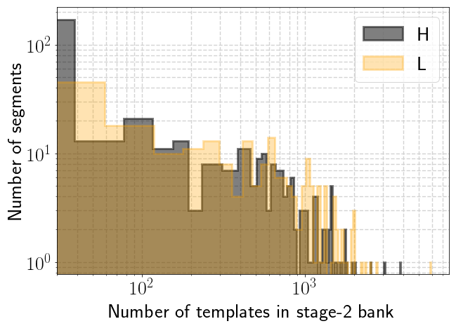
In the case of hierarchical search, the total number of matched-filter operations is the sum of the number of FFTs performed in stage 1 and stage 2. Since in stage-1 search we matched filter a data segment sampled at Hz using the coarse bank containing templates, the number of matched-filter operations becomes . If the same segment gets followed up to the stage-2 search, the number of matched-filter operations reduces due to fewer templates in a stage-2 bank. The number of templates in this bank can vary for each segment and detector, as can be seen from Fig. 11. Thus, we compute the total number of FFT operations for all the flat and combined stages of the hierarchical search segments. To estimate the overall gain in the computational speed, we take the ratio of the computed FFT operations for the flat to the hierarchical search.
We first define the following quantities:
| Quantity | Description |
| Total number of data segments in two detectors | |
| Duration of each segment | |
| Sampling rate for flat and stage-2 search | |
| Sampling rate for stage 1 | |
| Number of templates in the flat bank | |
| Number of templates in the stage-1 bank | |
| Total number of templates for all the segments | |
| used in the stage-2 search |
Let,
| (20) |
where and are the number of floating-point operations required to perform a FFT for a segment at the flat and coarse sampling rates, respectively. is a factor of few which cancels out from the numerator and denominator. Thus, the gain is given by
| (21) |
While the number of templates in flat search and stage 1 is fixed for all the segments, it varies for each segment in stage 2 as only specific triggers are followed up and filtered using a stage-2 bank. The total area of the histograms for the two detectors together shown in Fig. 11 provides us with . Since is much smaller than , the computation in stage 1 dominates the cost, so the stage-2 cost does not affect the gain.
Substituting the numerical values, and , the gain yielded is 22 for the analysis. We do not expect this number to change significantly for different observing runs. We also compare the actual CPU core hours used by the flat and hierarchical search for performing the matched-filtering operations. We found that the total CPU core hours used by the hierarchical search are around 824.16 and 547.37, respectively, for the Hanford and Livingston detectors. These numbers are nearly 1/19 times the number obtained for the flat search, i.e., 15,471.81 for Hanford and 10,478.64 for Livingston. Thus, we conclude that with the present setting, the hierarchical search provides an overall computational speed-up by a factor of .
V Conclusion and discussion
Efficient searches for GWs originating from CBCs can expand the size and dimensionality of the search parameter space to detect interesting sources with present and future detectors. The hierarchical search is perhaps the most straightforward approach that brings more than one order of magnitude enhancement in the efficiency without compromising the robustness of the search. In this work, we successfully demonstrate the efficiency of hierarchical search by applying the analysis on the first two observing runs of Advanced LIGO. By introducing essential modifications to the previously developed codes, we transform them into a complete analysis pipeline kan 2021. We improve the selection criteria for single-detector triggers using chi-square and sine-Gaussian vetoes to reweigh matched-filter SNRs. We also implement coincident detection statistics formulated in Nitz et al. 2017; Davies et al. 2020 in the hierarchical search that utilizes phase and time differences between detectors and detection parameters, significantly reducing false alarms due to noise events. With our pipeline, we recover all the events in the LIGO-Virgo Collaboration’s official transient catalog, GWTC-1, detected by the standard PyCBC analysis with nearly the same statistical confidence and a whopping factor of 20 computational speed-up. This work also demonstrates that hierarchical search is at hand for production analysis of the present and upcoming datasets from ground-based detectors.
Following Gadre et al. 2019, we estimate the detected candidates’ significance by scaling the noise background obtained in stage 1 with a factor close to the speed-up factor. Although the argument on assigning significance to detected candidates using this background may not be so rigorous, our work shows that this prescription works. The background estimation for the hierarchical search needs more scrutiny, and our future goal is to address this issue. It is outside the scope of the present investigation because an in-depth mathematical and statistical analysis of the empirical background estimation using time slides will be required. While the outcome of this exercise builds enough confidence for application in production runs that are otherwise restrictive due to computational cost, we plan to carry out an extensive study focused on accurate background estimation for the hierarchical search.
In our opinion, the hierarchical search pipeline can be used for ambitious searches that are currently deferred due to computational limitations. For instance, a search for binaries with nonaligned spins and subsolar sources requires an enormous number of templates. With hierarchical search, we can attempt to carry out their search at feasible computation cost without compromising the accuracy of sensitivity of the search. The hierarchical strategy could also reduce the computation cost of low-latency searches, which we plan to demonstrate in the future. Developing a comprehensive offline or a low-latency search for such sources is an arduous task ahead, and more sophisticated techniques will have to be brought in, in the coming years. Nevertheless, the hierarchical search is a major step in this direction that should be exploited.
Acknowledgements.
The authors acknowledge the computational resources provided by the IUCAA LDG cluster Sarathi, LIGO Laboratory, and are supported by National Science Foundation Grants. The authors acknowledge support from Soumen Roy in providing code and helping in the generation of banks. The authors are grateful for the valuable discussions from Shreejit P. Jadhav at various stages of this work. K. S. acknowledges technical support for cluster-related issues from Deepak Bankar. The hierarchical search pipeline uses PyCBC version 1.16.13 and is built upon LALSuite lal 2018, NumPy Walt et al. 2011, SciPy Virtanen et al. 2020, and Astropy Price-Whelan et al. 2018. K. S. acknowledges the Inter-University Centre of Astronomy and Astrophysics (IUCAA), India, for the fellowship support. B. G. acknowledges the support of the Max Planck Society. S. M. acknowledges support from the Department of Science and Technology (DST), Ministry of Science and Technology, India, provided under the Swarna Jayanti Fellowships scheme. S. V. D. acknowledges the support of the Senior Scientist Platinum Jubilee Fellowship from NASI, India. This manuscript has been assigned a LIGO Document No. LIGO-P2100202.References
- Abbott et al. (2016a) B. P. Abbott et al., Phys. Rev. Lett. 116, 061102 (2016a).
- Abbott et al. (2016b) B. P. Abbott et al., Phys. Rev. Lett. 116, 131103 (2016b).
- Abbott et al. (2016c) B. P. Abbott et al., Phys. Rev. D 93, 112004 (2016c).
- Klimenko et al. (2016) S. Klimenko, G. Vedovato, M. Drago, F. Salemi, V. Tiwari, G. A. Prodi, C. Lazzaro, K. Ackley, S. Tiwari, C. F. Da Silva, and G. Mitselmakher, Phys. Rev. D 93, 042004 (2016).
- Messick et al. (2017) C. Messick, K. Blackburn, P. Brady, P. Brockill, K. Cannon, R. Cariou, S. Caudill, S. J. Chamberlin, J. D. E. Creighton, R. Everett, et al., Phys. Rev. D 95, 042001 (2017).
- Usman et al. (2016) S. A. Usman, A. H. Nitz, I. W. Harry, C. M. Biwer, D. A. Brown, M. Cabero, C. D. Capano, T. D. Canton, T. Dent, S. Fairhurst, et al., Classical Quantum Gravity 33, 215004 (2016).
- Abbott et al. (2019a) B. P. Abbott et al., Phys. Rev. X 9, 031040 (2019a).
- Nitz et al. (2019) A. H. Nitz, C. Capano, A. B. Nielsen, S. Reyes, R. White, D. A. Brown, and B. Krishnan, Astrophys. J. 872, 195 (2019).
- Nitz et al. (2020) A. H. Nitz, T. Dent, G. S. Davies, S. Kumar, C. D. Capano, I. Harry, S. Mozzon, L. Nuttall, A. Lundgren, and M. Tápai, Astrophys. J. 891, 123 (2020).
- Venumadhav et al. (2019) T. Venumadhav, B. Zackay, J. Roulet, L. Dai, and M. Zaldarriaga, Phys. Rev. D 100, 023011 (2019).
- Aasi et al. (2015) J. Aasi, B. P. Abbott, R. Abbott, T. Abbott, M. R. Abernathy, K. Ackley, C. Adams, A. T., P. Addesso, et al., Classical Quantum Gravity 32, 074001 (2015).
- Acernese et al. (2014) F. Acernese, M. Agathos, K. Agatsuma, D. Aisa, N. Allemandou, A. Allocca, J. Amarni, P. Astone, G. Balestri, G. Ballardin, et al., Classical Quantum Gravity 32, 024001 (2014).
- Abbott et al. (2021a) R. Abbott et al., Phys. Rev. X 11, 021053 (2021a).
- Abbott et al. (2021b) R. Abbott et al., (2021b), arXiv:2108.01045 .
- Abbott et al. (2021c) R. Abbott et al., (2021c), arXiv:2111.03606 .
- Abbott et al. (2020a) B. P. Abbott et al., Astrophys. J. Lett. 892, L3 (2020a).
- Abbott et al. (2020b) B. P. Abbott et al., Phys. Rev. D 102, 043015 (2020b).
- Abbott et al. (2020c) R. Abbott et al., Astrophys. J. Lett. 896, L44 (2020c).
- Abbott et al. (2020d) R. Abbott et al., Astrophys. J. Lett. 900, L13 (2020d).
- Sathyaprakash and Dhurandhar (1991) B. S. Sathyaprakash and S. V. Dhurandhar, Phys. Rev. D 44, 3819 (1991).
- Dhurandhar and Sathyaprakash (1994) S. V. Dhurandhar and B. S. Sathyaprakash, Phys. Rev. D 49, 1707 (1994).
- Dhurandhar and Schutz (1994) S. V. Dhurandhar and B. F. Schutz, Phys. Rev. D 50, 2390 (1994).
- Owen and Sathyaprakash (1999) B. J. Owen and B. S. Sathyaprakash, Phys. Rev. D 60, 022002 (1999).
- Allen et al. (2012) B. Allen, W. G. Anderson, P. R. Brady, D. A. Brown, and J. D. E. Creighton, Phys. Rev. D 85, 122006 (2012).
- Sachdev et al. (2019) S. Sachdev, S. Caudill, H. Fong, K. L. R. Lo, C. Messick, D. Mukherjee, R. Magee, L. Tsukad, et al., (2019), arXiv:1901.08580 .
- Hanna et al. (2020) C. Hanna, C. Caudill, C. Messick, A. Reza, S. Sachdev, L. Tsukada, K. Cannon, K. Blackburn, J. D. E. Creighton, H. Fong, et al., Phys. Rev. D 101, 022003 (2020).
- Adams et al. (2016) T. Adams, D. Buskulic, V. Germain, G. M. Guidi, F. Marion, M. Montani, B. Mours, F. Piergiovanni, and G. Wang, Classical Quantum Gravity 33, 175012 (2016).
- Aubin et al. (2021) F. Aubin, F. adn Brighenti, R. Chierici, D. Estevez, G. Greco, G. M. Guidi, J. V., F. Marion, B. Mours, E. Nitoglia, et al., Classical Quantum Gravity 38, 095004 (2021).
- Davies et al. (2020) G. S. Davies, T. Dent, M. Tápai, I. Harry, C. McIsaac, and A. H. Nitz, Phys. Rev. D 102, 022004 (2020).
- Chu (2017) Q. Chu, Ph.D. thesis, The University of Western Australia (2017).
- Canton and W. (2017) T. D. Canton and H. I. W., (2017), arXiv:1705.01845 .
- Harry et al. (2016) I. Harry, S. Privitera, A. Bohé, and A. Buonanno, Phys. Rev. D 94, 024012 (2016).
- Abbott et al. (2019b) B. P. Abbott et al., Phys. Rev. Lett. 123, 161102 (2019b).
- Abbott et al. (2021d) R. Abbott et al., (2021d), arXiv:2109.12197 .
- Nitz and Wang (2021) A. H. Nitz and Y.-F. Wang, Astrophys. J. 915, 54 (2021).
- Akutsu et al. (2020) T. Akutsu, M. Ando, K. Arai, Y. Arai, S. Araki, S. Araya, N. Aritomi, Y. Aso, S. Bae, Y. Bae, et al., (2020), arXiv:2005.05574 .
- Iyer et al. (2011) B. Iyer et al., LIGO-India Tech. rep. (2011).
- Mohanty and Dhurandhar (1996) S. D. Mohanty and S. V. Dhurandhar, Phys. Rev. D 54, 7108 (1996).
- Mohanty (1998) S. D. Mohanty, Phys. Rev. D 57, 630 (1998).
- Gadre et al. (2019) B. Gadre, S. Mitra, and S. Dhurandhar, Phys. Rev. D 99, 124035 (2019).
- Devine et al. (2016) C. Devine, Z. B. Etienne, and S. T. McWilliams, Classical Quantum Gravity 33, 125025 (2016).
- Prix (2007) R. Prix, Classical Quantum Gravity 24, S481 (2007).
- Harry et al. (2009) I. W. Harry, B. Allen, and B. S. Sathyaprakash, Phys. Rev. D 80, 104014 (2009).
- Roy et al. (2017) S. Roy, A. S. Sengupta, and N. Thakor, Phys. Rev. D 95, 104045 (2017).
- Roy et al. (2019) S. Roy, A. S. Sengupta, and P. Ajith, Phys. Rev. D 99, 024048 (2019).
- Harry and Fairhurst (2011) I. W. Harry and S. Fairhurst, Phys. Rev. D 83, 084002 (2011).
- Keppel (2013a) D. Keppel, Phys. Rev. D 87, 124003 (2013a).
- Keppel (2013b) D. Keppel, (2013b), arXiv:1307.4158 .
- Buonanno et al. (2003) A. Buonanno, Y. Chen, and M. Vallisneri, Phys. Rev. D 67, 104025 (2003).
- Kalaghatgi et al. (2015) C. Kalaghatgi, P. Ajith, and K. G. Arun, Phys. Rev. D 91, 124042 (2015).
- Sengupta et al. (2002) A. S. Sengupta, S. V. Dhurandhar, A. Lazzarini, and T. Prince, Classical Quantum Gravity 19, 1507 (2002).
- Abbott et al. (2016d) B. P. Abbott et al., Classical Quantum Gravity 33, 134001 (2016d).
- Zevin et al. (2017) M. Zevin, S. Coughlin, S. Bahaadini, E. Besler, N. Rohani, S. Allen, M. Cabero, K. Crowston, A. K. Katsaggelos, S. L. Larson, et al., Classical Quantum Gravity 34, 064003 (2017).
- Huang et al. (2018) Y. Huang, H. Middleton, K. K. Y. Ng, S. Vitale, and J. Veitch, Phys. Rev. D 98, 123021 (2018).
- Abbott et al. (2018) B. P. Abbott et al., Classical Quantum Gravity 35, 065010 (2018).
- Allen et al. (1999) B. Allen, J. K. Blackburn, P. R. Brady, J. D. E. Creighton, T. Creighton, S. Droz, A. D. Gillespie, S. A. Hughes, S. Kawamura, T. T. Lyons, et al., Phys. Rev. Lett. 83, 1498 (1999).
- Nitz (2018) A. H. Nitz, Classical Quantum Gravity 35, 035016 (2018).
- Nitz et al. (2017) A. H. Nitz, T. Dent, T. D. Canton, S. Fairhurst, and D. A. Brown, Astrophys. J. 849, 118 (2017).
- Biswas et al. (2012) R. Biswas, P. R. Brady, J. Burguet-Castell, K. Cannon, J. Clayton, A. Dietz, N. Fotopoulos, L. M. Goggin, D. Keppel, C. Pankow, L. R. Price, and R. Vaulin, Phys. Rev. D 85, 122008 (2012).
- kan (2021) Hierarchical search pipeline, https://github.com/Kanchan-05/pycbc/tree/Hierarchical-search/hierarchical_search (2021).
- Tiwari (2018) V. Tiwari, Classical Quantum Gravity 35, 145009 (2018).
- Sturani et al. (2010) R. Sturani, S. Fischetti, L. Cadonati, G. M. Guidi, J. Healy, D. Shoemaker, and A. Viceré, Journal of Physics: Conference Series 243, 012007 (2010).
- lal (2018) Ligo scientific collaboration, ligo algorithm library— lalsuite, free software (gpl) (2018).
- Walt et al. (2011) S. v. d. Walt, S. C. Colbert, and G. Varoquaux, Comput. Sci. Eng. 13 (2011).
- Virtanen et al. (2020) P. Virtanen et al., Nat. Methods 17 (2020).
- Price-Whelan et al. (2018) A. M. Price-Whelan et al., Astron. J. 156 (2018).
*