Axion clouds may survive the perturbative tidal interaction over the early inspiral phase of black hole binaries

Rotating BHs are described by the Kerr spacetime. Consider a real scalar field (axion) $\phi$ of mass $\mu$ on the Kerr metric $g_{\mu\nu}$, which is characterized by the mass $M$ and the angular momentum $J=aM$ of the BH. The equation of motion of a scalar field is

$$\left(g^{\mu\nu}\nabla_{\mu}\nabla_{\nu}-\mu^{2}\right)\phi(x)=0\quad.$$

(2.1)

Solutions of this equation can be obtained in the form of [19]

$$\phi(x)={\rm{Re}}\left[e^{-i(\omega t-m\varphi)}S_{lm\omega}(\theta)R_{lm\omega}(r)\right]\quad,$$

(2.2)

where $l,m$ are the labels of the spheroidal harmonics $e^{im\varphi}S_{lm\omega}(\theta)$. Owing to the mass of the scalar field, this system admits quasi-bound state solutions that vanish at the spatial infinity and are purely ingoing waves at the BH horizon. Under these boundary conditions, there exist solutions corresponding to infinitely many, discrete eigenfrequencies, which are complex because of the energy transfer through the horizon. Thus, we denote eigenfrequencies as

$$\omega_{nlm}=(\omega_{R})_{nlm}+i(\omega_{I})_{nlm}\quad,$$

(2.3)

where $n>0$ denotes the order of the overtone. Without loss of generality, we can assume $(\omega_{R})_{nlm}>0$. For modes satisfying the superradiance conditions ¹¹ 1 Strictly speaking, for complex $\omega$, the superradiance condition becomes $|\omega|^{2}/\omega_{R}<m\Omega_{H}$ [6], but the imaginary part of the eigenfrequencies of bound states is always very small compared to the real part.

$$\omega_{R}<m\Omega_{H}\quad,$$

(2.4)

and $\omega_{I}$ becomes positive, where $\Omega_{H}:=a/2Mr_{+}$ is the angular velocity of the BH horizon and $r_{+}=M+\sqrt{M^{2}-a^{2}}$ is the horizon radius. This positive imaginary part of the frequency means that a gravitationally bound scalar field continues to grow to form a heavy cloud extracting the energy and the angular momentum from the BH.

In the non-relativistic limit, it is appropriate to start with the ansatz

$$\phi(t,\bm{r})=\frac{1}{\sqrt{2\mu}}\left[\psi(t,\bm{r})e^{-i\mu t}+{\rm{c.c.}}\right]\quad,$$

(2.5)

and $\psi(t,\bm{r})$ is a complex scalar function that slowly varies on time scales much longer than $\mu^{-1}$. Substituting Eq. (2.5) into Eq. (2.1), and keeping only the leading order terms in $r^{-1}$, we obtain

$$i\frac{\partial}{\partial t}\psi=\left(-\frac{1}{2\mu}\nabla^{2}-\frac{M\mu}{r}\right)\psi\quad.$$

(2.6)

This equation is formally equivalent to the Schr${\rm{\ddot{o}}}$dinger equation for a hydrogen atom. For smaller $M\mu$, the radius of the cloud is larger, and hence the effect of the presence of the horizon is weaker. In the non-relativistic limit the eigenfunctions $\psi_{nlm}$ are reduced to the ones for a hydrogen atom, and the eigenfrequencies can be given by

$$(\omega_{R})_{nlm}=\mu\left(1-\frac{(M\mu)^{2}}{2n^{2}}+\Delta\omega_{nlm}\right)\quad,$$

(2.7)

where $\Delta\omega_{nlm}$ represents higher-order corrections in $M\mu$, whose approximate expression is given in Ref. [13]. For example, this correction breaks the degeneracies between modes with the same $n$ and $l$ but with different $m$ by an order of $(M\mu)^{5}$. Note that the labels of eigenstates that we can take are restricted to $n>0,l\leq n-1,|m|\leq l$. Approximate formulas for the imaginary part $(\omega_{I})_{nlm}$ are given by Detweiler [20].

Following Ref. [14], we review what happens when a BH with an axion cloud forms a binary system. The tidal perturbation from the binary companion can be described by an additional potential $V_{*}(t)$ in Eq. (2.6). We denote the eigenstates of the axion cloud as $\ket{i}$, and a general bound state can be written by a superposition of eigenstates, i.e., $\displaystyle\ket{\psi(t)}=\sum_{i}c_{i}(t)\ket{i}$. As in the case of quantum mechanics, $|c_{i}(t)|^{2}$ represents the occupation number, and its time evolution is given by

$$i\frac{\mathrm{d}c_{i}}{\mathrm{d}t}=\sum_{j}\mathcal{H}_{ij}(t)c_{j}=\sum_{j}\left[\omega_{i}\delta_{ij}+V_{ij}(t)\right]c_{j}\quad,$$

(2.8)

where $V_{ij}=\braket{i|V_{*}|j}$ encapsulates the effect of tidal perturbation from the binary companion. For simplicity, let us assume that the binary orbit is of a large radius, quasi-circular and on the plane perpendicular to the BH spin. We can write the perturbation as

$$V_{ij}=\eta_{ij}\exp\left(-i\Delta m_{ij}\int_{0}^{t}dt^{\prime}\Omega(t^{\prime})\right)\quad,$$

(2.9)

where $\eta_{ij}$ represents the amplitude of the perturbation, $\Delta m_{ij}=m_{i}-m_{j}$ and $\Omega(t)$ is the orbital angular velocity. There are selection rules, i.e., the conditions that $\eta_{ij}$ does not vanish. We summarize the selection rules with the explicit expression of tidal perturbation in appendix A. If the time variation of orbital angular velocity is sufficiently slow, as is well known from the time-dependent perturbation theory in quantum mechanics, a resonant level transition occurs when the orbital angular velocity coincides with the gap of phase velocities of two levels. Thus, we define the resonance frequency as

$$\pm\Omega_{\mathrm{res}}=\frac{\Delta E_{ij}}{\Delta m_{ij}}\quad,$$

(2.10)

where $\Delta E_{ij}=(\omega_{R})_{i}-(\omega_{R})_{j}$ and the upper (lower) sign denotes the case of co-rotating (counter-rotating) orbits. In particular, if the time dependence of the orbital angular velocity is approximated by a linear function as

$$\Omega(t)=\Omega_{\mathrm{res}}+\gamma_{ij}t\quad,$$

(2.11)

the problem to solve is known as the Landau-Zener transition. For example, consider a two-level system with an initial condition with $c_{1}(-\infty)=1$ and $c_{2}(-\infty)=0$. A resonant transition occurs at around $t=0$ (resonance frequency), and the occupation number at a late time is given by

$$|c_{1}(+\infty)|^{2}=e^{-2\pi z}\ ,\quad|c_{2}(+\infty)|^{2}=1-e^{-2\pi z}\quad,$$

(2.12)

where $z\equiv\eta_{ij}^{2}/|\Delta m_{ij}|\gamma_{ij}$. Intuitively, this quantity $z$ roughly measures whether the transition timescale $\Delta t\sim 2\eta/\gamma$ is long enough in passing thorough the resonance band $\Delta\Omega\sim 2\eta$. If $z\gg 1$, the transition is adiabatic and almost all axions are transferred to the other mode.

For the inspiral phase of a binary, $\eta_{ij}$ and $\gamma_{ij}$ are given by

	$\displaystyle\frac{\eta_{ij}}{\Omega_{\mathrm{res}}}$	$\displaystyle\simeq 0.3\left(\frac{R_{ij}}{0.3}\right)\frac{q}{1+q}\quad,$		(2.13)
	$\displaystyle\frac{\gamma_{ij}}{\Omega^{2}_{\mathrm{res}}}$	$\displaystyle\simeq 8.0\times 10^{-6}\frac{q}{(1+q)^{1/3}}\left(\frac{M}{30M_{\odot}}\right)^{5/3}\left(\frac{\Omega_{\mathrm{res}}}{1\mathrm{Hz}}\right)^{5/3}\quad,$		(2.14)

where we have defined the mass ratio $q\equiv M_{*}/M$ with $M_{*}$ being the mass of the binary companion. $R_{ij}$ characterizes the overlap of different two bound states and typically $R_{ij}\lesssim 0.3$. For small $M\mu$, the fastest growing mode is $\ket{211}$ and the axion cloud is dominated by this mode. Since the orbital angular velocity gradually increases, the transition occurs first between the levels with the lowest resonance frequencies. From the selection rules, only transitions with $\Delta l=2p~(p\in\mathbb{Z})$ and $|\Delta m|=2$ are possible for equatorial orbits. In this case, the growing mode $\ket{211}$ makes a transition to a decaying mode $\ket{21-1}$ ($\ket{31-1}$) for co-rotating (counter-rotating) orbits. The resonance frequencies can be calculated by Eq. (2.7), and $\Omega_{\mathrm{res}}\simeq 2.3\times 10^{-4}\mathrm{Hz}~(30M_{\odot}/M)(M\mu/0.1)^{7}$ ($0.24\mathrm{Hz}~(30M_{\odot}/M)(M\mu/0.1)^{3}$). Therefore, if $q=\mathcal{O}(1)$, $z\gg 1$ is satisfied by inspiral orbits and transitions should be adiabatic. As a result, the axion clouds disappear in the early inspiral phase.

We investigate to which mode the first transition occurs depending on the binary parameters when $l=1,2$ or $3$ is the fastest growing mode. For $l\geq 4$ mode, the growth rate is suppressed and it may not be so interesting in a realistic situation. Which transition first occurs is determined by evaluating the energy gaps between the growing mode of interest and the other modes. We calculate the eigenfrequencies of all relevant modes allowed for the transitions numerically using the continued fraction method (see appendix B). They depend on two parameters $(M\mu,a/M)$. As a realistic maximum value of a spin parameter, we adopt the Thorne limit $a/M=0.998$ [21]. We show the energy spectra of relevant modes as a function of $M\mu$ for the maximum value of spin for each $l$ in figure. 1 as an example.

From these figures, we can see that, because of the non-trivial behavior of energy levels, it is not possible to guess which transition occurs from the analogy of the hydrogen atom and it depends on the parameters. Comparing the energy differences from the focused growing mode, we classified the parameter space based on the destination of the first transition. The transition destination changes where the crossing between the relevant energy levels occurs. We made the map that shows the transition destination in the parameter plane as shown in figure. 2. As a first step, we consider only quadrupolar tidal perturbation. For simplicity, we focus on the case in which the binary orbit is on the equatorial plane, i.e., only the transitions with $|\Delta m|=2$ are allowed. However, as we will see later, the conclusion will be unaltered even if we consider more general orbits, except for the case of an extremely large BH spin.

For $l=1$, level crossing between relevant modes does not occur in the superradiant region ²² 2 $(\omega_{R})_{211}$ and $(\omega_{R})_{21-1}$ coincide at $M\mu=4.97$, and the condition $(\omega_{R})_{211}<\Omega_{H}$ is violated at $M\mu=0.489$ for $a/M=0.998$., and hence the transition destinations are the same as the non-relativistic limit, i.e., $\ket{211}\to\ket{21-1}$ for the co-rotating case and $\ket{211}\to\ket{31-1}$ for the counter-rotating case. For $l=2$, as shown in figure. 2, the transition destination depends on the values of parameters, but in almost the whole region, axions are transferred to a decaying mode which has the value of $m$ smaller than the original one. As an exception, in the co-rotating case, axions make a transition to the growing mode $\ket{544}$ in the region with a very large BH spin. However, in the presence of the superradiance, such a very large spin may not be realistic, since the process of the axion cloud formation extracts the angular momentum of the BH. For $l=3$, we should note that the growing mode with $n\neq l+1$ can be the fastest. Therefore, for each region where $n=4,5$ or $6$ is the fastest growing mode, we made a separate map showing the first transition destination. Similar to $l=2$, axions make a transition to a decaying mode in the almost whole region except for the region with a very large BH spin.

If the binary orbit is inclined, the transitions with $|\Delta m|=1$ are also allowed. Then, for example, $\ket{322}$ is first transferred to $\ket{321}$ in a wide parameter region for the co-rotating case. However, this means $(\omega_{R})_{322}-(\omega_{R})_{321}<(\omega_{R})_{321}-(\omega_{R})_{320}$, and hence the next transition $\ket{321}\to\ket{320}$ will occur successively. Therefore, the results described below should be almost unaltered. Furthermore, for the region with a very large BH spin where the transition to a growing mode occurs in the case of equatorial orbits, the transition to a decaying mode with $m$ less than one can occur in the non-equatorial case. On the other hand, in the counter-rotating case, the first transition destination will not change even if the orbit is inclined.

Now that we know which transition occurs for each set of parameters, we can evaluate how much fraction of the cloud disappears between the first transition and the coalescence. Since the adiabatic condition of the transition is satisfied during the inspiral phase, we assume all axions are transferred to another mode at the resonance frequency immediately after crossing the resonance frequency. Then, we can estimate the mass of axion clouds after transition as ³³ 3 As mentioned in Ref. [14], the estimation of the total amount of depletion in Ref. [13, 15] assumes a constant orbital frequency. Therefore, they are not appropriate for the situation that we are considering.

$$M_{cl}(t)\simeq M_{0}\exp\left[2(\omega_{I})t_{m}\right]\quad,$$

(3.1)

where $M_{0}$ is the initial mass of axion clouds at the resonance frequency and $\omega_{I}$ is the imaginary part of the eigenfrequency of the transition destination. For quasi-circular orbits, the merger time taken from the resonance frequency to the coalescence is [22]

$$t_{m}=\frac{5}{256}\frac{(1+q)^{1/3}}{q}(M\Omega_{\mathrm{res}})^{-8/3}M\quad.$$

(3.2)

To see whether or not axion clouds survive until around the merger phase, we should evaluate $|(\omega_{I})_{i}|t_{m}$, where $i$ is the label of the mode of transition destination for each parameter region shown in figure. 2. In particular, since we focus on the observability of axion clouds with ground-based detectors, we consider the case with $q=1$. We show the numerical estimate about how a large fraction of the cloud mass disappears considering only the first transition in figure. 3.

For $l=1$, in the co-rotating case, $|\omega_{I}|_{i}t_{m}$ is very large in the whole region. This means that the resonance frequency is so small, and the time before the coalescence is so long that there is a sufficiently long time for the clouds to disappear. Conversely, in the counter-rotating case, $|\omega_{I}|_{i}t_{m}$ is small, especially in the non-relativistic regime. This is because the resonance frequency is large in the counter-rotating case, and the time before the coalescence is short. However, for the relativistic regime, the decay rate is large, and hence $|\omega_{I}|_{i}t_{m}$ becomes large enough for the clouds to disappear.

For $l=2$, in the co-rotating case, $|\omega_{I}|_{i}t_{m}$ is very large in the whole region as in $l=1$ case. Also, in the counter-rotating case, $|\omega_{I}|_{i}t_{m}$ is very large in the whole region unlike in the $l=1$ case. Axions occupying the $l=2$ growing mode make a transition to the mode whose value of $l$ is smaller than the original one and its decay rate is very large because of the lower angular momentum barrier. Therefore, even with a short time before coalescence, the clouds almost disappear. Such transitions are absent in the $l=1$ case owing to the selection rule.

For $l=3$, in the region where transition destination is $\ket{n31}(n=4,5,6)$ except for the region with a large $M\mu$, $|\omega_{I}|_{i}t_{m}$ is small because the decay rate of $\ket{n31}$ is so small. In the other region of interest, $|\omega_{I}|_{i}t_{m}$ is so large that the clouds almost disappear.

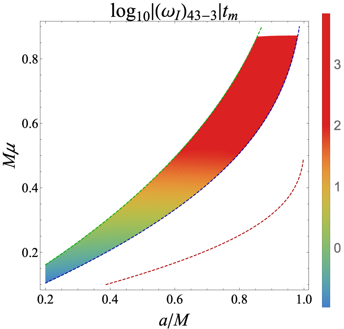
As seen in figure. 3, there are parameter regions where the clouds do not disappear if we consider only the first transition. To conclude whether the clouds in such parameter regions disappear or not, we need to investigate the subsequent transitions, too.

For the $l=1$ counter-rotating case, axions are first transferred to $\ket{31-1}$. Since transitions occur only when $\Delta E/\Delta m<0$ and there is no mode with $l\geq 1$ at energy levels lower than $\ket{31-1}$, axions will be next transferred to higher energy mode. Considering the orbits on the equatorial plane, i.e., allowing only transitions with $|\Delta m|=2$, because $(\omega_{R})_{31-1}-(\omega_{R})_{21-1}>\mu-(\omega_{R})_{31-1}$, the next transition will not occur. In the non-equatorial orbit case, axions can be next transferred to higher-$l$ mode, e.g. $\ket{53-2}$. However, they have a very small decay rate. Therefore, the cloud will not disappear at least when we take into account only the quadrupolar tidal perturbation.

For the $l=3$ co-rotating case, considering the transition $\ket{433}\to\ket{431}$, successive transitions $\ket{431}\to\ket{43-1}\to\ket{43-3}$ will occur. Hence, we should judge whether the clouds disappear or not by evaluating $|(\omega_{I})_{43-3}|t_{m}$. The result is shown in figure. 4 and it is large at $M\mu\gtrsim 0.3$. Notice that the original growth rate of higher-$l$ mode is suppressed by the higher angular momentum barrier and there is less physical interest in the small $M\mu$ region for $l=3$. A similar thing happens to $n=5$. In the counter-rotating case, axions that experience the transition to $\ket{531}$ or $\ket{631}$ will then be transferred to the mode with $m=-1$. Its decay rate should be very large and the clouds disappear.

References

- [1] LIGO Scientific, Virgo collaboration, Observation of Gravitational Waves from a Binary Black Hole Merger, Phys. Rev. Lett. 116 (2016) 061102 [1602.03837].
- [2] LIGO Scientific, Virgo collaboration, GW150914: First results from the search for binary black hole coalescence with Advanced LIGO, Phys. Rev. D 93 (2016) 122003 [1602.03839].
- [3] LIGO Scientific, Virgo collaboration, GWTC-2: Compact Binary Coalescences Observed by LIGO and Virgo During the First Half of the Third Observing Run, 2010.14527.
- [4] A. Arvanitaki, S. Dimopoulos, S. Dubovsky, N. Kaloper and J. March-Russell, String Axiverse, Phys. Rev. D81 (2010) 123530 [0905.4720].
- [5] R. Brito, V. Cardoso and P. Pani, Superradiance, Lect. Notes Phys. 971 (2020) pp.1 [1501.06570].
- [6] S.R. Dolan, Instability of the massive Klein-Gordon field on the Kerr spacetime, Phys. Rev. D76 (2007) 084001 [0705.2880].
- [7] A. Arvanitaki and S. Dubovsky, Exploring the String Axiverse with Precision Black Hole Physics, Phys. Rev. D83 (2011) 044026 [1004.3558].
- [8] A. Arvanitaki, M. Baryakhtar and X. Huang, Discovering the QCD Axion with Black Holes and Gravitational Waves, Phys. Rev. D91 (2015) 084011 [1411.2263].
- [9] A. Arvanitaki, M. Baryakhtar, S. Dimopoulos, S. Dubovsky and R. Lasenby, Black Hole Mergers and the QCD Axion at Advanced LIGO, Phys. Rev. D 95 (2017) 043001 [1604.03958].
- [10] H. Yoshino and H. Kodama, Gravitational radiation from an axion cloud around a black hole: Superradiant phase, PTEP 2014 (2014) 043E02 [1312.2326].
- [11] R. Brito, V. Cardoso and P. Pani, Black holes as particle detectors: evolution of superradiant instabilities, Class. Quant. Grav. 32 (2015) 134001 [1411.0686].
- [12] R. Brito, S. Ghosh, E. Barausse, E. Berti, V. Cardoso, I. Dvorkin et al., Gravitational wave searches for ultralight bosons with LIGO and LISA, Phys. Rev. D96 (2017) 064050 [1706.06311].
- [13] D. Baumann, H.S. Chia and R.A. Porto, Probing Ultralight Bosons with Binary Black Holes, Phys. Rev. D 99 (2019) 044001 [1804.03208].
- [14] D. Baumann, H.S. Chia, R.A. Porto and J. Stout, Gravitational Collider Physics, Phys. Rev. D 101 (2020) 083019 [1912.04932].
- [15] E. Berti, R. Brito, C.F.B. Macedo, G. Raposo and J.L. Rosa, Ultralight boson cloud depletion in binary systems, Phys. Rev. D 99 (2019) 104039 [1904.03131].
- [16] S. Choudhary, N. Sanchis-Gual, A. Gupta, J.C. Degollado, S. Bose and J.A. Font, Gravitational waves from binary black hole mergers surrounded by scalar field clouds: Numerical simulations and observational implications, Phys. Rev. D 103 (2021) 044032 [2010.00935].
- [17] M. Baryakhtar, M. Galanis, R. Lasenby and O. Simon, Black hole superradiance of self-interacting scalar fields, Phys. Rev. D 103 (2021) 095019 [2011.11646].
- [18] H. Omiya, T. Takahashi and T. Tanaka, Renormalization group analysis of superradiant growth of self-interacting axion cloud, PTEP 2021 (2021) 043E02 [2012.03473].
- [19] D.R. Brill, P.L. Chrzanowski, C.M. Pereira, E.D. Fackerell and J.R. Ipser, Solution of the Scalar Wave Equation in a Kerr Background by Separation of Variables, Phys. Rev. D5 (1972) 1913.
- [20] S.L. Detweiler, KLEIN-GORDON EQUATION AND ROTATING BLACK HOLES, Phys. Rev. D22 (1980) 2323.
- [21] K.S. Thorne, Disk accretion onto a black hole. 2. Evolution of the hole., Astrophys. J. 191 (1974) 507.
- [22] P.C. Peters, Gravitational radiation and the motion of two point masses, Phys. Rev. 136 (1964) B1224.
- [23] E.W. Leaver, Solutions to a generalized spheroidal wave equation: Teukolsky’s equations in general relativity, and the two-center problem in molecular quantum mechanics, Journal of Mathematical Physics 27 (1986) 1238 [https://doi.org/10.1063/1.527130].
- [24] E. Berti, V. Cardoso and M. Casals, Eigenvalues and eigenfunctions of spin-weighted spheroidal harmonics in four and higher dimensions, Phys. Rev. D73 (2006) 024013 [gr-qc/0511111].