Learning Algorithms for Markovian Bandits:
Is Posterior Sampling more Scalable than Optimism?
Abstract
In this paper, we study the scalability of model-based algorithms learning the optimal policy of a discounted Markovian bandit problem with arms. There are two categories of model-based reinforcement learning algorithms: Bayesian algorithms (like PSRL), and optimistic algorithms (like UCRL2 or UCBVI). While a naïve application of these algorithms is not scalable because the state-space is exponential in , we construct variants specially tailored to Markovian bandits (MB) that we call MB-PSRL, MB-UCRL2, and MB-UCBVI. They all have a low regret in – where is the number of episodes, is the number of arms and is the number of states of each arm. Up to a factor , these regrets match the lower bound of that we also derive.
Even if their theoretical regrets are comparable, the practical applicability of those algorithms varies greatly: We show that MB-UCRL2, as well as all algorithms that use bonus on transition matrices, cannot be implemented efficiently (its time complexity is exponential in ). As MB-UCBVI does not use bonus on transition matrices, it can be implemented efficiently but our numerical experiments show that its empirical regret is large. Our Bayesian algorithm, MB-PSRL takes the best of both worlds: its running time is linear in the number of arms and its empirical regret is the smallest of all algorithms. This shows the power of Bayesian algorithms, that can often be easily tailored to the structure of the problems to learn.
Keywords:
Reinforcement Learning, Posterior Sampling, Gittins index, Rested bandit, Bayesian approach, Optimistic approach1 Introduction
Markov Decision Processes (MDPs) are a powerful model to solve stochastic optimization problems. They suffer, however, from what is called the curse of dimensionality: the state size of a Markov process is exponential in its number of dimensions, so that the complexity of computing an optimal policy is exponential in the number of dimensions of the problem. The same holds for general purpose reinforcement learning algorithm: they all have a regret and a runtime exponential in the number of dimensions, so they also suffer from the same curse. Very few MDPs are known to escape from this curse of dimensionality. One of the most famous examples is the Markovian bandit problem for which an optimal policy and its value can be computed in , where is the number of arms: The optimal policy can be computed by using the Gittins indices (computed locally) and its value can be computed by using retirement values (see for example [41]).
In this paper, we study a specialization of PSRL [28] to Markovian bandits, that we call Markovian bandit posterior sampling (MB-PSRL) that consists in using PSRL with a prior tailored to Markovian bandits. We show that the regret of MB-PSRL is sub-linear in the number of episodes and of arms. We also provide a regret guarantee for two optimistic algorithms that we call MB-UCRL2 and MB-UCBVI, and that are based respectively on UCRL2 [22] and UCBVI [4]. They both use modified confidence bounds adapted to Markovian bandit problems. The upper bound for their regret is similar to the bound for MB-PSRL. This shows that in terms of regret, the posterior sampling approach (MB-PSRL) and the optimistic approach (MB-UCRL2 and MB-UCBVI) scale well with the number of arms. We also provide a lower bound on the regret of any learning algorithm in Markovian bandit problems, which shows that the regret bounds that we obtain for all algorithms are close to optimal.
The situation is radically different when considering the processing time: the runtime of MB-PSRL is linear in the number of arms, while the runtime of MB-UCRL2 is exponential in . We show that this is not an artifact of our implementation of MB-UCRL2 by exhibiting a Markovian bandit problem for which being optimistic in each arm is not optimistic in the global MDP. This implies that UCRL2 and its variants [6, 14, 35, 10] cannot be adapted to have linear runtime in Markovian bandit problem unless an oracle is given. We argue that this non-scalability of UCRL2 and variants is not a property of optimistic approach but comes from the fact that UCRL2 relies on extended value iteration [22] needed to deal with upper confidence bounds on the transition matrices. We show that MB-UCBVI, an optimistic algorithm that does not add bonus on transition probabilities and hence does not rely on extended value iteration, does not suffer from the same problem. Its regret is sub-linear in the number of episodes, arms, and states per arm (although larger than the regret of both MB-PSRL and MB-UCRL2), and its runtime is linear in the number of arms.
We conduct a series of numerical experiments to compare the performance of MB-PSRL, MB-UCRL2 and MB-UCBVI. They confirm the good behavior of MB-PSRL, both in terms of regret and computational complexity. These numerical experiments also show that the empirical regret of MB-UCBVI is larger than the regret of MB-PSRL and MB-UCRL2, confirming the comparisons between the upper bounds derived in Theorem 5.1. All this makes MB-PSRL the better choice between the three learning algorithms.
Related Work
We focus on Markovian bandit problem with discount factor and all reward functions and transition matrices are unknown. A possible approach to learn such a problem is to ignore the problem structure and view the Markovian bandit problem as a generic MDP. There are two main families of generic reinforcement learning algorithms with regret guarantees. The first one uses the optimism in face of uncertainty (OFU) principle. OFU methods build a confidence set for the unknown MDP and compute an optimal policy of the “best” MDP in the confidence set, e.g., [6, 13, 4, 22, 5]. UCRL2 [22] is a well known OFU algorithm. The second family uses a Bayesian approach, the posterior sampling method introduced in [36]. Such algorithms keep a posterior distribution over possible MDPs and execute the optimal policy of a sampled MDP, see e.g., [30, 1, 19, 28]. PSRL is a classical example of Bayesian learning algorithm. All these algorithms, based on OFU or on Bayesian principles, have sub-linear bounds on the regret, which means that they provably learn the optimal policy. Yet, applied as-is to Markovian bandit problems, these bounds grow exponentially with the number of arms.
Our work is not the first attempt to exploit the structure of a MDP to improve learning. Factored MDPs (the state space can be factored into components) are investigated in [20], where asymptotic convergence to the optimal policy is proved to scale polynomially in the number of components. The regret of learning algorithms in factored MDP with a factored action space is considered in [37, 33, 42, 26]. Our work differs substantially from these. First, the Markovian bandit problem is not a factored MDP because the action space is global and cannot be factored. Second, our reward is discounted over an infinite horizon while factored MDPs have been analyzed with no discount. Finally, and most importantly, the factored MDP framework assumes that the successive optimal policies are computed by an unspecified solver. There is no guarantee that the time complexity of this solver scales linearly with the number of components, especially for OFU-based algorithms. For Markovian bandits, we get an additional leverage: when all parameters are known, the Gittins index policy is known to be an optimal policy and its computational complexity is linear in the number of arms. This reveals an interesting difference between Bayesian and extented value based algorithms (the former being scalable and not the latter), which is not present in the literature about factored MDPs because such papers do not consider the time complexity.
Since index policies scale with the number of arms, using Q-learning approaches to learn such a policy is also popular e.g., [3, 15, 9]. The authors of [9] address the same Markovian bandit problem as we do: their algorithm learns the optimal value in the restart-in-state MDP [24] for each arm and uses Softmax exploration to solve the exploration-exploitation dilemma. As mentioned on page in [2], however, there exists no finite-time regret bounds for this algorithm. Furthermore, tuning its hyperparameters (learning rate and temperature) is rather delicate and unstable in practice.
2 Markovian Bandit Problem
In this section, we introduce the Markovian bandit problem and recall the notion of Gittins index when the parameters of all arms are known.
2.1 Definitions and Main Notations
We consider a Markovian bandit problem with arms. Each arm for is a Markov reward process with a finite state space of size . Each arm has a mean reward vector, , and a transition matrix . When Arm is activated in state , it moves to state with probability . This provides a reward whose expected value is . Without loss of generality, we assume that the state spaces of the arms are pairwise distinct: for . In the following, the state of an arm will always be denoted with an index : we will denote such a state by or . As state spaces are disjoint, this allows us to simplify the notation by dropping the index from the reward and transition matrix: when convenient, we will denote them by instead of and by instead of since no confusion is possible.
At time , the global state is distributed according to some initial distribution over the global state space . At time , the decision maker observes the states11 1 Throughout the paper, we use capital letters (like ) to denote random variables and small letter (like ) to denote their realizations. Bold letters ( or ) design vectors. Normal letters ( or ) are for scalar values. of all arms, , and chooses which arm to activate. This problem can be cast as a MDP – that we denote by – with state space and action space . Let and . If the state at time is , the chosen arm is , then the agent receives a random reward drawn from some distribution on with mean and the MDP transitions to state with probability that satisfies:
That is, the active arm makes a transition while the other arms remain in the same state.
Let be the set of deterministic policies, i.e., the set of functions . For the MDP , we denote by the expected cumulative discounted reward of under policy starting from an initial state :
An alternative definition of is to consider a finite-horizon problem with a geometrically distributed length. Indeed, let be a time-horizon geometrically distributed with parameter . We have
| (3) |
Problem 1
Given a Markovian bandit with arms, each is a Markov reward process with a finite state space of size , find a policy that maximizes for any state distributed according to initial global state distribution .
2.2 Gittins Index Policy
It is possible to compute an optimal policy for Problem 1 in a reasonable amount of time using the so called Gittins indices: Gittins defines in [17] the Gittins index for any arm in state as
| (4) |
where is a Markov chain whose transitions are given by and can be any stopping time adapted to the natural filtration of . So, Gittins index can be considered as the maximal reward density over time of an arm at the given state.
It is shown in [17] that activating the arm having the largest current index is an optimal policy. Such a policy can be computed very efficiently: The computation of the indices of an arm with states can be done in arithmetic operations, which means that the computation of the Gittins index policy is linear in the number of arms as it takes arithmetic operations. For more details about Gittins indices and optimality, we refer to [18, 39]. For a survey on how to compute Gittins indices, we refer to [8], and to [16] for a recent paper that show how to compute Gittins index in subcubic time (i.e., for each of the arms).
3 Online Learning and Episodic Regret
We now consider an extension of Problem 1 in which the decision maker does not know the transition matrices nor the rewards. Our goal is to design a reinforcement learning algorithm that learns the optimal policy from past observations. Similarly to what is done for finite-horizon reinforcement learning with deterministic horizon – see e.g., [23, 4, 28] – we consider a decision maker that faces a sequence of independent replicas of the same Markovian bandit problem, where the transitions and the rewards are drawn independently for each episode. What is new here is that the time horizon is random and has a geometric distribution. It is drawn independently for each episode. This implies that Gittins index policy is optimal for a decision maker that would know the transition matrices and rewards.
In this paper, we consider episodic learning algorithms. Let be the sequence of random episode lengths and let be the starting time of the th episode. Let denote the observations made prior and up to episode . An Episodic Learning Algorithm is a function that maps observations to , a probability distribution over all policies. At the beginning of episode , the algorithm samples and uses this policy during the whole th episode. Note that one could also design algorithms where learning takes place inside each episode. We will see later that episodic learning as described here is enough to design algorithms that are essentially optimal, in the sense given by Theorem 5.1 and Theorem 5.2.
For an instance of a Markovian bandit problem and a total number of episodes , we denote by the regret of a learning algorithm , defined as
| (5) |
It is the sum over all episodes of the value of the optimal policy minus the value obtained by applying the policy chosen by the algorithm for episode . In what follows, we will provide bounds on the expected regret.
A no-regret algorithm is an algorithm such that its expected regret grows sub-linearly in the number of episodes . This implies that the expected regret over episode converges to as goes to infinity. Such an algorithm learns an optimal policy of Problem 1.
4 Learning Algorithms for Markovian Bandits
In what follows, we present three algorithms having a regret that grows like , that we call MB-PSRL, MB-UCRL2 and MB-UCBVI. As their names suggest, these algorithms are adaptation of PSRL, UCRL2 and UCBVI to Markovian bandit problems that intend to overcome the exponentiality in of their regret. The structure of the three MB-* algorithm is similar and is represented in Figure 1. All algorithms are episodic learning algorithms. At the beginning of each episode, a MB-* learning algorithm computes a new policy that will be used during an episode of geometrically distributed length. The difference between the three algorithms lies in the way this new policy is computed. MB-PSRL uses posterior sampling while MB-UCRL2 and MB-UCBVI use optimism. We detail the three algorithms below.
4.1 MB-PSRL
MB-PSRL starts with a prior distribution over the parameters . At the start of each episode , MB-PSRL computes a posterior distribution of parameters for each arm and samples parameters from for each arm. Then, MB-PSRL uses to compute the Gittins index policy that is optimal for the sampled problem. The policy is then used for the whole episode . Note that as is a Gittins index policy, it can be computed efficiently.
The difference between PSRL and MB-PSRL is mostly that MB-PSRL uses a prior distribution tailored to Markovian bandit. The only hyperparameter of MB-PSRL is the prior distribution . As we see in Appendix 0.E, MB-PSRL seems robust to the choice of the prior distribution, even if a coherent prior gives a better performance than a misspecified prior, similarly to what happens for Thompson’s sampling [34].
4.2 MB-UCRL2
At the beginning of each episode , MB-UCRL2 computes the following quantities for each state : the number of times that Arm is activated before episode while being in state , and , and are the empirical means of and . We define the confidence bonuses and . This defines a confidence set as follows: a Markovian bandit problem is in if for all and :
| (6) |
MB-UCRL2 then chooses a policy that is optimal for the most optimistic problem :
| (7) |
Note that as we explain later in Section 6.1, we believe that there is no efficient algorithm to compute the best optimistic policy of Equation (7).
Compared to a vanilla implementation of UCRL2, MB-UCRL2 uses the structure of the Markovian bandit problem: The constraints (6) are on whereas vanilla UCRL2 uses constraints on the full matrix (defined in (2.1)). This leads MB-UCRL2 to use the bonus term that scales as whereas vanilla UCRL2 would use the term in .
4.3 MB-UCBVI
At the beginning of episode , MB-UCBVI uses the same quantities , , and as MB-UCRL2. The difference lies in the definition of the bonus terms. While MB-UCRL2 uses a bonus on the reward and on the transition matrices, MB-UCBVI defines a bonus that is used on the reward only. MB-UCBVI computes the Gittins index policy that is optimal for the bandit problem .
Similarly to the case of UCRL2, a vanilla implementation of UCBVI would use a bonus that scales exponentially with the number of arms. MB-UCBVI makes an even better use of the structure of the learned problem because the optimistic MDP is still a Markovian bandit problem. This implies that the optimistic policy is a Gittins index policy, and that can therefore be computed efficiently.
5 Regret Analysis
In this section, we first present upper bounds on the expected regret of the three learning algorithms. These bounds are sub-linear in the number of episodes (hence the three algorithms are no-regret algorithms) and sub-linear in the number of arms. We then derive a minimax lower bound on the regret of any learning algorithm in the Markovian bandit problem.
5.1 Upper Bounds on Regret
The theorem below provides upper bounds on the expected regret of the three algorithms presented in Section 4. Note that since MB-PSRL is a Bayesian algorithm, we consider its bayesian regret, that is the expectation over all possible model. More precisely, if the unknown MDP is drawn from a prior distribution , the Bayesian regret of a learning algorithm is , where the expectation is taken over all possible values of and all possible runs of the algorithm. The expected regret is defined by taking the expectation over all possible runs of the algorithm.
Theorem 5.1
Let . There exists universal constants and independent of the model (i.e., that do not depend on , , and ) such that:
- •
For any prior distribution :
- •
For any Markovian bandit model :
We provide a sketch of proof below. The detailed proof is provided in Appendix 0.A in the supplementary material.
This theorem calls for several comments. First, it shows that when , the regret of MB-PSRL and MB-UCRL2 is smaller than
| (8) |
where the notation means that all logarithmic terms are removed. The regret of MB-UCBVI has an extra factor.
Hence, the regret of the three algorithms is sub-linear in the number of episodes which means that they all are no-regret algorithms. This regret bound is sub-linear in the number of arms which is very significant in practice when facing a large number of arms. Note that directly applying PSRL, UCRL2 or UCBVI would lead to a regret in or , which is exponential in .
Second, the upper bound on the expected regret of MB-UCRL2 (and of MB-UCBVI) is a guarantee for a specific problem while the bound on Bayesian regret of MB-PSRL is a guarantee in average overall the problems drawn from the prior . Hence, the bounds of MB-UCRL2 and MB-UCBVI are stronger guarantee compared to the one of MB-PSRL. Yet, as we will see later in the numerical experiments reported in Section 7, MB-PSRL seems to have a smaller regret in practice, even when the problem does not follow the correct prior.
Finally, our bound (8) is linear in , the state size of each arm.Having a regret bound linear in the state space size is currently state-of-the-art for Bayesian algorithms, e.g., [1, 30]. For optimistic algorithms, the best regret bounds are linear in the square root of the state-space size because they use Bernstein’s concentration bounds instead of Weissman’s inequality [4], yet this approach does not work in the discounted case because of the random length of episodes. UCBVI has also been studied in the discounted case in [21]. However they use with a different definition of the regret, making their bound on the regret hard to compare with ours.
Sketch of proof
A crucial ingredient of our proof is to work with value function over a random finite time horizon ( defined below), instead of working directly with the discounted value function . For a given model , and a stationary policy , a horizon and a time , we define by the value function of a policy over the finite time horizon when starting in at time . It is defined as
| (9) |
with and where and are reward vector and state transition matrix when following policy .
By definitions of in (9) and in (3), for a fixed model , a policy and a state , and a time-horizon that is geometrically distributed, one has .
This characterization is important in our proof. Since the episode length is independent of the observations available before episode , , for any policy that is independent of , one has
| (10) |
In the above Equation (10), the expectation is taken over all initial state and all possible horizon .
Equation (10) will be very useful in our analysis as it allows us to work with either or interchangeably. While the proof of MB-PSRL could be done by only studying the function , the proof of MB-UCRL2 and MB-UCBVI will use the expression of the regret as a function of to deal with the non-determinism. Indeed, at episode , all algorithms compare the optimal policy (that is optimal for the true MDP ) and a policy chosen by the algorithm (that is optimal for a MDP that is either sampled by MB-PSRL or chosen by an optimistic principle). The quantity equals:
| (11) |
The analysis of the term () is similar for the three algorithms: it is bounded by the distance between the sampled MDP and the true MDP that can in turn be bounded by using a concentration argument (Lemma 1) based on Hoeffding’s and Weissman’s inequalities. Compared with the litterature [4, 30], our proof leverages on taking conditional expectations, making all terms whose conditional expectation is zero disappear. One the of main technical hurdle is to deal with the random episodes . This is also new in our approach compared to the classical analysis of finite horizons regrets.
The analysis of () depends heavily on the algorithm used. The easiest case is PSRL: As our setting is Bayesian, the expectation of the first term () with respect to the model is zero (see Lemma 5). The case of MB-UCRL2 and MB-UCBVI are harder. In fact, our bonus terms are specially designed so that is an optimistic upper bound of the true value function with high probability, that is:
| (12) |
This requires the use of and not and is used to show that the expectation of the term () of (11) cannot be too positive.
5.2 Minimax Lower Bound
After obtaining upper bounds on the regret, a natural question is: can we do better? Or in other terms, does there exist a learning algorithm with a smaller regret? To answer this question, the metric used in the literature is the notion of minimax lower bound: for a given set of parameters , a minimax lower bound is a lower bound on the quantity , where the supremum is taken among all possible models that have parameters and the infimum is taken over all possible learning algorithms. The next theorem provides a lower bound on the Bayesian regret. It is therefore stronger than a minimax bound for two reasons: First, the Bayesian regret is an average over models, which means that there exists at least one model that has a larger regret than the Bayesian lower bound; And second, in Theorem 5.2, we allow the algorithm to depend on the prior distribution and to use this information.
Theorem 5.2 (Lower bound)
For any state size , number of arms , discount factor and number of episodes , there exists a prior distribution on Markovian bandit problems with parameters such that, for any learning algorithm :
| (13) |
The proof is given in Appendix 0.B and uses a counterexample inspired by the one of [22]. Note that for general MDPs, the minimax lower bound obtained in [27, 22] says that a learning algorithm cannot have a regret smaller than , where is the number of states of the MDP, is the number of actions and is the number of time steps. Yet, the lower bound of [27, 22] is not directly applicable to our case with because Markovian bandit problems are very specific instances of MDPs and this can be exploited by the learning algorithm. Also note that this lower bound on the Bayesian regret is also a lower bound on the expected regret of any non-Bayesian algorithm for any MDP model .
Apart from the logarithmic terms, the lower bound provided by Theorem 5.2 differs from the bound of Theorem 5.1 by a factor . This factor is similar to the one observed for PSRL and UCRL2 [28, 22]. There are various factors that could explain this. We believe that the extra factor might be half due to the episodic nature of MB-PSRL and MB-UCRL2 (when is large, algorithms with internal episodic updates might have smaller regret) and half due to the fact that the lower bound of Theorem 5.2 is not optimal and could include a term (similar to the term of the lower bound of [27, 22]). The factor between our two bounds comes from our use of Weissman’s inequality. It might be possible that our regret bounds are not optimal with respect to this term although such an improvement cannot be obtained using the same approach as in [4].
6 Scalability of Learning Algorithms For Markovian Bandits
Historically, Problem 1 was considered unresolved until [17] proposed Gittins indices. This is because previous solutions were based on Dynamic Programming in the global MDP which are computationally expensive. Hence, after establishing regret guarantees, we are now interested in the computational complexity of our learning algorithms, which is often disregarded in the learning litterature.
6.1 MB-PSRL and MB-UCBVI are scalable
If one excludes the simulation of the MDP, the computational cost of MB-PSRL and MB-UCBVI of each episode is low. For MB-PSRL, its cost is essentially due to three components: Updating the observations, sampling from the posterior distribution and computing the optimal policy. The first two are relatively fast when the conjugate posterior has a closed form: updating the observation takes at each time, and sampling from the posterior can be done in – more details on posterior distributions are given in Appendix 0.D. When the conjugate posterior is implicit (i.e., under the integral form), the computation can be higher but remains linear in the number of arms. For MB-UCBVI, the cost is due to two components: computing the bonus terms and computing the Gittins policy for the optimistic MDP. Computing the bonus is linear in the number of bandits and the length of the episode. As explained in Section 2.2, the computation of the Gittins index policy for a given problem can be done in . Hence, MB-PSRL and MB-UCBVI successfully escape from the curse of dimensionality.
6.2 MB-UCRL2 is not scalable because it cannot use an Index Policy
While MB-UCRL2 has a regret equivalent to the one of MB-PSRL, its computational complexity, and in particular the complexity of computing an optimistic policy that maximizes (7) does not scale with . Such a policy can be computed by using extended value iteration [22]. This computation is polynomial in the number of states of the global MDP and is therefore exponential in the number of arms, precisely . For MB-PSRL (or MB-UCBVI), the computation is easier because the sampled (optimistic) MDP is a Markovian bandit problem. Hence, using Gittins Theorem, computing the optimal policy can be done by computing local indices. In the following, we show that it is not possible to solve (7) by using local indices. This suggests that MB-UCRL2 (nor any of the modifications of UCRL2’s variants that would use extended value iteration) cannot be implemented efficiently.
More precisely, to find an optimistic policy (that satisfies (12)), UCRL2 and its variants, e.g., KL-UCRL [10], compute a policy that is optimal for the most optimistic MDP in . This can be done by using extended value iteration. We now show that this cannot be replaced by the computation of local indices.
Let us consider that the estimates and confidence bounds for a given arm are . We say that an algorithm computes indices locally for Arm if for each , it computes an index by using only but not for any . We denote by the index policy that uses index for arm and by the set of Markovian bandit problems that satisfy (6).
Theorem 6.1
For any algorithm that computes indices locally, there exists a Markovian bandit problem , an initial state and estimates such that and
Proof
This theorem implies that one cannot define local indices such that (12) holds for all bandit problems . Yet, the use of this inequality is central in the regret analysis of UCRL2 (see the proof of UCRL2 in [22]). This implies that the current methodology to obtain regret bounds for UCRL2 and its variants, e.g.,[6, 14, 35, 10], that use Extended Value Iteration is not applicable to bound the regret of their modified version that computes indices locally.
Note that for any set such that , there still exists an index policy that is optimistic because all MDPs in are Markovian bandit problems. This optimistic index policy satisfies
This means that restricting to index policies is not a restriction for optimism. What Theorem 6.1 shows is that an optimistic index policy can be defined only after the most optimistic MDP is computed and computing optimistic policy and simultaneously depends on the confidence sets of all arms.
Therefore, we believe that UCRL2 and its variants cannot compute optimistic policy locally: they should all require the joint knowledge of all .
7 Numerical Experiments
In complement to our theoretical analysis, we report, in this section, the performance of our three algorithms in a model taken from the literature. The model is an environment with 3 arms, all following a Markov chain that is obtained by applying the optimal policy on the river swim MDP. A detailed description is given in Appendix 0.D, along with all hyperparameters that we used. Our numerical experiments suggest that MB-PSRL outperforms other algorithms in term of average regret and is computationally less expensive than other algorithms. To ensure reproducibility, the code and data of our experiments are available (link to GitHub repository hidden for double blind review).
Performance Result
We investigate the average regret and policy computation time of each algorithm. To do so, we run each algorithm for simulations and for episodes per simulation. We arbitrarily choose the discount factor . In Figure 1(a), we show the average cumulative regret of the 3 algorithms. We observe that the average regret of MB-UCBVI is larger than those of MB-PSRL and MB-UCRL2. Moreover, we observe that MB-PSRL obtains the best performance and that its regret seems to grow slower than . This is in accordance to what was observed for PSRL in [28]. Note that the expected number of time steps after episodes is which means that in our setting with episodes there are time steps in average. In Figure 1(b), we compare the computation time of the various algorithms. We observe that the computation time (the -axis is in log-scale) of MB-PSRL and MB-UCBVI, the index-based algorithms, are the fastest by far. Moreover, the computation time of these algorithms seem to be independent of the number of episodes. These two figures show that MB-PSRL has the smallest regret and computation time among all compared algorithms.


Robustness (Larger Models and Different Priors)
To test the robustness of MB-PSRL, we conduct two more sets of experiments that are reported in Appendix 0.E. They confirm the superiority of MB-PSRL. The first experiment is an example from [9] with arms each having states. This model illustrates the effect of the curse of dimensionality: the global MDP has states which implies that the runtime of MB-UCRL2 makes it impossible to use, while MB-PSRL and MB-UCBVI take a few minutes to complete 3000 episodes. Also in this example, MB-PSRL seems to converge faster to the optimal policy than MB-UCBVI. The second experiment tests the robustness of MB-PSRL to the choice of prior distribution. We provide numerical evidences that show that, even when MB-PSRL is run with a prior that is not the one from which is drawn, the regret of MB-PSRL remains acceptable (around twice the regret obtained with a correct prior).
8 Conclusion
In this paper, we present MB-PSRL, a modification of PSRL for Markovian bandit problems. We show that its regret is close to the lower bound that we derive for this problem while its runtime scales linearly with the number of arms. Furthermore, and unlike what is usually the case, MB-PSRL does not have an optimistic counterpart that scales well: we prove that MB-UCRL2 also has a sub-linear regret but has a computational complexity exponential in the number of arms. This result generalizes to all the variants of UCRL2 that rely on extended value iteration. We nevertheless show that OFU approach may still be pertinent for Markovian bandit problem: MB-UCBVI, a version of UCBVI can use Gittins indices and does not suffer from the dimensionality curse: it has a sub-linear regret in terms of the number of episodes and number of arms as well as a linear time complexity. However its regret remains larger than with MB-PSRL.
References
- [1] Agrawal, S., Jia, R.: Posterior sampling for reinforcement learning: worst-case regret bounds. CoRR abs/1705.07041 (2017), http://arxiv.org/abs/1705.07041
- [2] Auer, P., Cesa-Bianchi, N., Fischer, P.: Finite-time Analysis of the Multiarmed Bandit Problem. Machine Learning 47(2), 235–256 (May 2002). https://doi.org/10.1023/A:1013689704352
- [3] Avrachenkov, K., Borkar, V.S.: Whittle index based Q-learning for restless bandits with average reward. arXiv:2004.14427 [cs, math, stat] (Apr 2020)
- [4] Azar, M.G., Osband, I., Munos, R.: Minimax regret bounds for reinforcement learning. In: International Conference on Machine Learning. pp. 263–272 (2017)
- [5] Bartlett, P.L., Tewari, A.: REGAL: A regularization based algorithm for reinforcement learning in weakly communicating MDPs. In: Proceedings of the Twenty-Fifth Conference on Uncertainty in Artificial Intelligence. pp. 35–42. UAI ’09, AUAI Press, Montreal, Quebec, Canada (Jun 2009)
- [6] Bourel, H., Maillard, O.A., Talebi, M.S.: Tightening exploration in upper confidence reinforcement learning. arXiv preprint arXiv:2004.09656 (2020)
- [7] Bubeck, S., Cesa-Bianchi, N.: Regret analysis of stochastic and nonstochastic multi-armed bandit problems. Machine Learning 5(1), 1–122 (2012)
- [8] Chakravorty, J., Mahajan, A.: Multi-Armed Bandits, Gittins Index, and its Calculation. In: Balakrishnan, N. (ed.) Methods and Applications of Statistics in Clinical Trials, pp. 416–435. John Wiley & Sons, Inc., Hoboken, NJ, USA (Jun 2014). https://doi.org/10.1002/9781118596333.ch24
- [9] Duff, M.O.: Q-Learning for Bandit Problems. In: Prieditis, A., Russell, S. (eds.) Machine Learning Proceedings 1995, pp. 209–217. Morgan Kaufmann, San Francisco (CA) (Jan 1995). https://doi.org/10.1016/B978-1-55860-377-6.50034-7
- [10] Filippi, S., Cappé, O., Garivier, A.: Optimism in Reinforcement Learning and Kullback-Leibler Divergence. 2010 48th Annual Allerton Conference on Communication, Control, and Computing (Allerton) pp. 115–122 (Sep 2010). https://doi.org/10.1109/ALLERTON.2010.5706896
- [11] Fink, D.: A Compendium of Conjugate Priors (1997)
- [12] Fruit, R.: Exploration-exploitation dilemma in reinforcement learning under various form of prior knowledge. Ph.D. thesis (2019), http://www.theses.fr/2019LILUI086, thèse de doctorat dirigée par Ryabko, Daniil et Lazaric, Alessandro Informatique Lille 2019
- [13] Fruit, R., Pirotta, M., Lazaric, A., Brunskill, E.: Regret Minimization in MDPs with Options without Prior Knowledge. In: Guyon, I., Luxburg, U.V., Bengio, S., Wallach, H., Fergus, R., Vishwanathan, S., Garnett, R. (eds.) Advances in Neural Information Processing Systems 30, pp. 3166–3176. Curran Associates, Inc. (2017)
- [14] Fruit, R., Pirotta, M., Lazaric, A., Ortner, R.: Efficient Bias-Span-Constrained Exploration-Exploitation in Reinforcement Learning. In: Proceedings of the 35th International Conference on Machine Learning. pp. 1573–1581. PMLR (2018)
- [15] Fu, J., Nazarathy, Y., Moka, S., Taylor, P.G.: Towards Q-learning the Whittle Index for Restless Bandits. In: 2019 Australian New Zealand Control Conference (ANZCC). pp. 249–254 (Nov 2019). https://doi.org/10.1109/ANZCC47194.2019.8945748
- [16] Gast, N., Gaujal, B., Khun, K.: Computing whittle (and gittins) index in subcubic time. arXiv preprint arXiv:2203.05207 (2022)
- [17] Gittins, J.C.: Bandit Processes and Dynamic Allocation Indices. Journal of the Royal Statistical Society: Series B (Methodological) 41(2), 148–164 (Jan 1979). https://doi.org/10.1111/j.2517-6161.1979.tb01068.x
- [18] Gittins, J., Glazebrook, K., Weber, R.: Multi-Armed Bandit Allocation Indices, 2nd Edition, vol. 33 (02 2011). https://doi.org/10.1002/9780470980033.ch8
- [19] Gopalan, A., Mannor, S.: Thompson Sampling for Learning Parameterized Markov Decision Processes. In: Conference on Learning Theory. pp. 861–898. PMLR (Jun 2015)
- [20] Guestrin, C., Koller, D., Parr, R., Venkataraman, S.: Efficient solution algorithms for factored MDPs. Journal of Artificial Intelligence Research 19(1), 399–468 (Oct 2003)
- [21] He, J., Zhou, D., Gu, Q.: Nearly minimax optimal reinforcement learning for discounted mdps. Advances in Neural Information Processing Systems 34 (2021)
- [22] Jaksch, T., Ortner, R., Auer, P.: Near-optimal regret bounds for reinforcement learning. Journal of Machine Learning Research 11(51), 1563–1600 (2010), http://jmlr.org/papers/v11/jaksch10a.html
- [23] Jin, C., Allen-Zhu, Z., Bubeck, S., Jordan, M.I.: Is Q-Learning Provably Efficient? In: Bengio, S., Wallach, H., Larochelle, H., Grauman, K., Cesa-Bianchi, N., Garnett, R. (eds.) Advances in Neural Information Processing Systems 31, pp. 4863–4873. Curran Associates, Inc. (2018)
- [24] Katehakis, M.N., Veinott, A.F.: The Multi-Armed Bandit Problem: Decomposition and Computation. Mathematics of Operations Research 12(2), 262–268 (May 1987). https://doi.org/10.1287/moor.12.2.262
- [25] Murphy, K.: Conjugate bayesian analysis of the gaussian distribution. Tech. rep. (2007)
- [26] Osband, I., Roy, B.V.: Near-optimal reinforcement learning in factored MDPs. In: Proc. of the 27th Int. Conf. on Neural Information Processing Systems - Volume 1. pp. 604–612. NIPS’14, MIT Press, Montreal, Canada (Dec 2014)
- [27] Osband, I., Roy, B.V.: On lower bounds for regret in reinforcement learning (2016)
- [28] Osband, I., Russo, D., Van Roy, B.: (More) Efficient Reinforcement Learning via Posterior Sampling. In: Burges, C.J.C., Bottou, L., Welling, M., Ghahramani, Z., Weinberger, K.Q. (eds.) Advances in Neural Information Processing Systems 26, pp. 3003–3011. Curran Associates, Inc. (2013)
- [29] Osband, I., Van Roy, B.: Why is posterior sampling better than optimism for reinforcement learning? In: Int. Conf. on Machine Learning. pp. 2701–2710. PMLR (2017)
- [30] Ouyang, Y., Gagrani, M., Nayyar, A., Jain, R.: Learning Unknown Markov Decision Processes: A Thompson Sampling Approach. In: Guyon, I., Luxburg, U.V., Bengio, S., Wallach, H., Fergus, R., Vishwanathan, S., Garnett, R. (eds.) Advances in Neural Information Processing Systems 30, pp. 1333–1342. Curran Associates, Inc. (2017)
- [31] Puterman, M.L.: Markov Decision Processes: Discrete Stochastic Dynamic Programming. John Wiley & Sons, Inc., USA, 1st edn. (1994)
- [32] Qian, J., Fruit, R., Pirotta, M., Lazaric, A.: Concentration inequalities for multinoulli random variables. CoRR abs/2001.11595 (2020), https://arxiv.org/abs/2001.11595
- [33] Rosenberg, A., Mansour, Y.: Oracle-Efficient Reinforcement Learning in Factored MDPs with Unknown Structure. arXiv:2009.05986 [cs, stat] (Sep 2020)
- [34] Russo, D.J., Van Roy, B., Kazerouni, A., Osband, I., Wen, Z.: A tutorial on thompson sampling. Foundations and Trends® in Machine Learning 11(1), 1–96 (2018)
- [35] Talebi, M.S., Maillard, O.A.: Variance-Aware Regret Bounds for Undiscounted Reinforcement Learning in MDPs. arXiv:1803.01626 [cs, stat] (Mar 2018)
- [36] Thompson, W.R.: On the Likelihood that One Unknown Probability Exceeds Another in View of the Evidence of Two Samples. Biometrika 25(3/4), 285–294 (1933). https://doi.org/10.2307/2332286
- [37] Tian, Y., Qian, J., Sra, S.: Towards Minimax Optimal Reinforcement Learning in Factored Markov Decision Processes. arXiv:2006.13405 [cs, math, stat] (Jun 2020)
- [38] Vershynin, R.: High-dimensional Probability. Cambridge University Press (2018)
- [39] Weber, R.: On the Gittins Index for Multiarmed Bandits. Annals of Applied Probability 2(4), 1024–1033 (Nov 1992). https://doi.org/10.1214/aoap/1177005588
- [40] Weissman, T., Ordentlich, E., Seroussi, G., Verdu, S., Weinberger, M.J.: Inequalities for the l1 deviation of the empirical distribution. Hewlett-Packard Labs, Tech. Rep (2003)
- [41] Whittle, P.: Optimal Control: Basics and Beyond. Wiley Interscience Series in Systems and Optimization, Wiley (1996), https://books.google.fr/books?id=6wZhQgAACAAJ
- [42] Xu, Z., Tewari, A.: Reinforcement Learning in Factored MDPs: Oracle-Efficient Algorithms and Tighter Regret Bounds for the Non-Episodic Setting. arXiv:2002.02302 [cs, stat] (Jun 2020)
All appendix are given in the supplementary material.
The appendix are organized as follows:
- •
- •
- •
- •
In Appendix 0.D, we provide a detailed description of the algorithms that we use in our numerical comparisons.
- •
In Appendix 0.E, we provide additional numerical experiments that show the good behavior of MB-PSRL.
- •
In Appendix 0.F, we provide details about the experimental environment and the computation time needed.
Appendix 0.A Proof of Theorem 5.1
The proof of the regret bounds for our three algorithms share a common structure but with different technical details. In this section, we do a detailed proof of the three algorithms by factorizing as much as possible what can be factorized in the different proofs. This proof is organized as follows:
0.A.1 Overview of the Proof
Let be the optimal policy of the true MDP and the optimal policy for , the sampled MDP at episode . Recall that the expected regret is , where . For each of the three algorithms, we will define an event that is -measurable. is true with high probability and guarantees that and are close. We have:
| (14) |
because and the random variables and are independent. For each of the three algorithms, the policy used at episode is optimal for a model , that is either sampled from the posterior distribution for MB-PSRL, or computed by extended value iteration for MB-UCRL2, or equal to the model with the bonus for MB-UCBVI. We have
As we deal with the expected regret and is independent of the model and of the policy , we have:
| (15) |
As we see later, the above equation can be used to show that is either (for MB-PSRL) or non-positive (for MB-UCRL2 or MB-UCBVI).
We are then left with . To do so, we use Lemma 2 to show that there exists a constant (equal to for MB-PSRL and MB-UCRL2 and for MB-UCBVI) such that
| (16) |
where . For an arm and a state , we denote22 2 In the paper, we use the notation to denote a random variable that equals if is true and otherwise. For instance, if and otherwise. by the number of times that Arm is activated before episode while being in state . Equation (16) relates the performance gap to the distance between the reward functions and transition matrices of the MDPs and . With , the event guarantees that for all and ,
| (17) |
We use this with Equation (16) to show that:
| (18) |
where is a random variable that depends on the algorithm studied.
The final analysis takes care of the right term of (18) and is more technical. It uses the fact that there cannot be too many large terms in this sum because if an arm is activated many times, then is small. The main technical hurdle here is to deal with the random episodes . This is specific to our approach compared to the analysis of finite horizons. To bound this, one needs to bound terms of the form with (see Equation (33)). To bound this, we use the geometric distribution of to show that (see Lemma 4).
0.A.2 Technical lemmas common to the three algorithms
In this section, we establish a series of lemmas that are true for any learning algorithm used. They show that:
- •
The estimates and concentrates on their true values (Lemma 1;
- •
- •
High Probability Events
Recall that are the observations collected by the decision maker before episode . Based on , we compute the empirical estimators of reward vector and transition matrix as the following: For all and any , let be the number of times so far that an arm was activated in state (at episode , we have ). Recall that , and that and are the empirical mean reward vector and transition matrix. More precisely, is the empirical mean reward earned when arm is chosen while being in state :
and is the fraction of times that arm moved from to :
Lemma 1
For any , let . Let
| (19) | ||||
| (20) | ||||
| (21) | ||||
| (22) |
Then, the above events are all -measurable. Moreover:
Proof
For event , since are i.i.d. and geometrically distributed with parameter , we have that
Then, with , we get . Moreover,
Then, .
Let . Under event , the random variable is upper bounded by the deterministic quantity . In what follows, we assume that event holds.
For event , let be a random variable that is the empirical mean of i.i.d. realization of the reward when the arm in state is chosen. In particular, . By Hoeffding’s inequality, for any , one has:
In particular, this holds for . As , by using the union-bound, this implies that:
| (23) | ||||
where the second and third line is the union on all possible events for all . In total this says . Now, . Then, using union bound,
The event is similar but by using Weissman’s inequality [40] instead of Hoeffding’s bound. Indeed, by using Equation (8) in Theorem 2.1 of [40], if was not a random variable, one would have
Following the same approach as for Equation (23) with , we use the union-bound to show that:
By definition of and since , we have
Hence:
As done for , we have . With the same process, we get .
For event , we have that is the empirical mean of . This is because is deterministic and and are empirical mean of and respectively. Using Hoeffding’s inequality and following the same approach above, we have .
Note that Lemma 1 is about the statistical properties of the observations in the observation space. These properties are true for any learning algorithms. In fact, we will combine different events of this lemma to bound the regret of our algorithm accordingly.
Concentration Gap
At episode , our algorithms believe that the unknown MDP is the MDP . For Bayesian algorithms, is sampled from posterior distribution while for optimistic algorithms, is chosen with respect to optimism principle. The algorithms follow the policy that is optimal for . Recall that is the expected reward of the MDP under policy , starts in state and lasts for time steps and the expected cumulative discounted reward in starting from state under policy is where is the horizon of episode .
Lemma 2
For episode , let be an upper bound33 3 We will use for MB-PSRL and MB-UCRL2 and for MB-UCBVI. of , i.e., a constant such that for any , . We have,
| (24) |
Proof
From (9) with ,
| (25) |
where is the state transition dynamic of the system when following the policy . Comparing the sampled MDP with the original and using (25), one has
Note that in the above equation, the last term is of the form , which is equal to . Moreover, is less than . Plugging this to the above equation shows that:
where . Note that in the equation above, is a martingale difference with . Hence, the expected value of the martingale difference sequence is zero. As only arm makes a transition, we have . Hence, a direct induction shows that (2) holds.
Bound on the double sum
Recall that for , any and any , is the number of times so far that an arm was activated in state (at episode , we have ) and be the sequence of episode horizons.
Lemma 3
For any learning algorithms, we have
Proof
Let be the number of times that arm has been activated before time while being in state . By definition, . Moreover, if , then . This shows that
The above sum can be reordered to group terms by state: The above sum equals
where the last inequality holds because .
Now, by Cauchy-Schwartz inequality, and because , we have:
Bound on the expectation of
Lemma 4
Let . Then,
| (26) |
Proof
By definition, we have
where the inequality comes from the union bound and the last equality is because the random variables are geometrically distributed.
Let . Decomposing the above sum by group of size , we have
| (27) |
where the inequality holds because is decreasing in .
By definition of , we have . This implies that the second term of Equation (27) is smaller than . As , if , this is smaller than .
This shows that for , we have:
where .
As for the case where , we have . This term is smaller than (26) for .
0.A.3 Detailed analysis of MB-PSRL
We decompose the analysis of PSRL in three steps:
- •
We define the high-probability event .
- •
We analyze (which equals here because of posterior sampling).
- •
We analyze .
We will use the same proof structure for MB-UCRL2 and MB-UCBVI.
Before doing the proof, we start by a first lemma that that essentially formalizes the fact that the distribution of given is the same as the distribution of the sampled MDP conditioned on .
Lemma 5
Assume that the MDP is drawn according to the prior and that is draw according to the posterior . Then, for any -measurable function , one has:
| (28) |
Proof
At the start of each episode , MB-PSRL computes the posterior distribution of conditioned on the observations , and draws from it. This implies that and are identically distributed conditioned on . Consequently, if is a -measurable function, one has:
Equation (28) then follows from the tower rule.
Definition of the high-probability event
Lemma 6
At episode , the event
is -measurable and true with probability at least .
Proof
Recall that for MB-PSRL, at the beginning of episode , we sample a MDP . We define the two events that are the analogue of the events (20) and (21) of Lemma 1 but replacing the true MDP by the sampled MDP :
These events are -measurable. Hence, Lemma 5, combined with Lemma 1 implies that and . Since the complement of is the union of and , the union bound implies that .
Analysis of for MB-PSRL.
Lemma 5 implies that for MB-PSRL, because , and are -measurable.
Analysis of for MB-PSRL.
Following (14), the Bayesian regret can be written as:
| (29) |
where the last inequality holds due to Lemma 6. By the previous section, the second term of (29) is zero. As all rewards are bounded by , . Hence, by applying Lemma 2 with the upper bound , and because is deterministic given , we have
| (30) |
Let . By using the definition of , we have:
| (31) |
Hence, summing over all episodes gives us:
| (32) |
where the first inequality holds because and . Note that the last inequality leads to a slightly worst bound but simplifies the expression. By Lemma 3, we get
Then,
| (33) | ||||
where the last inequality is true due to Lemma 4.
With , this implies that there exists a constant independent of all problem’s parameters such that:
Remark on the dependence on
Our bound is linear in , the state size of each arm, because our proof follows the approach used in [28]. Using another proof methodology, it is argued in [29] that the regret of PSRL grows as the square root of the state space size and not linearly. In our paper, we choose to use the more conservative approach of [28] because we believe that the proof used in [29] is not correct (in particular the use of a deterministic in Equation (16) of the proof of Lemma 3 in Appendix A in the arXiv version of [29] seems incompatible with the use of Lemma 4 of the same paper). In fact, when considering the worst case realization of , the concentration bound in Equation (16) of the paper is equivalent to the (scaled) L1 norm of transition concentration. We are not alone to point out this error. Effectively, [1] used Lemma C.1 and Lemma C.3 (equivalence of Lemma 3 of [29]) to get a bound in square root of the state space size. But both lemmas are erroneous as mentioned in the latest arXiv version of [1]. The validity of Lemma 3 is also questioned on page 87 of [12]. While it is informal, the recent work of [32] also theoretically contradicts the lemma.
0.A.4 Case of MB-UCRL2
The proof follows the same steps as for MB-PSRL. While the high probability event is simpler, the additional complexity is to show that by using the optimism principle.
Definition of the high probability event
Lemma 7
At episode , the event
is -measurable and true with probability at least .
Proof
The complement of is the union of and . We conclude the proof by using the union bound and , and .
Analysis of – Optimism of MB-UCRL2
Recall that is the optimal policy of the unknown MDP and that is the policy used in episode . is optimal for the optimistic MDP that is chosen from the plausible MDP set :
For each episode , the plausible MDP set is defined by
| (34) |
As [22], we argue that there exists a MDP such that is an optimal policy for . Moreover, under event , one has , which implies that . By (15), we get . If does not hold, we simply have . We conclude that: .
Analysis of for MB-UCRL2
Following (14), the expected regret can be written as:
| (35) |
where the last inequality holds due to Lemma 7. By the previous section, the second term of (35) is non-positive. In the following, we therefore analyze the last term whose analysis is then similar to the one for MB-PSRL. Indeed, with and definition of , the use of Lemma 2 shows that one has
Up to a factor , the expression inside the expectation is the same as Equation (31) of MB-PSRL. Hence, one can use Lemma 3 the same way to show that
Up to a factor , the right term of the above equation is equal to the right term of (33). Following the same process done for the later, we can conclude that there exists a constant independent of all problem’s parameters such that:
0.A.5 Case of MB-UCBVI
We start by defining the high probability event. Then, we prove the optimistic property of MB-UCBVI. Finally, we bound its expected regret.
Definition of the high-probability event
Lemma 8
The event
is -measurable and true with probability at least .
Proof
The complement of is the union of and . We conclude the proof by using the union bound and , , and
Analysis of – Optimism of MB-UCBVI
The following lemma guarantees that . Indeed, as is -measurable, one has
Lemma 9
If is true, then, for any , we have
Proof
Recall that at episode , we define the optimistic MDP of MB-UCBVI by in which the parameters of any arm are with for any . The Gittins index policy is optimal for MDP . For any state , let and . Then,
In matrix form, we have
Under event , . This implies that:
As is a matrix whose coefficients are all non-negative, this implies that .
Analysis of for MB-UCBVI
Following (14), the expected regret can be written similarly to Equation (35) for MB-UCRL2, one can write that
The same as MB-UCRL2, the second term is non-positive. We are therefore left with the last term. Using Lemma 2 with and the definition of for MB-UCBVI, we have:
where the second inequality holds due to the definition of and the last one holds due to Lemma 3. With , we have
The last term of the right side above can be analyzed exactly the same as what is done for (33) using Lemma 4. This concludes the proof.
Appendix 0.B Proof of Theorem 5.2
To prove the lower bound, we consider a specific Markovian bandit problem that is composed of independent stochastic bandit problems. This allows us to reuse the existing minimax lower bound for stochastic bandit problems. This existing result can be stated as follows: let be a learning algorithm for the stochastic bandit problem. It is shown in Theorem 3.1 of [7] that for any number of arms and any number of time steps , there exists parameters for a stochastic bandit problem with arms such that the regret of the learning algorithm over time steps is at least .
| (36) |
This lower bound (Theorem 3.1 of [7]) is constructed by considering stochastic bandit problems for with parameters that depend on and . In the problem , all arms have a reward except arm that has a reward . It is shown in Theorem 3.1 of [7] that a learning algorithm cannot perform uniformly well on all problems because it is impossible to distinguish them a priori. More precisely, in the proof of Lemma 3.2 of [7], it is shown that if the best arm is chosen at random, then the expected (Bayesian) regret of any learning algorithm is at least .
As for our problem, let be a number of episodes, a discount factor, a number of arms, a number of states per arm and set . We consider a random Markovian bandit model constructed as follows. Each arm has states with the state space . The transition matrix is the identity matrix. For each state , we choose the best arm uniformly at random among the arms, independently for each . The rewards of a state are i.i.d. Bernoulli rewards with mean if and if . The initial distribution couples the initial states of all arms for all ,
In this case, the Markovian bandit problem becomes a combination of independent stochastic bandit problems with arms each. We denote by the random stochastic bandit problem for the initial state . As the are chosen independently, a learning algorithm cannot use the information for to perform better on , .
Let be the distribution of the random Markovian bandit model defined above and let be the number of time steps spent in state by the learning algorithm .
| (37) | ||||
| (38) | ||||
| (39) |
where (37) is true because the expected regret is non-decreasing function of the number of episodes, (38) comes from (36) and (39) from the definition of .
We show in the Lemma 10 below that . This shows that for , one has . This concludes the proof as .
Lemma 10
Recall that is the number of time steps that the MDP is in state for the MDP model above. Let be a sequence of i.i.d. Bernoulli random variable of mean and let be an independent i.i.d. sequence of geometric random variable of parameter . Then:
- (i)
,
- (ii)
,
- (iii)
.
Proof
Let be a random variable that equals if the initial state is chosen at the beginning of episode and recall that is the episode length. By definition, the variables and are independent and follow respectively Bernoulli and geometric distribution. This shows (i).
Let . As the are i.i.d. and and are independent, we have:
This shows (ii).
Moreover, . Hence, by using Chebyshev’s inequality, one has:
Concerning the variance, the second moment of a geometric random variable of parameter is . This shows that . This implies:
This implies (iii).
Appendix 0.C Proof of Theorem 6.1
| (a) and . | (b) and . | (c) and . |
In this proof, we reason by contradiction and assume that there exists a procedure that computes local indices such that the obtained policy is such that for any estimate and any initial condition , then if , one has
| (40) |
In the remaining of this section, we set the discount factor to . For a given state , we denote by the local index of state computed by this hypothetically optimal algorithm.
We first consider a Markovian bandit problem with two arms . We consider that these two arms are perfectly estimated (i.e., ). The Markov chains for these arms are depicted in Figure 2. Their transitions matrices and rewards are
As the Markovian bandit are perfectly known, the indices , , and must be such that the obtained priority policy is optimal for the true MDP, that is: states and should have priority over (i.e., and ) if and only if , and state should have priority over (i.e., ) if and only if . This implies that the local indices defined by our hypothetically optimal algorithm must satisfy
Now, we consider Markovian bandit problems with two arms , where Arm is as before. For Arm , we consider a confidence set where are depicted in Figure 2(a) and where and :
We consider two possible instances of the “true” Markovian bandit problem, denoted and . For , the transition matrix and reward function of the first arm are depicted in Figure 3(a). For , they are depicted in Figure 3(b). In both cases, are as in Figure 2(b). It should be clear that and .
| (a) for | (b) for |
If there exist indices that can be computed locally, then the indices for an arm should not depend on the confidence that one has on the other arms. The indices , and must satisfy the following facts:
- •
because for all Markovian bandit , state should have priority over state and should not have priority over state (because of the discount factor ).
- •
because for all Markovian bandit , state will give a higher instantaneous reward than state or . It should therefore have a higher priority.
This leaves two possibilities for :
- •
If , then state has priority over both and . We denote the corresponding priority policy .
- •
If , then state and have a higher priority than state . We denote the corresponding priority policy by .
We use a numerical implementation of extended value iteration (available in the supplementary material) to find that:
| (41) | ||||
This implies that there does not exist any definition of indices such that (12) holds regardless of and .
Appendix 0.D Description of the Algorithms and Choice of Hyperparameter
In this section, we provide a detailed description of the simulation environment used in the paper. We first describe the Markov chain used in our example. Then, we describe all algorithms that we compare in the paper. For each algorithm, we give some details about our choice of hyperparameters. Last, we also describe the experimental methodology that we used in our simulations.
0.D.1 Description of the example
We design an environment with 3 arms, all following a Markov chain represented in Table 1. This Markov chain is obtained by applying the optimal policy on the river swim MDP of [10]. In each chain, there are 2 rewarding states: state 1 with low mean reward , and state 4) with high mean reward , both with Bernoulli distributions. At the beginning of each episode, all chains start in their state 1. Each chain is parametrized by the values of that are given in Table 1 along with the corresponding Gittins indices of each chain.
|
| ||||||||||||||||||||||||||||||||||||||||||||||
![[Uncaptioned image]](2106.08771v2/RandomWalk.png)
0.D.2 MB-PSRL
MB-PSRL, the adaption from PSRL, puts prior distribution on the parameters of each Arm, draws a sample from the posterior distribution and uses it to compute the Gittins indices at the start of each episode. We implement two posterior updates for the mean reward vector : Beta and Gaussian-Gamma. The second posterior, Gaussian-Gamma, will be used in prior choice sensitivity tests. For the transition matrix , we implemented Dirichlet posterior update because Dirichlet distribution is the only natural conjugate prior for categorical distribution. Beta, Gaussian-Gamma and Dirichlet distributions can be easily sampled using the numpy package of Python. This greatly contributes to the computational efficiency of MB-PSRL.
We give more details on this prior distribution and their conjugate posterior in the subsections below.
Bayesian Updates: Conjugate Prior and Posterior Distributions
MB-PSRL is a Bayesian learning algorithm. As such, it samples reward vectors and transition matrices at the start each episode. We would like to emphasize that neither the definition of the algorithm nor its performance guarantees that we prove in Theorem 5.1 depend on a specific form of the prior distribution . Yet, in practice, some prior distributions are more preferable because their conjugate distributions are easy to implement. In the following, we give concrete examples on how to update the conjugate distribution given the observations.
For and , let be the number of activations of arm while in state up to episode . For this state , the number of samples of the reward and of transitions from are equal to . To ease the exposition, we drop the label and assume that we are given:
- •
i.i.d. samples of next states to which the arm transitioned from .
- •
i.i.d. samples of random immediate rewards earned while the arm was activated in state
Each is such that and each is such that . In what follows, we describe natural priors that can be used to estimate the transition matrix and the reward vector.
Transition Matrix
If no information is known about the arm, the natural prior distribution is to consider the lines of the matrix as independent multivariate random variables uniformly distributed among all non-negative vectors of length that sum to . This corresponds to a Dirichlet distribution of parameters . For a given , the variables are generated according to a categorical distribution . The Dirichlet distribution is self-conjugate with respect to the likelihood of a categorical distribution. So, the posterior distribution is a Dirichlet distribution with parameters where .
Reward Distribution
As for the reward vector, the choice of a good prior depends on the distribution of rewards. We consider two classical examples: Bernoulli and Gaussian.
Bernoulli distribution
A classical case is to assume that the reward distribution of a state is Bernoulli with mean value . A classical prior in this case is to consider that are i.i.d. random variables following a uniform distribution whose support is . The posterior distribution of at time is the distribution of conditional to the reward observations from state gathered up to time . The posterior distribution is then a Beta distribution with parameters . Recall that the Beta distribution is a special case of the Dirichlet distribution in the same way as the Bernoulli distribution is a special case of the Categorical distribution.
Gaussian distribution
We now consider the case of Gaussian rewards and we assume that the immediate rewards earned in state are i.i.d. Gaussian random variables of mean and variance . A natural prior for Gaussian rewards is to consider that are i.i.d. bivariate random variables where the marginal distribution of each is a Gamma distribution (it is a natural belief since the empirical variance of Gaussian has a chi-square distribution which is a special case of Gamma distribution). Conditioned on , follows a Gaussian distribution of variance . We say that has a Gaussian-Gamma distribution, which is self-conjugate with respect to a Gaussian likelihood (i.e., the likelihood of Gaussian rewards). So, given the reward observations, the marginal distribution of is still a Gamma distribution. has Gaussian distribution conditioned on the reward observations and . Indeed, let and be the empirical mean and empirical variance of . Then it can be shown that the posterior distribution of and are:
For more details about the analysis of conjugate prior and posterior presented above as well as more conjugate distributions, we refer the reader to [11, 25].
Notice that a reward that has a Gaussian distribution violates the property that all rewards are in . This could invalidate the bound on the regret of our algorithm proven in Theorem 5.1. Actually, it is possible to correct the proof to cover the Gaussian case by replacing the Hoeffding’s inequality used in Lemma 1 by a similar inequality, also valid for sub-Gaussian random variables, see [38]. In the experimental section (see 0.E.3), we also show that a bad choice for the prior distribution of the reward (assuming a Gaussian distribution while the rewards are actually Bernoulli) does not alter too much the performance of the learning algorithm.
0.D.3 Experimental Methodology
In our numerical experiment, we did 3 scenarios to evaluate the algorithms (scenario 2 and 3 are given in Appendix 0.E). In each scenario, we choose the discount factor (which is classical) and we compute the regret over episodes. The number of simulations varies over scenario depending on how the regret is computed. For each run, we draw a sequence of horizons from a geometric distribution of parameter and we run all algorithms for this sequence of time-horizons to remove a source of noise in the comparisons.
For a given sequence of policies , following Equation (5), the expected regret is where is the expected regret over episode .To reduce the variance in the numerical experiment, we compute . For a given Markovian bandit problem and state , the value can be computed by using the retirement evaluation presented in Page 272 of [41]. It seems, however, that the same methodology is not applicable to compute the value function of an index policy that is not the Gittins policy. This means that while the policy is easily computable, we do not know of an efficient algorithm to compute its value . Hence, in our simulations, we will use two methods to compute the regret, depending on the problem size:
- 1.
(Exact method) Let be the reward vector and transition matrix under policy (i.e. ). Using the Bellman equation, the value function under policy is computed by
(42) The matrix inversion can be done efficiently with the numpy package of Python. However, this takes of memory storage. Hence, when the number of states and arms are too large, the exact computation method cannot be performed.
- 2.
(Monte Carlo method) In Scenario 2, the model has arms with states each, which makes the exact method inapplicable. In this case, it is still possible to compute the optimal policy and to apply Gittins index based algorithms but computing their value is intractable. In such a case, to measure the performance, we do 240 simulations for each algorithm and try to approximate by
(43) where is the horizon of the th episode of the th simulation and and are the trajectories of the oracle and the agent respectively. The term oracle refers to the agent that knows the optimal policy.
Note that the expectation of (43) is equal to the value given in (42) but (43) has a high variance. Hence, when applicable (Scenario 1 and 3) we use Equation (42) to compute the expected regret.
Appendix 0.E Additional Numerical Experiments
0.E.1 Scenario 1: Small Dimensional Example (Random Walk chain)
This scenario is explained in Appendix 0.D.1 and the main numerical results are presented in Section 7. Here, we provide the result with error bars with respect to the random seed. The error bar size equals twice the standard deviation over 80 samples (each sample is a simulation with a given random seed and the random seeds are different for different simulations).

0.E.2 Scenario 2: Higher Dimensional Example (Task Scheduling)
We now study an example that is too large to apply MB-UCRL2 . Hence, here we only compare MB-PSRL and MB-UCBVI.
We implement the environment proposed on page 19 of [9] that was used as a benchmark for the algorithm in the cited paper. Each chain represents a task that needs to be executed, and is represented in Figure 5(a). Each task has 11 states (including finished state that is absorbing). For a given chain and a state , the probability that a task ends at state is where is the execution time of task . We choose the same values of the parameters as in [9]: for , , and for ,
Hence, the hazard rate is increasing with . The reward in this scenario is deterministic: the agent receives 1 if the task is finished (i.e., under the transition from any state to state ) and 0 otherwise (i.e., any other transitions including the one from state to itself). For MB-PSRL, we use a uniform prior for the expected rewards and consider that the rewards are Bernoulli distributed.
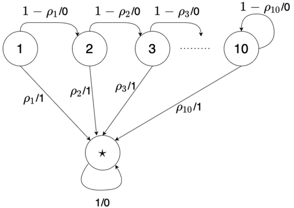 (a) In state , the task is finished with probability or transitions to state with probability . For , the transition from state to state provides 1 as the immediate reward. Otherwise, the agent always receives 0 reward.
|
 (b) Average cumulative regret over 240 simulations.
|
The average regret of the two algorithms is displayed in Figure 5(b). As before, MB-PSRL outperforms MB-UCBVI. Note that we also studied the time to run one simulation for 3000 episodes. This time is around 1 min for MB-PSRL and MB-UCBVI.
0.E.3 Scenario 3: Bayesian Regret and Sensitivity to the Prior
In this section, we study how robust the two implementations of PSRL are, namely MB-PSRL and vanilla PSRL (to simplify, we will just call the later PSRL), to a choice of prior distributions. As explained in Appendix 0.D.2, the natural conjugate prior for Bernoulli reward is the Beta distribution. In this section, we simulate MB-PSRL and PSRL in which the rewards are Bernoulli but the conjugate prior used for the rewards are Gaussian-Gamma which is incorrect for Bernoulli random reward. In other words, MB-PSRL and PSRL have Gaussian-Gamma prior belief while the real rewards are Bernoulli random variables.
To conduct our experiments, we use a Markovian bandit problem with three -state random walk chains represented in Table 1. We draw 16 models by generating 16 pairs of from , 16 pairs of from Dirichlet(3,(1,1,1)) and 16 values of from Dirichlet(2, (1,1)) for each chain. Each model is an unknown MDP that will be learned by MB-PSRL or PSRL. For each of these models, we simulate MB-PSRL and PSRL 5 times with correct priors and 5 times with incorrect priors. The result can be found in Figure 6 which suggests that MB-PSRL performs better when the prior is correct and is relatively robust to the choice of priors in term of Bayesian regret. This figure also shows that PSRL seems more sensitive to the choice of prior distribution. Also note that for both MB-PSRL and PSRL, some trajectories deviate a lot from the mean, under correct priors but even more so with incorrect priors. This illustrates the general fact that learning can go wrong, but with a small probability.
|
MB-PSRL |
 |
 |
 |
|---|---|---|---|
|
PSRL |


Appendix 0.F Experimental environment
The code of all experiments is given in a separated zip file that contains all necessary material to reproduce the simulations and the figures.
Our experiments were run on HPC platform with 1 node of 16 cores of Xeon E5. The experiments were made using Python 3 and Nix and submitted as supplementary material and will be made publicly available with the full release of the paper. The package requirement are detailed in README.md. Using only 1 core of Xeon E5, the Table 2 gives some orders of duration taken by each experiment (with discount factor , and 3000 episodes per simulation). We would like to draw two remarks. First, the duration reported in Figure 1(b) is the time for policy computation (algorithm’s parameters update and policy computation). The duration reported in Table 2 include this plus the computation time for oracle (because we track the regret), the state transition time along the trajectories of oracle and of each algorithm, resetting time… This explains why the duration reported in Table 2 cannot be compared to the duration reported in Figure 1(b). Second, the duration shown in Table 2 are meant to be a rough estimation of the computation time (we only ran the simulation once and the average duration might fluctuate).
| Experiment | MB-PSRL | PSRL | MB-UCRL2 | MB-UCBVI | Total |
| Scenario 1 | 40 min | - | 3days | 50 min | 3days |
| Scenario 2 | 200 min | - | - | 200 min | 400 min |
| Scenario 3 | 90 min | 260 min | - | - | 350 min |