Optimal control of a 2D diffusion-advection process with a team of mobile actuators under jointly optimal guidancefootnoteinfo
Abstract
This paper describes an optimization framework to control a distributed parameter system (DPS) using a team of mobile actuators. The framework simultaneously seeks optimal control of the DPS and optimal guidance of the mobile actuators such that a cost function associated with both the DPS and the mobile actuators is minimized subject to the dynamics of each. The cost incurred from controlling the DPS is linear-quadratic, which is transformed into an equivalent form as a quadratic term associated with an operator-valued Riccati equation. This equivalent form reduces the problem to seeking for guidance only because the optimal control can be recovered once the optimal guidance is obtained. We establish conditions for the existence of a solution to the proposed problem. Since computing an optimal solution requires approximation, we also establish the conditions for convergence to the exact optimal solution of the approximate optimal solution. That is, when evaluating these two solutions by the original cost function, the difference becomes arbitrarily small as the approximation gets finer. Two numerical examples demonstrate the performance of the optimal control and guidance obtained from the proposed approach.
keywords
Infinite-dimensional systems; Multi-agent systems; Modeling for control optimization; Guidance navigation and control.footnoteinfo]This paper was not presented at any IFAC meeting. Corresponding author Sheng Cheng (Tel. +1 301 335 2995).
,
1 Introduction
Recent development of mobile robots (unmanned aerial vehicles, terrestrial robots, and underwater vehicles) has greatly extended the type of distributed parameter system (DPS) over which mobile actuation and sensing can be deployed. Such a system is often modeled by a partial differential equation (PDE), which varies in both time and space. Exemplary applications of mobile control and estimation of a DPS can be found in thermal manufacturing [13], monitoring and neutralizing groundwater contamination [12], and wildfire monitoring [19].
We propose an optimization framework that simultaneously solves for the guidance of a team of mobile actuators and the control of a DPS. We consider a 2D diffusion-advection process as the DPS for its capability of modeling a variety of processes governed by continuum mechanics and the convenience of the state-space representation. The framework minimizes an integrated cost function, evaluating both the control of the DPS and the guidance of the actuators, subject to the dynamics of the DPS and the mobile actuators. The problem addresses the mobile actuator and the DPS as a unified system, instead of solely controlling the DPS. Furthermore, the additional degree of freedom endowed by mobility yields improved control performance in comparison to using stationary actuators.
The study of the control of a PDE-modeled DPS dates back to the 1960s (see the survey [29]). For fundamental results, see the textbooks [7, 28, 1]. Although it is possible to categorize prior work by whether the input operator is bounded, our literature review is categorized by the location of the actuation. When actuation acts on the boundary of the spatial domain, it is called boundary control. The main complexity in boundary control is that the input operator, which associates with the PDE’s boundary condition, is unbounded. This is addressed in the tutorial [15]. Recent developments on the design of boundary control uses the backstepping method [33], where a Volterra transformation determines a stabilizing control by transforming the system into a stable target system. When actuation acts in the interior of the spatial domain, it is called distributed control. For distributed control, the DPS is actuated by in-domain actuators that are either stationary or mobile.
The problem of determining the location of stationary actuators is called the actuator placement problem. Actuator placement has been studied for optimality in the sense of linear-quadratic (LQ) [24], H2 [25], and H∞ [17]. The author of [24] studies the actuator placement problem with the LQ performance criterion. The actuators’ locations are chosen to minimize the operator norm or trace norm of the Riccati operator solved from an algebraic Riccati equation associated with an infinite-dimensional system. If the input operator is compact and continuous with respect to actuator location in the operator norm, then a solution exists for the problem minimizing the operator norm of the Riccati operator [24, Theorem 2.6], under stabilizability and detectability assumptions. When computing the optimal actuator locations, if the approximated Riccati operator converges to the original Riccati operator at each actuator location, then the approximate optimal actuator locations converge to the exact optimal locations [24, Theorem 3.5]. For the above results to hold when minimizing the trace-norm of the Riccati operator, the input and output spaces have to be finite-dimensional [24, Theorems 2.10 and 3.9] in addition to the assumptions stated above.
The authors of [25] design optimal actuator placement by minimizing the H2-control performance criterion, which minimizes the L2-norm of the linear output of a linear system, subject state disturbances. Roughly speaking, H2-control performance reduces the response to the disturbances while setting a zero initial condition, whereas the LQ performance reduces the response to the initial condition in a disturbance-free setting. For disturbances with known or unknown spatial distribution, the trace of the Riccati solution (scaled by the disturbance’s spatial distribution) or operator norm of the Riccati solution are minimized, respectively, where the existence of a solution and convergence to the exact optimal solution of the approximate optimal solution are guaranteed. In [17], the H∞-performance criterion is minimized for actuator placement. Specifically, the actuators are placed in the locations that yield infimum of the attenuation bound (upper bound of the infinity norm of the closed-loop disturbance-to-output transfer function). The conditions for the existence of a solution and convergence to the exact optimal placement of the approximate optimal placement are provided.
Geometric approaches have also been proposed for actuator placement. For example, a modified centroidal Voronoi tessellation (mCVT) yields locations of actuators and sensors that yields least-squares approximate control and estimation kernels for a parabolic PDE [10]. The input operator is designed by maximizing the H2-norm of the input-to-state transfer function, whereas the kernel of the state feedback is obtained using the Riccati solution. Next, mCVT determines the partition such that the actuator and sensor locations achieve optimal performance (in the sense of least-squares) to the input operator and state feedback kernel, respectively. A comparison of various performance criteria for actuator placement has been conducted for controlling a simply supported beam [26] and a diffusion process [27]. It has been analyzed that maximizing the minimum eigenvalue of the controllability gramian is not a useful criterion. Because the lower bound of the eigenvalue is zero, the minimum eigenvalue approaches zero as the dimension of approximation increases [26, 27].
The guidance of mobile actuators is designed to improve the control performance in comparison to stationary actuators. Various performance criteria have been proposed for guidance. In [13], a mobile heat source is steered to maintain a spatially uniform temperature distribution in 1D using the optimal control method. The formulation uses a finite-dimensional approximation for modeling the process and evaluating performance. Additionally, the admissible locations of the heat source are chosen within a discrete set that yields approximate controllability requirements. Algorithms are provided to solve the proposed problem with considerations on real-time implementation and hardware constraints. Experimental results demonstrate the performance of the proposed scheme. The authors of [14] propose an optimization framework that steers mobile actuators to control a reaction-diffusion process. A specific cost function, consisting of norms of control input and measurement of the DPS and the steering force, is minimized subject to dynamics of the actuator’s motion and the PDE, and bounds on the control input and state of the DPS. The implementation of the framework is emphasized by discrete mechanics and model predictive control which yield computationally tractable solutions, in addition to an approximation of the PDE and a discrete set of admissible actuator locations.
The problem of ultraviolet curing using a mobile radiant actuator is investigated in [38], where the curing process is modeled by a 1D nonlinear PDE. Both the radiant power and scanning velocity of the actuator are computed for reaching a target curing state. A dual extended Kalman filter is applied to estimate the state and parameters of the curing process for feedback control, based on the phases of curing. In [11], a navigation problem is studied in which a mobile agent moves through a diffusion process represented by a hazardous field with given initial and terminal positions. Such a formulation may be applied to emergency evacuation guidance from an indoor environment with carbon monoxide. Both problems with minimum time and minimum accumulated effects of hazards are formulated, and closed-form solutions are derived using the Hamiltonian. A Lyapunov-based guidance strategy for collocated sensors and actuators to estimate and control a diffusion process is proposed in [8]. The decentralized guidance of the actuators for controlling a diffusion process to a zero state is derived by constructing suitable Lyapunov functions. The same methodology is applied to construct a distributed consensus filter via the network among agents to improve state estimation. A follow-up work [9] incorporates nonlinear vehicle dynamics in addition.
The problem formulation in this paper includes a cost function that simultaneously evaluates controlling the PDE-modeled DPS, referred to as the PDE cost, and steering the mobile actuators, referred to as the mobility cost. The PDE cost is a quadratic cost of the PDE state and control, whose optimal value can be obtained by solving an operator-valued differential Riccati equation. Our results are based on the related work [3], which establishes Bochner integrable solutions of finite-horizon Riccati integral equations (with values in Schatten p-classes) associated with infinite-dimensional systems. The existence conditions for the solution of exact and approximate Riccati integral equations are established in [3]. The significance of the Bochner integrable solution is that it allows the implementation of simple numerical quadratures for computing the approximated solution of Riccati integral equations. In [3], the Riccati solution is applied in a sensor placement problem, which computes optimal sensor locations that minimize the trace of the covariance operator of the Kalman filter of a diffusion-advection process. The same cost has been used in an optimization framework for mobile sensor’s motion planning in [2]. The existence of a solution of the optimization problem is established under the assumption that the integral kernel of the output operator is continuous with respect to the location of the sensor [2, Definition 4.5]. This assumption permits the construction of a compact set of operators [2, Lemma 4.6] over which the cost function is continuous, and hence establishes the existence of a solution. The assumption is also made on the input operator in this paper, which allows the derivation of a vital result on the Riccati operator’s continuity with respect to the actuator trajectory (Lemma 3). The continuity property plays a crucial role in establishing the existence of the proposed problem’s solution and the convergence to the exact optimal solution of the approximate optimal solution. The existence of a solution is established in using the fact that a weakly sequentially lower semicontinuous function attains its minimum on a weakly sequentially compact set over a normed linear space. In addition to the assumptions made for the existence of a solution, a stringent (yet with reasonable physical interpretation) requirement is placed on the admissible set to yield compactness, which leads to convergence of the approximate optimal solution. The convergence is in the sense that when evaluating the exact and approximate optimal solutions by the original cost function, the difference becomes arbitrarily small as the dimension of approximation increases.
The contributions of this paper are threefold. First, we propose an optimization framework for controlling a PDE-modeled system using a team of mobile actuators. The framework incorporates both controlling the process and steering the mobile actuators. The former is handled by the linear-quadratic regulator of the PDE. The latter is taken care of by designing generic cost functions that address the constraints and limitations of the vehicles carrying the actuators. Second, existence conditions of a solution of the proposed problem are established. It turns out that the conditions are generally satisfied in engineering problems, which allows the results to be applied to a wide range of applications. Third, conditions are also established under which the optimal solution computed using approximations converges to the exact optimal solution. The convergence is in the sense that the cost function of the exact problem evaluated at these two solutions becomes arbitrarily close as the dimensional of the approximation goes to infinity. The convergence is verified in numerical studies and confirms the appropriateness of the optimal solution of the approximation.
The proposed framework is well-suited for the limited onboard resources of mobile actuators in the following two aspects: (1) it adopts a finite-horizon optimization scheme that characterizes the resource limitation more precisely than the alternative approaches that do not specify a terminal time, such as an infinite-horizon optimization or Lyapunov-based method; and (2) it provides an intermediate step for the optimization problem that characterizes the limited resources as inequality constraints, because the constraints can be used to augment the cost function and turned into the proposed form using the method of Lagrange multipliers. Potential applications of this work include forest firefighting using unmanned aerial vehicles and oil spill removal or harmful algae containment using autonomous skimmer boats. A preliminary version of this paper [4] considered controlling a 1D diffusion process by a team of mobile actuators. The results in this paper extends the controlled process in [4] to a 2D diffusion-advection process and generalizes the mobility cost therein. Furthermore, the proofs of the existence of a solution and convergence of the approximated optimal solution are presented for the first time in this paper. The results for a dual estimation framework can be found in [5].
The paper adopts the following notation. The symbols , , and denote the set of real numbers, nonnegative real numbers, and nonnegative integers, respectively. The boundary of a set is denoted by . The -nary Cartesian power of a set is denoted by . A continuous embedding is denoted by . We use and for the norm defined on a finite- and infinite-dimensional space, respectively, with subscript indicating type. The superscript ∗ denotes an optimal variable or an optimal value, whereas ⋆ denotes the adjoint of a linear operator. The transpose of a matrix is denoted by . An -dimensional identity matrix is denoted by . We denote by and an -dimensional matrix with all entries being and , respectively. The term guidance refers to the steering of the mobile actuators, whereas the term control refers to the control input to the DPS. For an optimization problem (P0) that minimizes cost function over variable subject to constraints, we use to denote the cost function of (P0) evaluated at . Specifically, indicates that the optimal value of (P0) is attained when the cost function is evaluated at .
Section II introduces relevant mathematical background, including representation of a diffusion-advection equation by an infinite-dimensional system, the associated LQ optimal control, and its finite-dimensional approximation. Section III introduces the proposed optimization problem and its equivalent problem. Conditions for the existence of a solution are stated. Section IV details the computation of an optimal solution using finite-dimensional approximations. Conditions for the convergence to the exact optimal solution of the approximate optimal solution are stated. A gradient-based method is applied to find an optimal solution. Section V provides two numerical examples to illustrate optimal guidance and control solved by the proposed method. Section VI summarizes the paper and discusses ongoing work.
2 Background
This paper is motivated by the problem of controlling the following diffusion-advection process on a two-dimensional spatial domain with a team of mobile actuators:
| (1) | ||||
| (2) | ||||
| (3) |
where is the state at time , is the velocity field for advection, and is the control implemented by actuator , with the actuation characterized spatially by . The state lives in the state space . A representative model of the actuation dispensed by each actuator is Gaussian-shaped and centered at the actuator ’s location with a bounded support such that
| (4) |
where the parameter determines the spatial influence of the actuation, which is concentrated mostly at the location of the actuator and disperses to the surrounding with an exponential decay.
2.1 Dynamics of the mobile actuators
Assume the mobile actuators have linear dynamics, so that the dynamics of actuator are
| (5) |
where and are the state and guidance at , respectively. Assume that system (5) is controllable. The first two elements of are the horizontal and vertical position, and , of the actuator in the 2D domain. One special case would be a single integrator, where is the position, is the velocity commands, , and .
For conciseness, we concatenate the states and guidance of all actuators, respectively, and use one dynamical equation to characterize the dynamics of all agents:
| (6) |
where matrices and are assembled from and for , respectively and are consistent with the concatenation for and . With a slight abuse of notation, we use for the dimension of and for the dimension of . Define the admissible set of guidance such that for . Let be a matrix such that is a vector of locations of the actuators.
2.2 Abstract linear system and linear-quadratic regulation
To describe the dynamics of PDE (1)–(3), consider the following abstract linear system:
| (7) |
where is the state within state space and is the control within the control space for . In the case of diffusion-advection process (1), for ,
| (8) |
where the operator has domain . The input operator is a function of the actuator locations such that , where for all and . A special case is the time-invariant input operator in (4). Since the actuator state is a function of time , we sometimes use for brevity.
The operator is an infinitesimal generator of a strongly continuous semigroup on . Subsequently, the dynamical system (7) has a unique mild solution for any and any such that .
Similar to a finite-dimensional linear system, a linear-quadratic regulator (LQR) problem can be formulated with respect to (7), which looks for a control that minimizes the following quadratic cost:
| (9) |
where and are self-adjoint and nonnegative, which evaluates the running cost and terminal cost of the PDE state. The coefficient is an -dimensional symmetric and positive definite matrix that evaluates the control effort. We refers to as the PDE cost.
Analogous to the finite-dimensional LQR, an optimal control that minimizes the quadratic cost (9) is
| (10) |
where is an operator that associates with the following backward differential operator-valued Riccati equation:
| (11) |
with terminal condition , where is short for . Before we proceed to state the conditions for the existence of a unique solution of (11), we introduce the -class as follows.
Denote the trace of a nonnegative operator by , where for any orthonormal basis of (the trace is independent of the choice of basis functions). For , let denote the set of all bounded operators such that [3]. If , then the -norm of is defined as . The class and are known as the space of trace operators and the space of Hilbert-Schmidt operators, respectively. Note that a continuous embedding holds if . In other words, if , then and .
The existence of a mild solution of (11) is established via Lemma 1. We omit the proof of this lemma because it is a direct consequence of [3, Theorem 3.6].
Consider the following assumptions with :
- (A1)
and is nonnegative.
- (A2)
and is nonnegative for all .
- (A3)
and is nonnegative for .
Lemma 1.
Let be a separable Hilbert space and let be a strongly continuous semigroup on . Suppose assumptions (A1)–(A3) hold. Then, the equation
| (12) |
provides a unique mild solution to (11) in the space . The solution also belongs to and is pointwise self-adjoint and nonnegative. Furthermore, if and , then is a weak solution to (11).
The equality introduced next in Lemma 2 allows for turning the optimal quadratic PDE cost into a quadratic term associated with the initial condition of the PDE and the Riccati operator. We state it without proof because it can be established by integrating from to ; the differentiability of is proven in [7, Theorem 6.1.9].
Lemma 2.
The following assumption is vital to the main results in this paper.
- (A4)
The input operator is continuous with respect to location [2, Definition 4.5], that is, there exists a continuous function such that and for all , all , and all .
The actuators’ locations determine where the input is actuated and, furthermore, how evolves through (12). Since the input operator is a mapping of the actuators’ locations at time , the composite input operator is a mapping of the actuator state in and so is by (12), although the actuator state is not explicitly reflected in the notation of or . Hence, we can define the optimal PDE cost as a mapping of the actuator state. Let such that . Assumption (A4) plays an important role in yielding the continuity of the mapping stated below in Lemma 3, whose proof is in the supplementary material.
Lemma 3.
Suppose . Let assumptions (A1)–(A3) hold with and be defined as in (12). If assumption (A4) holds, then the mapping such that is continuous.
Approximations to (7) and (12) permit numerical computation. Consider a finite-dimensional subspace with dimension . The inner product and norm of are inherited from that of . Let denote the orthogonal projection of onto . Let and denote the finite-dimensional approximation of and , respectively. A finite-dimensional approximation of (7) is
| (13) | ||||
| (14) |
where and are approximations of and , respectively. Since the actuator state is a function of time , we sometimes use for brevity. Correspondingly, the finite-dimensional approximation of (12) is
| (15) |
where , , and is short for .
The optimal control that minimizes the approximated PDE cost
| (16) |
is analogous to (10):
| (17) |
where is a solution of (15).
The following assumptions are associated with the approximations:
- (A5)
Both and sequence are elements of . Both and are nonnegative for all and as .
- (A6)
Both and sequence are elements of . Both and are nonnegative for all and all and satisfy for all as .
- (A7)
Both and sequence are elements of . Both and are nonnegative for all and all and satisfy
(18) as ( denotes the operator norm).
Note that the assumptions (A1), (A2), and (A3) are contained in (A5), (A6), and (A7), respectively.
The next theorem states the convergence of an approximate solution of the Riccati equation, which is reproduced from [3, Theorem 3.5] and hence stated without a proof.
Theorem 4.
Suppose is a strongly continuous semigroup of linear operators over a Hilbert space and that is a sequence of uniformly continuous semigroup over the same Hilbert space that satisfy, for each
| (19) |
as , uniformly in . Suppose assumptions (A5)–(A7) hold. If is a solution of (12) and is the sequence of solution of (15), then
| (20) |
as .
The following assumption and lemma are analogous to (A4) and Lemma 3, respectively:
- (A8)
The approximated input operator is continuous with respect to location , that is, there exists a continuous function such that and for all , all , and all .
Similar to the mapping in Lemma 3, the optimal approximated PDE cost can be characterized as a mapping of the actuator state through (15), where the continuity is established in Lemma 5, whose proof is in the supplementary material.
Lemma 5.
Suppose . Let assumptions (A5)–(A7) hold and be defined as in (15). If assumption (A8) holds, then the mapping such that is continuous.
3 Problem formulation
This paper seeks to derive the guidance and control input of each actuator such that the state of the abstract linear system (7) can be driven to zero. Specifically, consider the following problem:
| (P) | ||||||
where is the cost associated with the motion of the actuators, named the mobility cost, such that the mappings and evaluate the running state cost and running guidance cost, respectively, and the mapping evaluates the terminal state cost.
The running state cost may characterize restrictions to actuator state. For example, a Gaussian-type function with its peak in the center of the spatial domain, i.e.,
| (21) |
where and , can model a hazardous field that may shorten the life span of an actuator. The integral of this function in the interval evaluates the accumulated exposure of the mobile actuator along its trajectory, which may need to be contained as small as possible (see [11]). Another example is the artificial potential field [16], cast as a soft constraint, that penalizes the trajectory when it passes an inaccessible region such as an obstacle. The running guidance cost may be the absolute value or a quadratic function of the guidance, which characterizes the total amount (of fuel) or energy for steering, respectively. And the terminal state cost may characterize restrictions of the terminal state of the mobile actuators. For example, if an application specifies terminal positions, then may be a quadratic function that penalizes the deviation of the actual terminal positions.
The formulation in (P) provides an intermediate step for minimizing the PDE cost subject to mobility constraints, in addition to the dynamics constraints. The mobility constraints are characterized by inequalities of and the integrals of and , because these constraints can be used to augment the cost function and turned into the form of (P) using the method of Lagrange multipliers.
An equivalent problem of (P) can be derived using Lemma 2. For an arbitrary admissible guidance , the actuator trajectory is determined following the dynamics (6), which also determines the input operator . By Lemma 2, the control that minimizes the cost function of (P)—specifically, the PDE cost —is given by (10), and the minimum PDE cost is , where is the mild solution of (12) with actuator trajectory steered by guidance . Hence, we derive the following problem equivalent to (P):
| (P1) | ||||||
where is defined in (12) with .
To prove the existence of a solution to (P1), we make the following assumptions on the admissible set of guidance and the functions composing the mobility cost:
- (A9)
The set of admissible guidance is closed and convex.
- (A10)
The mappings , , and are continuous. For every , the function is convex.
- (A11)
There exists a constant with for all .
Assumptions (A9)–(A11) are generally satisfied in applications with vehicles carrying the actuators. Assumption (A9) is a physically reasonable characterization of the steering of a vehicle, where the admissible steering is generally a continuum with attainable limits within its range. Assumption (A10) places a general continuity requirement on the cost functions and a convexity requirement on the steering cost function. Assumption (A11) requires the function to be bounded below by a quadratic function of the guidance for all , which is generally satisfied, e.g., with itself being a quadratic function of . These assumptions are applied in Theorem 6 below regarding the existence of a solution of (P1), whose proof is in Appendix A. Subsequently, the solution to (P1) can be used to reconstruct the solutions to (P), which is stated in Theorem 7 with its proof in Appendix B.
Theorem 6.
Theorem 7.
The equivalent problem (P1) allows us to search for an optimal guidance such that the mobility cost plus the optimal PDE cost is minimized. The control is no longer an optimization variable, because it is determined by the LQR of the abstract linear system for arbitrary trajectories of the mobile actuators.
4 Computation of optimal control and guidance
Approximation of the infinite-dimensional terms in problem (P) is necessary when computing the optimal control and guidance. Hence, we replace the PDE cost and dynamics of (P) by (16) and (13), respectively, and obtain the following approximate problem (AP):
| (AP) | ||||||
Similar to (P), problem (AP) can be turned into an equivalent form using LQR results for a finite-dimensional system:
| (AP1) | ||||||
where is defined in (15) with . Analogous to Theorems 6 and 7, the existence of a solution of (AP1) and how to use its solution to reconstruct a solution for (AP) are stated in Theorem 8 below, whose proof is presented in Appendix C.
Theorem 8.
An extension to Theorem 8 is that an optimal feedback control can be obtained from (17) whenever the optimal guidance is solved from (AP) or (AP1). Basically, when the trajectory is determined via the optimal guidance, a feedback control can be implemented.
To establish convergence to the solution of (P1) of (AP1)’s solution, we need to restrict the set of admissible guidance to a smaller set as introduced below in assumption (A12).
- (A12)
There exist and such that the set of admissible guidance is is uniformly bounded by and .
There are two perspectives to interpreting the assumption (A12). Mathematically, (A12) requires the admissible guidance to be a continuous function that is uniformly bounded and uniformly equicontinuous. These two properties yield the sequential compactness of the set by the Arzelà-Ascoli Theorem [30]. Practically, (A12) requires the input signal to be continuous and have bounds and on the magnitude and the rate of change, respectively. This requirement is reasonable and checkable because a continuous signal is commonly used for smooth operation, and the bounds on magnitude and changing rate are due to the physical limits of the motion of a platform. For example, in the case of single integrator dynamics where is the velocity command, and refer to the maximum speed and maximum acceleration, respectively. Moreover, since time discretization of the signal is applied when computing the optimal guidance, as long as the bound on the magnitude of the signal is determined, then the changing rate is bounded by for the smallest discrete interval length . Theorem 9 below states the convergence of the approximate optimal solution with its proof in Appendix D.
Theorem 9.
Remark 10.
Two implications of Theorem 9 follow. First, (22) implies that the optimal cost of the approximated problem (AP1) converges to that of the exact problem (P1), which justifies the approximation in (AP). Second, (23) implies that the approximate optimal guidance , when evaluated by the cost function of (P1), yields a cost that is arbitrarily close to the exact optimal cost of (P1). Since is computable and is not, the convergence in (23) qualifies as an appropriate optimal guidance.
The convergence stated in Theorem 9 is established based on several earlier stated results, including
- 1.
the input operator’s continuity with respect to location (assumption (A4)), which leads to the continuity of the PDE cost with respect to actuator trajectory (Lemma 3);
- 2.
- 3.
sequential compactness of the set of admissible guidance (assumption (A12)), which leads to the continuity of the cost function with respect to guidance (Lemma 12).
Notice that these key results, in an analogous manner, are also required in [24] when establishing the convergence to the exact optimal actuator locations of the approximate optimal locations [24, Theorem 3.5], i.e.,
- 1.
- 2.
- 3.
sequential compactness of the set of admissible locations, which is inherited from the setting that the spatial domain is closed and bounded in a finite-dimensional space.
Although the establishment of convergence is similar to the one in [24], the cost function and type of Riccati equation are different: we have the quadratic PDE cost plus generic mobility cost and differential Riccati equation in this paper for control and actuator guidance versus the Riccati operator’s norm as cost function and algebraic Riccati equation in [24] for actuator placement. The similarity comes from the infinite-dimensional nature of PDEs such that approximation is necessary for computation, and convergence in approximation qualifies the approximate optimal solutions.
4.1 Checking assumptions (A4)–(A12)
For the approximated optimal guidance to be a good proxy of the exact optimal guidance, by Theorem 9, assumption (A4)–(A12) have to be checked to ensure the convergence. We summarize methods for checking these assumptions here. (A4): examine the explicit form of ; (A5)–(A7): examine the explicit form of the operators , , and and their approximations; (A8): examine the explicit form of ; (A9)–(A11): examine the explicit form of ; (A12): examining the bounds on the magnitude and changing rate of the admissible guidance.
4.2 Gradient-descent for solving problem (AP)
Define the costates and associated with and , respectively, for and define the Hamiltonian:
| (24) |
By Pontryagin’s minimum principle [22], we can solve a two-point boundary value problem originated from (24) to find a local minimum of (AP). The iterative procedure for solving the two-point boundary value problem can be implemented in a gradient-descent manner [18, 21].
5 Numerical examples
We demonstrate the performance of the optimal guidance and control in two numerical examples. The first example uses the diffusion-advection process with zero Dirichlet boundary condition (1)–(3). The second example uses the same process but with zero Neumann boundary condition.
The examples are motivated by and simplified from practical applications, e.g., removal of harmful algal blooms (HAB). In this case, the distribution of the HAB’s concentration on the water surface can be modeled by a 2D diffusion-advection process. The cases of zero Dirichlet and Neumann boundary conditions correspond to the scenarios where the surface is circumvented by absorbent and nonabsorbent materials, respectively. The control to the process is implemented by the surface vehicles that use physical methods (e.g., emitting ultrasonic waves or hauling algae filters) or chemical methods (by releasing algal treatment) [32], whose impact on the process can be characterized by the input operator (4). The magnitude of the control determines how fast the concentration is reduced at the location of the actuator. The optimal control and guidance minimize the cost such that the HAB concentration is reduced while the vehicles do not exercise too much control nor conduct aggressive maneuvers. And vehicles’ low-level control can track the optimal trajectories despite the model mismatch between the dynamics of the vehicles and those applied in the optimization problem (P).
We apply the following values in the numerical examples: , , , , , , , , , , , , , , , , , , , , and for , where the indicator function if , and if . We use (4) for the input operator of each actuator. The Péclect number of the process is , which implies neither the diffusion or the advection dominates the process.
5.1 Diffusion-advection process with Dirichlet boundary condition
We use the dynamics in (1)–(3) with the Dirichlet boundary condition. We use the Galerkin scheme to approximate the infinite-dimensional variables. The orthonormal set of eigenfunctions of the Laplacian operator (with zero Dirichlet boundary condition) over the spatial domain is . We introduce a single index such that . For brevity, we use to denote the -dimensional space spanned by the basis functions . Recall the orthogonal projection . It follows that and strongly [3]. Let . We choose because it is the smallest dimension such that the resulting optimal cost is within the 1% of the optimal cost evaluated with the maximum dimension in the numerical studies (see Fig. 7).
Assumption (A4) holds for the choice of input operator. With the Galerkin approximation using the orthonormal eigenfunctions of the Laplacian operator with zero Dirichlet boundary condition, it can be shown that assumption (A8) holds for . Assumptions (A5)–(A7) hold with under the Galerkin approximation with aforementioned basis functions [3]. Assumptions (A9)–(A11) and (A12) hold for the choice of functions in the mobility cost and parameters of the set of admissible guidance, respectively.
We use the forward-backward sweeping method [23] to solve the two-point boundary value problem originated from the Hamiltonian (24). The forward propagation of and and backward propagation of and are computed using the Runge-Kutta method. The same method is also applied to propagate the approximate Riccati solution . Spatial integrals are computed using Legendre-Gauss quadrature. To verify the convergence of the approximate optimal cost stated in (22), we compute for . Note that the total number of basis functions is . The result is shown in Fig. 7, where exponential convergence can be observed.


In the simulation, a mobile disturbance , whose trajectory is is added to the right-hand side of the dynamics (1).
Denote the optimal open-loop control and optimal guidance solved using the gradient-descent method in Section 4.2 by and , respectively. The trajectory steered by is denoted by . Recall that an optimal feedback control, denoted by , can be synthesized using (17) based on the optimal trajectory of the actuators.
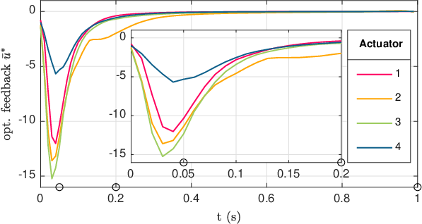
Fig. 1 shows the evolution of the process controlled by the optimal feedback control and the optimal trajectories of the actuators. The actuation concentrates in the first s, which is shown in Fig. 2. Meanwhile, the actuators quickly pass the peak of the initial PDE at the center of the spatial domain and spread evenly in space. Subsequently, the actuators 2–4 cease active steering and dispensing actuation. The flow field causes the actuators to drift until the terminal time.
To demonstrate the performance of the optimal feedback control , we compare it with semi-naive control and naive control defined as local feedback controls: and . The semi-naive actuators follow the optimal trajectory , whereas the naive actuators follow the trajectory , which moves at a constant speed from to . Table 1 compares the cost breakdown of all the control and guidance strategies. The optimal feedback control yields a smaller cost than the optimal open-loop control due to the capability of feedback control in rejecting disturbances. Simulations with a disturbance-free model (not shown) yield identical total cost for optimal open-loop control and optimal feedback control, which justifies the correctness of the synthesis. Fig. 3 compares the norm of the PDE state controlled by pairs of control and guidance listed in Table 1. As can be seen, the PDE is effectively regulated using optimal feedback control. As a comparison, the norm associated with optimal open-loop control grows slowly after s due the influence of the disturbance, although its reduction in the beginning is indistinguishable from that of the optimal feedback control.
| Control (C) and Guidance (G) | Cost | |||||
|---|---|---|---|---|---|---|
| C | G | Total | ||||
| opt. feedback | 13.7% | 3.0% | 16.7% | |||
| opt. open-loop | 17.5% | 3.0% | 20.5% | |||
| semi-naive | 42.5% | 3.0% | 45.5% | |||
| naive | 78.8% | 0.5% | 79.3% | |||
| no control | - | - | 100.0% | 0.0% | 100.0% | |
5.2 Diffusion-advection process with Neumann boundary condition
The results derived in this paper also apply to the operator defined in (8) with a Neumann boundary condition (BC), because a general second-order and uniformly elliptic operator with Neumann BC yields a strongly continuous analytic semigroup on [20]. In this example, we consider the diffusion-advection process (1) with initial condition (3) and zero Neumann BC: , where is the normal to the boundary and . Notice that the basis functions applied for Galerkin approximation in this case are the eigenfunctions of the Laplacian with zero Neumann BC, for . All the parameters, disturbance, and pairs of control and guidance for comparison applied in this example are identical to those in Section 5.1. Exponential convergence in the approximate optimal cost can be observed in Fig. 7.
Fig. 4 shows the evolution of the process and the optimal trajectory of the actuators. Similar to the case of Dirichlet BC, the actuators spread out to cover most of the domain in the initial s, with most of the actuation implemented during the same interval, seen in Fig. 5. However, the actuators span a slightly larger area (Fig. 4) and the maximum amplitude of actuation is bigger (Fig. 5), compared to the case of Dirichlet BC in Fig. 1 and Fig. 2, respectively. The difference is a consequence of the fact that the zero Neumann BC does not contribute to the regulation of the process because it insulates the process from the outside. Contrarily, the zero Dirichlet BC acts as a passive control that can essentially regulate the process to a zero state when there is no inhomoegeneous term in the dynamics (1). This difference can be observed when comparing the norm of the PDE state in Fig. 6 with Fig. 3. The norm of the uncontrolled state reduces slightly in the case of Neumann BC (Fig. 6) compared to the almost linear reduction in the case of Dirichlet BC (Fig. 3). Fig. 6 also shows the difference of norm reduction between the optimal feedback control and optimal open-loop control. Once again, the former yields a smaller terminal norm than the latter due to the feedback’s capability of disturbance rejection. The cost breakdown of the pairs of control and guidance in comparison is shown in Table. 2.


| Control (C) and Guidance (G) | Cost | |||||
|---|---|---|---|---|---|---|
| C | G | Total | ||||
| opt. feedback | 6.4% | 1.6% | 8.0% | |||
| opt. open-loop | 7.1% | 1.6% | 8.7% | |||
| semi-naive | 63.7% | 1.6% | 65.3% | |||
| naive | 65.9% | 0.2% | 66.1% | |||
| no control | - | - | 100.0% | 0.0% | 100.0% | |

6 Conclusion
This paper proposes an optimization framework that steers a team of mobile actuators to control a DPS modeled by a 2D diffusion-advection process. Specifically, jointly optimal control of the DPS and guidance of the mobile actuators are solved such that the sum of a quadratic PDE cost and a generic mobility cost is minimized subject to the dynamics of the DPS and of the mobile actuators. We obtain an equivalent problem using LQR of an abstract linear system, which reduces the problem to search for optimal guidance only. The optimal control can be synthesized once the optimal guidance is obtained. Conditions on the existence of a solution are established based on the equivalent problem. We use the Galerkin approximation scheme to reduce the problem to a finite-dimensional one and apply a gradient-descent method to compute optimal guidance and control numerically. We prove conditions under which the approximate optimal guidance converges to that of the exact optimal guidance in the sense that when evaluating these two solutions by the original cost function, the difference becomes arbitrarily small as the dimension of approximation increases. The convergence justifies the appropriateness of both the approximate problem and its solution. The performance of the proposed optimal control and guidance is illustrated with two numerical examples , where exponential convergence of the approximate optimal cost is observed.
Ongoing and future work includes establishing the convergence rate of the approximate optimal cost and studying problems with other types of PDE cost, such as the operator norm of the Riccati operator [24, 6] to characterize unknown initial conditions and H2- or H∞-performance criteria for different types of perturbation [25, 17]. On the actuator side, decentralized guidance design may be incorporated in future work to enable more autonomy of the team than a centralized implementation. Actuators that travel along the boundary may be considered as well which would result in boundary controller design.
Appendix A Proof of Theorem 6
Theorem 11.
[36, Theorem 6.1.4] Suppose is a normed linear space, is weakly sequentially compact and is weakly sequentially lower semicontinuous on . Then there exists an such that .
Proof of Theorem 6
Without loss of generality, we consider the case of one mobile actuator, i.e., . The case of follows naturally.
We want to apply Theorem 11 to prove that the minimum of the cost function of (P1) is achieved on a subset (defined below) of the admissible set in which the cost of guidance is upper bounded. Consider problem (P1)’s admissible set of guidance functions . Assume there exists such that and let . We wish to prove Condition-1, Condition-2, and Condition-3 stated below:
Condition-1: The set is bounded.
Condition-2: The set is weakly sequentially closed.
Condition-3: The mapping is weakly sequentially lower semicontinuous on .
Condition-1 and Condition-2 imply that is weakly sequentially compact. By Theorem 11, problem (P1) has a solution when Condition-1–Condition-3 hold.
Before proving these three conditions, we define a mapping by for . For and , we have
| (25) |
for and . Hence, , which also shows that is a continuous mapping, i.e., for all .
Proof of Condition-1: Suppose , then
| (26) |
where the second inequality follows from the nonnegativity of , and . Since , the boundedness of follows.
Proof of Condition-2: Suppose and converges weakly to (denoted by ). We want to show . We start with proving that is weakly sequentially closed and, hence, . Subsequently, we show to conclude Condition-2.
To show that the set is weakly sequentially closed, by [35, Theorem 2.11], it suffices to show that is closed and convex. Let and . We want to show , i.e., and for . Since is complete, we can choose a subsequence that converges to pointwise almost everywhere on [37, p. 53]. Since is closed (assumption (A9)), for almost all . Hence, is closed. The convexity of follows from that of (assumption (A9)), i.e., if , then and for and .
What remain to be shown is . Since , by definition, we have . We now show that the sequence contains a uniformly convergent subsequence in . The sequence is uniformly bounded and uniformly equicontinuous for the following reasons: Since , it follows that is uniformly bounded, because which is a bounded set. For , we have
Since and both are uniformly bounded for all , is uniformly equicontinuous. By the Arzelà-Ascoli Theorem [30], there is a uniformly convergent subsequence .
Without loss of generality, we assume and uniformly on , and . We have , by which, to show , it suffices to show , which is to show
| (27) |
where is the solution of (12) associated with actuator state . Since converges to uniformly on , the continuity of implies
| (28) |
Fatou’s lemma [30] implies
| (29) |
and Lemma 3 implies
| (30) |
To prove (27), based on (28)–(30), it suffices to show . By contradiction, assume there is such that
| (31) |
There exists a subsequence such that
and .
We wish to show that is weakly sequentially closed. By [35, Theorem 2.11], it suffices to show that is convex and closed. Since is convex for all , it follows that is convex. Let and converges to as . We can choose a subsequence such that converges to pointwise almost everywhere on [37, p. 53]. Now we have
(1) for all (assumption (A11));
(2) almost everywhere on .
Since is weakly sequentially closed, implies that , which contradicts (31). Hence, is proved, and we conclude Condition-2.
Proof of Condition-3: We now show that the mapping is weakly sequentially lower semicontinuous on . Suppose and . We wish to show , which has been established when we proved in Condition-2 (starting from (27)).
So we conclude that the existence of a solution of problem (P1). ∎
Appendix B Proof of Theorem 7
Proof
By contradiction, assume there are and minimizing (P) and and such that . Denote the optimal control (10) associated with actuator trajectory steered by . It follows that , because violates the optimality of and contradicts the fact that minimizes the quadratic cost (see Lemma 2). Since , where associates with trajectory steered by , it follows that is not an optimal solution of (P1), which contradicts the optimality of for (P1).∎
Appendix C Proof of Theorem 8
Appendix D Proof of Theorem 9
Before we prove Theorem 9, we first establish two intermediate results in Lemma 12, whose proof is in the supplementary material.
Lemma 12.
Consider problem (P1) and its approximation (AP1). If assumptions (A4)–(A7) and (A9)–(A12) hold, then the following two implications hold:
1. For , , where is the dimension of approximation applied in (AP).
2. The mapping is continuous, where . Here, the actuator state follows the dynamics (6) steered by the guidance , and follows (11) with the actuator state .
Proof of Theorem 9
In the notation , the dimension of approximation in (AP1), which is in this case, is indicated by its solution . We append a subscript to indicate the dimension when it is not explicitly reflected by the argument, e.g., .
To proceed with proving (22), in addition to (32), we shall show . Choose a convergent subsequence such that . Since the guidance functions defined in the set are uniformly equicontinuous and uniformly bounded, by the Arzelà-Ascoli Theorem [30], there is a uniformly convergent subsequence of which we use the same index to simplify notation and let the limit of be , i.e.,
| (33) |
Now, , which implies
| (34) |
The first limit on the right-hand side of (34) is zero for the following reason. For all , converges to pointwise as the dimension of approximation (see Lemma 12-1). Furthermore, since the sequence of approximated PDE cost is a monotonically increasing sequence, the sequence is a monotonically increasing sequence for each on the compact set . By Dini’s Theorem [31, Theorem 7.13], uniformly on as . By Moore-Osgood Theorem [31, Theorem 7.11], this uniform convergence and the convergence as (see (33)) imply that , in which the iterated limit equals the double limit [34, p. 140], i.e.,
The second limit on the right-hand side of (34) is zero due to Lemma 12-2. Hence, it follows from (34) that , which implies
| (35) |
Next, we show (23), i.e., as . We start with for all , which implies that
| (36) |
To prove (23), what remains to be shown is . Choose a convergent subsequence such that . Since is uniformly equicontinuous and uniformly bounded, by Arzelà-Ascoli Theorem [30], the sequence has a (uniformly) convergent subsequence which we denote with the same indices to simplify notation. Denote the limit of by such that
| (37) |
Due to the continuity of (see Lemma 12-1), we have
It follows that
| (38) |
Since the sequence of approximated PDE cost is monotonically increasing, the sequence is a monotonically increasing sequence for each on the compact set . Since for all (see Lemma 12-1), by Dini’s Theorem [31, Theorem 7.13], the limit holds uniformly on as . By Moore-Osgood Theorem [31, Theorem 7.11], this uniform convergence and the convergence as (see (37)) imply that
| (39) |
Furthermore, the iterated limit equals the double limit [34, p. 140], i.e.,
| (40) |
Hence, combining (38)–(40), we have , from which and (36) we conclude the desired convergence . ∎
References
- [1] A. Bensoussan, G. Da Prato, M. C. Delfour, and S. K. Mitter. Representation and control of infinite dimensional systems, volume 1. Birkhäuser Boston, 1992.
- [2] J. A. Burns and C. N. Rautenberg. The infinite-dimensional optimal filtering problem with mobile and stationary sensor networks. Numer. Funct. Anal. Optim., 36(2):181–224, 2015.
- [3] J. A. Burns and C. N. Rautenberg. Solutions and approximations to the riccati integral equation with values in a space of compact operators. SIAM J. Control Optim., 53(5):2846–2877, 2015.
- [4] S. Cheng and D. A. Paley. Optimal control of a 1D diffusion process with a team of mobile actuators under jointly optimal guidance. In Proc. 2020 American Control Conf., pages 3449–3454, 2020.
- [5] S. Cheng and D. A. Paley. Optimal guidance and estimation of a 2D diffusion-advection process by a team of mobile sensors. Submitted, 2021.
- [6] S. Cheng and D. A. Paley. Optimal guidance of a team of mobile actuators for controlling a 1D diffusion process with unknown initial conditions. In Proc. American Control Conf., pages 1493–1498, 2021.
- [7] R. F. Curtain and H. Zwart. An introduction to infinite-dimensional linear systems theory, volume 21. Springer Science & Business Media, 2012.
- [8] M. A. Demetriou. Guidance of mobile actuator-plus-sensor networks for improved control and estimation of distributed parameter systems. IEEE Trans. Automat. Control, 55(7):1570–1584, 2010.
- [9] M. A. Demetriou. Adaptive control of 2-D PDEs using mobile collocated actuator/sensor pairs with augmented vehicle dynamics. IEEE Trans. Automat. Control, 57(12):2979–2993, 2012.
- [10] M. A. Demetriou. Using modified Centroidal Voronoi Tessellations in kernel partitioning for optimal actuator and sensor selection of parabolic PDEs with static output feedback. In Proc. 56th IEEE Conf. Decision and Control, pages 3119–3124, 2017.
- [11] M. A. Demetriou and E. Bakolas. Navigating over 3D environments while minimizing cumulative exposure to hazardous fields. Automatica, 115:108859, 2020.
- [12] M. A. Demetriou and I. I. Hussein. Estimation of spatially distributed processes using mobile spatially distributed sensor network. SIAM J. Control Optim., 48(1):266–291, 2009.
- [13] M. A. Demetriou, A. Paskaleva, O. Vayena, and H. Doumanidis. Scanning actuator guidance scheme in a 1-D thermal manufacturing process. IEEE Trans. Control Systems Technology, 11(5):757–764, 2003.
- [14] S. Dubljevic, M. Kobilarov, and J. Ng. Discrete mechanics optimal control (DMOC) and model predictive control (MPC) synthesis for reaction-diffusion process system with moving actuator. In Proc. 2010 American Control Conf., pages 5694–5701, 2010.
- [15] Z. Emirsjlow and S. Townley. From PDEs with boundary control to the abstract state equation with an unbounded input operator: a tutorial. Eur. J. Control, 6(1):27–49, 2000.
- [16] M. Hoy, A. S. Matveev, and A. V. Savkin. Algorithms for collision-free navigation of mobile robots in complex cluttered environments: a survey. Robotica, 33(3):463–497, 2015.
- [17] D. Kasinathan and K. Morris. H∞-optimal actuator location. IEEE Trans. Automat. Control, 58(10):2522–2535, 2013.
- [18] D. E. Kirk. Optimal control theory: an introduction. Courier Corporation, 2012.
- [19] M. Kumar, K. Cohen, and B. HomChaudhuri. Cooperative control of multiple uninhabited aerial vehicles for monitoring and fighting wildfires. J. Aerospace Computing, Information, and Communication, 8(1):1–16, 2011.
- [20] I. Lasiecka and R. Triggiani. Control theory for partial differential equations: continuous and approximation theories, volume 1. Cambridge University Press Cambridge, 2000.
- [21] F. L. Lewis, D. Vrabie, and V. L. Syrmos. Optimal control. John Wiley & Sons, 2012.
- [22] D. Liberzon. Calculus of variations and optimal control theory: a concise introduction. Princeton University Press, 2011.
- [23] M. McAsey, L. Mou, and W. Han. Convergence of the forward-backward sweep method in optimal control. Comput. Optim. Appl., 53(1):207–226, 2012.
- [24] K. Morris. Linear-quadratic optimal actuator location. IEEE Trans. Automat. Control, 56(1):113–124, 2010.
- [25] K. Morris, M. A. Demetriou, and S. D. Yang. Using H2-control performance metrics for the optimal actuator location of distributed parameter systems. IEEE Trans. Automat. Control, 60(2):450–462, 2015.
- [26] K. Morris and S. Yang. Comparison of actuator placement criteria for control of structures. J. Sound and Vibration, 353:1–18, 2015.
- [27] K. Morris and S. Yang. A study of optimal actuator placement for control of diffusion. In Proc. 2016 American Control Conf., pages 2566–2571, 2016.
- [28] S. Omatu and J. H. Seinfeld. Distributed parameter systems: theory and applications. Clarendon Press, 1989.
- [29] A. C. Robinson. A survey of optimal control of distributed-parameter systems. Automatica, 7(3):371–388, 1971.
- [30] H. Royden and P. Fitzpatrick. Real analysis (4th edition). New Jersey: Prentice-Hall Inc, 2010.
- [31] W. Rudin. Principles of mathematical analysis, volume 3.
- [32] A. Schroeder. Mitigating harmful algal blooms using a robot swarm. PhD thesis, University of Toledo, 2018.
- [33] A. Smyshlyaev and M. Krstic. Adaptive control of parabolic PDEs. Princeton University Press, 2010.
- [34] A. E. Taylor. General theory of functions and integration. Courier Corporation, 1985.
- [35] F. Tröltzsch. Optimal control of partial differential equations: theory, methods, and applications, volume 112. American Mathematical Society, 2010.
- [36] J. Werner. Optimization theory and applications. Springer-Verlag, 2013.
- [37] K. Yosida. Functional analysis, volume 123. springer, 1988.
- [38] F. Zeng and B. Ayalew. Estimation and coordinated control for distributed parameter processes with a moving radiant actuator. J. Process Control, 20(6):743–753, 2010.