跳到论文正文
W Papers独立论文阅读器 arXiv:2106.08051 论文正文 计算阅读时间 · 0%
引用这篇论文根据当前论文元数据生成,正式投稿前建议核对。


License: CC BY-NC-ND 4.0
arXiv:2106.08051v2 [math.PR] 25 Jan 2022

Convergence of the KPZ line ensemble

Xuan Wu Address: Department of Mathematics, University of Chicago, Chicago IL, 60637 Email address: xuanw@uchicago.edu
Abstract.

In this paper we study the KPZ line ensembles under the KPZ scaling. Based on their Gibbs property, we derive quantitative local fluctuation estimates for the scaled KPZ line ensembles. This allows us to show that the family of scaled KPZ line ensembles is tight. Together with the recent progresses in [QS20], [Vir] and [DM], the tightness result yields the conjectural convergence of the scaled KPZ line ensembles to the Airy line ensemble.

1. Introduction

1.1. Kardar-Parisi-Zhang equation

The main object of study in this paper, the KPZ line ensemble, can be viewed as a multi-layer extension to the well-known Kardar-Parisi-Zhang (KPZ) equation. The KPZ equation was introduced in 1986 by Kardar, Parisi and Zhang [KPZ] as a model for random interface growth. In one-spatial dimension (sometimes also called (1+1)-dimension to emphasize that time is one dimension too), it describes the evolution of a function ℋ⁡(t,x)\mathcal{H}(t,x) recording the height of an interface at time t>0t>0 above position x∈ℝx\in\mathbb{R}. The KPZ equation is written formally as a stochastic partial differential equation (sPDE),

(1.1) ∂tℋ=12​∂x2ℋ+12​(∂xℋ)2+𝒲˙,\partial_{t}\mathcal{H}=\frac{1}{2}\partial_{x}^{2}\mathcal{H}+\frac{1}{2}(\partial_{x}\mathcal{H})^{2}+\mathscr{\dot{W}},

where 𝒲˙\mathscr{\dot{W}} is a space-time white noise (for mathematical background or literature review, see [Cor, QS15] for instance).

The KPZ equation (1.1) is associated with a famous universality class, the KPZ universality class, which bears the same name. The KPZ equation is a canonical member of the associated KPZ universality class and a model belongs to the KPZ universality class if it bears the same long-time, large-scale behavior as the KPZ equation. The KPZ universality class hosts a large class of models, which covers a wide range of mathematical and physical systems of distinct origins, including interacting particle systems, random matrices, traffic models, directed polymers in random media and non-linear stochastic PDEs.

All models in the KPZ universality class can be transformed to a kinetically growing interface reflecting the competition between growth in a direction normal to the surface, a surface tension smoothing force, and a stochastic term which tends to roughen the interface. These features may be illustrated by the Laplacian 12​∂x2ℋ\frac{1}{2}\partial_{x}^{2}\mathcal{H}, non-linear term 12​(∂xℋ)2\frac{1}{2}(\partial_{x}\mathcal{H})^{2} and white noise 𝒲˙\mathscr{\dot{W}} in the KPZ equation (1.1). Numerical simulations along with some theoretical results have confirmed that in the long time tt scaling limit, fluctuations in the height of such evolving interfaces scale like t1/3t^{1/3} and display non-trivial spatial correlations in the scale t2/3t^{2/3} (known as the 3:2:13:2:1 KPZ scaling).

The KPZ equation is related to the stochastic heat equation (SHE) with multiplicative noise through the Hopf–Cole transformation. Denote 𝒵⁡(t,x)\mathcal{Z}(t,x) as the solution to the following SHE,

(1.2) ∂t𝒵=12​∂x2𝒵+𝒵​𝒲˙.\partial_{t}\mathcal{Z}=\frac{1}{2}\partial_{x}^{2}\mathcal{Z}+\mathcal{Z}\mathscr{\dot{W}}.

The Hopf-Cole solution to the KPZ equation (1.1) is defined through taking

ℋ⁡(t,x)=log⁡𝒵⁡(t,x).\mathcal{H}(t,x)=\log\mathcal{Z}(t,x).

It was first proved in [Mue] that 𝒵⁡(t,x)\mathcal{Z}(t,x) is almost surely strictly positive (with positive initial conditions), which justifies the validity of the transform. The fundamental solution 𝒵n​w​(t,x)\mathcal{Z}^{nw}(t,x) to SHE (1.2) is of great importance. It solves (1.2) with a delta mass initial value at origin, i.e. 𝒵⁡(0,x)=δx=0\mathcal{Z}(0,x)=\delta_{x=0}. Meanwhile ℋn​w​(t,x)=log⁡𝒵n​w​(t,x)\mathcal{H}^{nw}(t,x)=\log\mathcal{Z}^{nw}(t,x) is known as the narrow wedge solution to the KPZ equation. The initial condition of ℋn​w​(0,x)\mathcal{H}^{nw}(0,x) is not well-defined; however ℋn​w​(t,x)\mathcal{H}^{nw}(t,x) is stationary around a parabola −x22​t\frac{-x^{2}}{2t}, which resembles a sharp wedge for small tt, hence known as the narrow wedge initial condition.

Using the Feynman-Kac representation, 𝒵n​w​(t,x)\mathcal{Z}^{nw}(t,x) formally takes the following expression,

(1.3) 𝒵n​w(t,x)=p(t,x)𝔼[:exp:(∫0t𝒲˙(s,Bs)ds)],\mathcal{Z}^{nw}(t,x)=p(t,x)\mathbb{E}\left[:\exp:\left(\int_{0}^{t}\mathscr{\dot{W}}(s,B_{s})ds\right)\right],

where p(t,x)=(2πt)−1/2exp(−x2/2t)p(t,x)=(2\pi t)^{-1/2}\exp(-x^{2}/2t) is the heat kernel, the expectation is taken with respect to a Brownian bridge (Bs,s≤t)(B_{s},s\leq t) which starts at origin at time 00 and arrives at xx at time tt. The :exp::{\rm exp}: is the Wick exponential, see [Jan] for instance. This bridge representation arises because of the δx=0\delta_{x=0} initial condition, and hence the factor p⁡(t,x)p(t,x). This Feynman-Kac representation is mostly formal since the integral of white noise over a Brownian path is not well-defined pathwise or to exponentiate the integral.

We adopt this representation to emphasize on its interpretation as being the partition function of a continuum directed random polymer (CDRP) that is modeled by a continuous path interacting with a space-time white noise. We emphasize that this approach is very useful for a generalization to the multi-layer scenario which involves multiple Brownian bridges, see an illustration in Figure 1. We will make sense of the expression (1.3) through a chaos expansion after we introduce its multi-layer extension below.

Refer to caption Refer to caption
Figure 1. On the left, the CDRP can be formulated in terms of the general directed polymer framework, i.e. a random path interacting with a random environment. More precisely, the underlying path measure is that of a Brownian bridge which starts at 00 at time 00 and ends at xx at time tt; and the random environment is the white noise 𝒲˙\mathscr{\dot{W}}. The multi-layer extension on the right involves non-intersecting Brownian bridges and is defined similarly.

1.2. The KPZ line ensemble and CDRP partition functions

Motivated by recent developments on solvable directed polymer models, [OW] generalizes the above Feynman-Kac representation / continuum polymer partition function 𝒵⁡(t,x)\mathcal{Z}(t,x) to accommodate multiple non-intersecting Brownian bridges. More precisely, they defined a hierarchy of partition functions 𝒵n​(t,x)\mathcal{Z}_{n}(t,x), formally written as

(1.4) 𝒵n(t,x)=p(t,x)n𝔼[:exp:{∑i=1n∫0t𝒲˙(s,Bi(s))ds}],\mathcal{Z}_{n}(t,x)=p(t,x)^{n}\mathbb{E}\left[:{\rm exp}:\,\left\{\sum_{i=1}^{n}\int_{0}^{t}\mathscr{\dot{W}}(s,B_{i}(s))ds\right\}\right],

where the expectation is taken with respect to the law on nn independent Brownian bridges {Bi}i=1n\{B_{i}\}_{i=1}^{n} starting at 00 at time 00 and ending at xx at time tt. Intuitively these path integrals represent energies of non-intersecting paths, and thus the expectation of their exponential represents the partition function for this path (or directed polymer) model. It is worth noting that the first layer, 𝒵1\mathcal{Z}_{1}, is the sames as the fundamental solution 𝒵n​w\mathcal{Z}^{nw} to the SHE (1.2). These partition functions 𝒵n​(t,x)\mathcal{Z}_{n}(t,x) also solve a multi-layer extension of SHE (1.2), see [OW].

For n∈ℕn\in\mathbb{N}, t≥0t\geq 0 and x∈ℝx\in\mathbb{R}, 𝒵n​(t,x)\mathcal{Z}_{n}(t,x) is rigorously defined via the following chaos expansion,

(1.5) 𝒵n(t,x)=p(t,x)n∑k=0∞∫Δk​(t)∫ℝkRk(n)((t1,x1),⋯,(tk,xk))𝒲˙(dt1dx1)⋯𝒲˙(dtkdxk),\mathcal{Z}_{n}(t,x)=p(t,x)^{n}\sum_{k=0}^{\infty}\int_{\Delta_{k}(t)}\int_{\mathbb{R}^{k}}R_{k}^{(n)}\left((t_{1},x_{1}),\cdots,(t_{k},x_{k})\right)\mathscr{\dot{W}}(dt_{1}dx_{1})\cdots\mathscr{\dot{W}}(dt_{k}dx_{k}),

where Δk(t)={0<t1<⋯<tk<t}\Delta_{k}(t)=\{0<t_{1}<\cdots<t_{k}<t\}, and Rk(n)R_{k}^{(n)} is the kk-point correlation function for a collection of nn non-intersecting Brownian bridges each of which starts at 00 at time 00 and ends at xx at time tt. For notational simplicity, set 𝒵0​(t,x)≡1\mathcal{Z}_{0}(t,x)\equiv 1. For details about integration with respect to a white noise, we refer to [Jan].

[LW] show that for any t>0t>0, with probability 1, for all x∈ℝx\in\mathbb{R} and all n∈ℕn\in\mathbb{N}, 𝒵n​(t,x)>0\mathcal{Z}_{n}(t,x)>0. The positivity result permits the following important definition of the KPZ line ensemble ℋnt​(x)\mathcal{H}_{n}^{t}(x), a process given by the logarithm of ratios of partition functions 𝒵n\mathcal{Z}_{n}.

Definition 1.1.

For t>0t>0 fixed, the KPZ line ensemble is a continuous ℕ\mathbb{N}-indexed line ensemble ℋt={ℋnt}n∈ℕ\mathcal{H}^{t}=\{\mathcal{H}^{t}_{n}\}_{n\in\mathbb{N}} on ℝ\mathbb{R} given by

(1.6) ℋnt​(x):=log⁡(𝒵n​(t,x)𝒵n−1​(t,x)),\mathcal{H}^{t}_{n}(x):=\log\left(\frac{\mathcal{Z}_{n}(t,x)}{\mathcal{Z}_{n-1}(t,x)}\right),

with convention 𝒵0≡1\mathcal{Z}_{0}\equiv 1. Note that ℋ1t​(⋅)\mathcal{H}^{t}_{1}(\cdot) equals ℋn​w​(t,⋅)\mathcal{H}^{nw}(t,\cdot), the time tt spatial process of the Hopf-Cole solution to the KPZ equation (1.1) with narrow-wedge initial data. Sometimes we will omit tt and just write the KPZ line ensemble as ℋ\mathcal{H}.

Refer to caption
Figure 2. An overview of KPZt\textrm{KPZ}_{t} line ensemble ℋt\mathcal{H}^{t} for fixed time tt. Curves ℋ1t​(⋅)\mathcal{H}^{t}_{1}(\cdot) through ℋ4t​(⋅)\mathcal{H}^{t}_{4}(\cdot) are sampled. The lowest indexed curve ℋ1t\mathcal{H}^{t}_{1} is distributed according to the time tt solution to KPZ equation with narrow wedge initial data. The dotted first two curves ℋ1t\mathcal{H}^{t}_{1} and ℋ2t\mathcal{H}^{t}_{2} between aa and bb indicate a possible resampling according to two independent Brownian bridges which subject to an exponential penalization for going out of order (Definition 2.4), as a demonstration for the 𝐇\mathbf{H}-Brownian Gibbs property.

The KPZ line ensemble arises as scaling limits of O’Connell-Yor semi-discrete direct polymers [OY] and log-gamma discrete directed polymers [Sep]. For O’Connell-Yor semi-discrete direct polymers, the convergence follows from the subsequential compactness result in [CH16] and finite dimensional convergence in [Nic]. The Gibbs property of ℋ\mathcal{H} was introduced in [CH16], which plays a key role in their investigation. The analogue result about sequential compactness and limiting Gibbs property for log-gamma line ensemble was carried out in [Wu19].

1.3. 𝐇\mathbf{H}-Brownian Gibbs property

In this subsection, we describe the key tool we exploit in this paper, the 𝐇\mathbf{H}-Brownian Gibbs property of the KPZ line ensemble.

An 𝐇\mathbf{H}-Brownian Gibbs property can be viewed as a resampling invariance. Let ℒ={ℒ1,ℒ2,…}\mathcal{L}=\{\mathcal{L}_{1},\mathcal{L}_{2},\dots\} be a line ensemble, i.e., countably many random functions indexed by ℕ\mathbb{N}. We may also view ℒ\mathcal{L} as a random variable taking values in C⁡(ℕ×ℝ,ℝ)C(\mathbb{N}\times\mathbb{R},\mathbb{R}). Then ℒ\mathcal{L} satisfies the 𝐇\mathbf{H}-Brownian Gibbs property if for any integers k1≤k2k_{1}\leq k_{2} and [a,b]⊂ℝ[a,b]\subset\mathbb{R}, the law of ℒ\mathcal{L} is unchanged if one replaces the restriction of ℒ\mathcal{L} on [k1,k2]ℤ×[a,b][k_{1},k_{2}]_{\mathbb{Z}}\times[a,b] by independent Brownian bridges, re-weighted by an interaction factor (determined by H) between adjacently indexed curves. See Definition 2.3 for the precise definition.

There is a large class of stochastic integrable models from random matrix theory, interacting particle systems, last passage percolation and directed polymers that enjoy certain 𝐇\mathbf{H}-Brownian Gibbs properties. Among them, the parabolic Airy line ensemble 𝒜~\tilde{\mathcal{A}} (defined in Definition 1.7 in the next subsection) is the most celebrated one and it satisfies the 𝐇ord\mathbf{H}_{\textup{ord}}-Brownian Gibbs property. See Definition 2.5 for the expression of 𝐇ord\mathbf{H}_{\textup{ord}}. We remark that in the literature, the 𝐇ord\mathbf{H}_{\textup{ord}}-Brownian Gibbs property is referred to as the Brownian Gibbs property.

After the discovery of the 𝐇ord\mathbf{H}_{\textup{ord}}-Brownian Gibbs property of 𝒜~\tilde{\mathcal{A}} in [CH14], this Gibbs property has served as a powerful probability tool in studying the Airy line ensemble and other line ensembles enjoying same Gibbs property. Recently, one of the authors of [CH14], developed a more delicate treatment in [Ham1] to estimate the modulus of continuity for line ensembles with the 𝐇ord\mathbf{H}_{\textup{ord}}-Brownian Gibbs property (e.g. the Airy line ensemble and the line ensemble associated with Brownian last passage percolation). [Ham1] also established L∞−L^{\infty-} bounds on the Radon-Nikodym derivative of the line ensemble curves with respect to Brownian bridges and other refined regularity properties. Furthermore in the subsequent papers [Ham2, Ham3, Ham4], the work in [Ham1] was applied to understanding the geometry of last passage paths in Brownian last passage percolation with more general initial data. Another breakthrough is the construction of the directed landscape [DOV], based on the 𝐇ord\mathbf{H}_{\textup{ord}}-Brownian Gibbs property of the Brownian last passage percolation.

The KPZ line ensemble (defined in Definition 1.1) is an central integrable model in the KPZ universality class. It satisfies the 𝐇\mathbf{H}-Brownian Gibbs property with 𝐇⁡(x)=ex\mathbf{H}(x)=e^{x}. In view of the successful applications of the 𝐇ord\mathbf{H}_{\textup{ord}}-Brownian Gibbs property, it is natural to exploit this Gibbs property to study the KPZ line ensemble. In this paper, we employ this strategy and obtain regularity and convergence results of the scaled KPZ line ensembles. We discuss these results in the next subsection Section 1.4 and ideas in Section 1.5.

1.4. Main results

This paper aims to investigate the KPZ line ensemble under the KPZ scaling. The scaled KPZ line ensemble ℌt\mathfrak{H}^{t} is defined as follows.

Definition 1.2.

For t>0t>0 fixed, the scaled KPZ line ensemble is a continuous ℕ\mathbb{N}-indexed line ensemble ℌt={ℌnt}n∈ℕ\mathfrak{H}^{t}=\{\mathfrak{H}^{t}_{n}\}_{n\in\mathbb{N}} on ℝ\mathbb{R} given by

(1.7) ℌnt(x):=ℋnt​(t2/3​x)+t24t1/3+(n−1)t−1/3logt2/3.\mathfrak{H}^{t}_{n}(x):=\frac{\mathcal{H}^{t}_{n}(t^{2/3}x)+\frac{t}{24}}{t^{1/3}}+(n-1)t^{-1/3}\log t^{2/3}.

Sometimes we will omit tt and just write ℌ\mathfrak{H}.

Remark 1.3.

Our definition of ℌt\mathfrak{H}^{t} is slightly different from the one given in [CH16, Theorem 2.15]. The reason is to obtain a simpler Gibbs property. See Corollary 2.7.

The main results in this paper are Theorem 1.4 and Theorem 1.5. We established a quantitative local fluctuation estimate in Theorem 1.4. The analogue of Theorem 1.4 for the Airy line ensemble is proved in [Ham1, Theorem 2.14]. With the local fluctuation estimates, we are able to show the tightness of the scaled KPZ line ensembles ℌt\mathfrak{H}^{t} as tt varies (Theorem 1.5(i)). Furthermore, as tt increases, curves in ℌt\mathfrak{H}^{t} becomes more and more ordered and the limit satisfies the 𝐇ord\mathbf{H}_{\textup{ord}}-Brownian Gibbs property, see Theorem 1.5(ii). Theorem 1.8 is the main application of Theorem 1.5, which proves that the scaled KPZ line ensemble converges to the parabolic Airy line ensemble. The local fluctuation result Theorem 1.4 is applied in [Wu21] to study the Brownian regularity of the curves in ℌt\mathfrak{H}^{t} (with an affine shift) with respect to Brownian bridges.

Theorem 1.4 (Local fluctuation estimates).

Fix k∈ℕk\in\mathbb{N}. There exists a constant D0=D0​(k)D_{0}=D_{0}(k) depending only on kk such that the following statement holds. For all t≥1t\geq 1, d∈(0,1]d\in(0,1] and K≥0K\geq 0, we have

(1.8) ℙ⁡(supu,v∈[0,d]|ℌkt​(u)−ℌkt​(v)|≥K​d1/2)≤D0−1​e−D0​K3/2.\displaystyle\mathbb{P}\left(\sup_{u,v\in[0,d]}\left|\mathfrak{H}_{k}^{t}(u)-\mathfrak{H}_{k}^{t}(v)\right|\geq Kd^{1/2}\right)\leq D_{0}^{-1}e^{-D_{0}K^{3/2}}.
Theorem 1.5 (Tightness of the scaled KPZ line ensemble).
  1. (i)

    As tt varies, ℌt\mathfrak{H}^{t} is tight in the following sense. Given an increasing sequence tNt_{N} converging to infinity, there exists a subsequence, denoted by tNjt_{N_{j}}, such that ℌtNj\mathfrak{H}^{t_{N_{j}}} converges weakly (see Definition 2.2) as ℕ×ℝ\mathbb{N}\times\mathbb{R}-indexed line ensembles.

  2. (ii)

    Any subsequential limit ℌ∞\mathfrak{H}^{\infty} is a non-intersecting line ensemble and enjoys the 𝐇ord\mathbf{H}_{\textup{ord}}-Brownian Gibbs property.

Remark 1.6.

The fluctuation bound (Theorem 1.4) is weaker compared to the one for Brownian motions (Lemma A.2) because e−K2e^{-K^{2}} decays faster than e−K3/2e^{-K^{3/2}}. This may be viewed as the analogue of the high jump difficulty discussed in [Ham1]. In the follow-up paper [Wu21], we further improve (1.8) by developing a soft jump ensemble method, inspired by [Ham1].

A longstanding conjecture about the KPZ equation is that its solution converges to the KPZ fixed point under the KPZ scaling. Recently, [QS20] and [Vir] independently made the breakthrough and gave an affirmative answer to this conjecture. Before that, one point convergence was independently proved in [SS, ACQ] for the narrow wedge initial condition.

As a major application of Theorem 1.5, the convergence can be extended to the level of line ensembles. That is, the scaled KPZ line ensemble (defined in Definition 1.2) converges to the Airy line ensemble. The line ensemble convergence was conjectured in [CH16] where the (scaled) KPZ line ensembles were introduced. To state this result, let us give the definition of the Airy line ensemble, which was first introduced as a multilayer Airy process in [PS].

Definition 1.7.

The Airy line ensemble 𝒜={𝒜1>𝒜2>⋯}\mathcal{A}=\{\mathcal{A}_{1}>\mathcal{A}_{2}>\cdots\} is countable many random functions indexed by ℕ\mathbb{N}. The law of 𝒜\mathcal{A} is uniquely determined by its determinantal structure. More precisely, for any finite set I={u1,⋯,uk}⊂ℝI=\{u_{1},\cdots,u_{k}\}\subset\mathbb{R}, the point process on I×ℝI\times\mathbb{R} given by {(s,𝒜n(s)):n∈ℕ,s∈I}\{(s,\mathcal{A}_{n}(s)):n\in\mathbb{N},s\in I\} is a determinantal point process with kernel given by

K⁡(s1,x1,s2,x2)={∫0∞e−z⁡(s1−s2)​Ai​(x1+z)​Ai​(x2+z)​𝑑zifs1≥s2,−∫−∞0e−z⁡(s1−s2)Ai(x1+z)Ai(x2+z)dzifs1<s2,K(s_{1},x_{1};s_{2},x_{2})=\left\{\begin{array}[]{cc}\int_{0}^{\infty}e^{-z(s_{1}-s_{2})}\textrm{Ai}(x_{1}+z)\textrm{Ai}(x_{2}+z)dz&\textrm{if}\quad s_{1}\geq s_{2},\\ -\int_{-\infty}^{0}e^{-z(s_{1}-s_{2})}\textrm{Ai}(x_{1}+z)\textrm{Ai}(x_{2}+z)dz&\textrm{if}\quad s_{1}<s_{2},\end{array}\right.

where Ai is the Airy function. The parabolic Airy line ensemble 𝒜~={𝒜~1>𝒜~2>…}\tilde{\mathcal{A}}=\{\tilde{\mathcal{A}}_{1}>\tilde{\mathcal{A}}_{2}>\dots\} is defined by

𝒜~n(x):=2−1/3𝒜n(2−1/3x)−2−1x2.\tilde{\mathcal{A}}_{n}(x):=2^{-1/3}\mathcal{A}_{n}(2^{-1/3}x)-2^{-1}x^{2}.

It is proved in [CH14] that the parabolic Airy line ensemble 𝒜~\tilde{\mathcal{A}} enjoys the 𝐇ord\mathbf{H}_{\textup{ord}}-Brownian Gibbs property. See Definition 2.5 for the definition of the 𝐇ord\mathbf{H}_{\textup{ord}}-Brownian Gibbs property.

We are ready to state the line ensemble convergence result.

Theorem 1.8.

When tt goes to infinity, the scaled KPZ line ensemble ℌt\mathfrak{H}^{t} (defined in Definition 1.2) converges weakly to the parabolic Airy line ensemble 𝒜~\tilde{\mathcal{A}} (defined in Definition 1.7). See Definition 2.2 for the definition of the weak convergence of line ensembles.

Proof.

By Theorem 1.5, the scaled KPZ line ensemble ℌt\mathfrak{H}^{t} is tight for t≥1t\geq 1 and any subsequential limit satisfies the 𝐇ord\mathbf{H}_{\textup{ord}}-Brownian Gibbs property. It is proved in [QS20] and [Vir] that ℌ1t\mathfrak{H}^{t}_{1} converges weakly to 𝒜~1\tilde{\mathcal{A}}_{1}. Moreover, [DM, Theorem 1.1] shows that a 𝐇ord\mathbf{H}_{\textup{ord}}-Brownian Gibbsian line ensemble is completely characterized by the finite dimensional distributions of its top curve. In view of the 𝐇ord\mathbf{H}_{\textup{ord}}-Brownian Gibbs property of 𝒜~\tilde{\mathcal{A}}, this implies that any subsequential limit of ℌt\mathfrak{H}^{t} agrees with 𝒜~\tilde{\mathcal{A}}. Hence ℌt\mathfrak{H}^{t} converges weakly to 𝒜~\tilde{\mathcal{A}} as tt goes to infinity. ∎

1.5. Framework to analyze Gibbsian line ensembles

In this subsection, we present a general strategy to analyze Gibbsian line ensembles. As discussed in Subsection 1.3, this strategy has been very successful in studying the parabolic Airy line ensemble or other 𝐇ord\mathbf{H}_{\textup{ord}}-Brownian Gibbs line ensembles. However, new difficulties arise when trying to fit the KPZ line ensembles into this framework. The novelty of this paper is to resolve these difficulties through a two-step inductive resampling procedure, see more details in Section 4.

To describe such a strategy, we need to introduce some notations. We focus on line ensembles consisting of three random continuous curves. See Definition 2.3 for the general setup. For any x→=(x1,x2,x3),y→=(y1,y2,y3)∈ℝ3\vec{x}=(x_{1},x_{2},x_{3}),\vec{y}=(y_{1},y_{2},y_{3})\in\mathbb{R}^{3} and (a,b)⊂ℝ(a,b)\subset\mathbb{R}, we write ℙfree(a,b),x→,y→\mathbb{P}^{(a,b),\vec{x},\vec{y}}_{\textup{free}} for the probability measure on C⁡([1,3]ℤ×[a,b],ℝ)C([1,3]_{\mathbb{Z}}\times[a,b],\mathbb{R}) which is induced by independent Brownian bridges B=(B1,B2,B3)B=(B_{1},B_{2},B_{3}) with B⁡(a)=x→B(a)=\vec{x} and B⁡(b)=y→B(b)=\vec{y}. Consider a line ensemble ℒ=(ℒ1,ℒ2,ℒ3)\mathcal{L}=(\mathcal{L}_{1},\mathcal{L}_{2},\mathcal{L}_{3}) and a Hamiltonian function 𝐇:ℝ→[0,∞]\mathbf{H}:\mathbb{R}\to[0,\infty]. We write ℙℒ\mathbb{P}_{\mathcal{L}} for the law of ℒ\mathcal{L}. Let ℙℒ(a,b),x→,y→\mathbb{P}^{(a,b),\vec{x},\vec{y}}_{\mathcal{L}} be the probability measure on C⁡([1,3]ℤ×[a,b],ℝ)C([1,3]_{\mathbb{Z}}\times[a,b],\mathbb{R}) induced by ℒ\mathcal{L} conditioned on ℒ⁡(a)=x→\mathcal{L}(a)=\vec{x} and ℒ⁡(b)=y→\mathcal{L}(b)=\vec{y}. Then ℒ\mathcal{L} enjoys the 𝐇\mathbf{H}-Brownian Gibbs property if for any x→,y→,(a,b)\vec{x},\vec{y},(a,b) as above, it holds that

(1.9) d​ℙℒ(a,b),x→,y→d​ℙfree(a,b),x→,y→​(ℒ~)=W𝐇(a,b),x→,y→​(ℒ~)Z𝐇(a,b),x→,y→.\frac{\textup{d}\mathbb{P}^{(a,b),\vec{x},\vec{y}}_{\mathcal{L}}}{\textup{d}\mathbb{P}^{(a,b),\vec{x},\vec{y}}_{\textup{free}}}(\tilde{\mathcal{L}})=\frac{W_{\mathbf{H}}^{(a,b),\vec{x},\vec{y}}(\tilde{\mathcal{L}})}{Z_{\mathbf{H}}^{(a,b),\vec{x},\vec{y}}}.

Here the Boltzmann weight W𝐇(a,b),x→,y→W_{\mathbf{H}}^{(a,b),\vec{x},\vec{y}} is a functional on C⁡([1,3]ℤ×[a,b],ℝ)C([1,3]_{\mathbb{Z}}\times[a,b],\mathbb{R}) defined through

W𝐇(a,b),x→,y→(ℒ~):=exp(−∑i=12∫ab𝐇(ℒ~i+1(u)−ℒ~i(u))du),\displaystyle W_{\mathbf{H}}^{(a,b),\vec{x},\vec{y}}(\tilde{\mathcal{L}}):=\exp\left(-\sum_{i=1}^{2}\int_{a}^{b}\mathbf{H}(\tilde{\mathcal{L}}_{i+1}(u)-\tilde{\mathcal{L}}_{i}(u))\,du\right),

and Z𝐇(a,b),x→,y→Z_{\mathbf{H}}^{(a,b),\vec{x},\vec{y}} is the normalizing constant which equals the expectation of W𝐇(a,b),x→,y→W_{\mathbf{H}}^{(a,b),\vec{x},\vec{y}} with respect to ℙfree(a,b),x→,y→\mathbb{P}^{(a,b),\vec{x},\vec{y}}_{\textup{free}}. Let μ(a,b)\mu^{(a,b)} be the probability measure on ℝ3×ℝ3\mathbb{R}^{3}\times\mathbb{R}^{3} induced by (ℒ⁡(a),ℒ⁡(b))(\mathcal{L}(a),\mathcal{L}(b)).

Let 𝖠⊂C⁡([1,3]ℤ×[−1,1],ℝ)\mathsf{A}\subset C([1,3]_{\mathbb{Z}}\times[-1,1],\mathbb{R}) be a Borel subset. We abuse the notation and denote by 𝖠\mathsf{A} the event that (the restriction of) random curves are contained in 𝖠\mathsf{A}. Then from (1.9), we have

ℙℒ​(𝖠)=\displaystyle\mathbb{P}_{\mathcal{L}}(\mathsf{A})= ∫ℝ3×ℝ3d​μ(−1,1)​(x→,y→)​ℙℒ​(𝖠|(ℒ⁡(−1),ℒ⁡(1))=(x→,y→))\displaystyle\int_{\mathbb{R}^{3}\times\mathbb{R}^{3}}d\mu^{(-1,1)}(\vec{x},\vec{y})\ \mathbb{P}_{\mathcal{L}}(\mathsf{A}\,|\,(\mathcal{L}(-1),\mathcal{L}(1))=(\vec{x},\vec{y}))
=\displaystyle= ∫ℝ3×ℝ3d​μ(−1,1)​(x→,y→)​(Z𝐇(−1,1),x→,y→)−1​𝔼free(−1,1),x→,y→​[𝟙𝖠⋅W𝐇(−1,1),x→,y→].\displaystyle\int_{\mathbb{R}^{3}\times\mathbb{R}^{3}}d\mu^{(-1,1)}(\vec{x},\vec{y})\ \left(Z^{(-1,1),\vec{x},\vec{y}}_{\mathbf{H}}\right)^{-1}\mathbb{E}^{(-1,1),\vec{x},\vec{y}}_{\textup{free}}\left[\mathbbm{1}_{\mathsf{A}}\cdot W_{\mathbf{H}}^{(-1,1),\vec{x},\vec{y}}\right].

Let 𝖦𝖡\mathsf{GB} be a Borel subset of ℝ3×ℝ3\mathbb{R}^{3}\times\mathbb{R}^{3}. We again abuse the notation and denote by 𝖦𝖡\mathsf{GB} the event that {(ℒ(−1),ℒ(1))∈𝖦𝖡}\{(\mathcal{L}(-1),\mathcal{L}(1))\in\mathsf{GB}\} and we think of 𝖦𝖡\mathsf{GB} as the collection of good boundary data (ℒ⁡(−1),ℒ⁡(1))(\mathcal{L}(-1),\mathcal{L}(1)). Multiplying the above equality by 1=𝟙𝖦𝖡+𝟙𝖦𝖡c1=\mathbbm{1}_{\mathsf{GB}}+\mathbbm{1}_{\mathsf{GB}^{\textup{c}}} and using the fact W𝐇(−1,1),x→,y→≤1W^{(-1,1),\vec{x},\vec{y}}_{\mathbf{H}}\leq 1, we obtain

(1.10) ℙℒ​(𝖠)≤ℙℒ​(𝖦𝖡c)+sup(x→,y→)∈𝖦𝖡(Z𝐇(−1,1),x→,y→)−1​ℙfree(−1,1),x→,y→​(𝖠).\displaystyle\mathbb{P}_{\mathcal{L}}(\mathsf{A})\leq\mathbb{P}_{\mathcal{L}}(\mathsf{GB}^{\textup{c}})+\sup_{(\vec{x},\vec{y})\in\mathsf{GB}}\left(Z^{(-1,1),\vec{x},\vec{y}}_{\mathbf{H}}\right)^{-1}\mathbb{P}^{(-1,1),\vec{x},\vec{y}}_{\textup{free}}(\mathsf{A}).

The inequality (1.10) provides a setup to bound ℙℒ​(𝖠)\mathbb{P}_{\mathcal{L}}(\mathsf{A}) for general 𝖠\mathsf{A}. Now we consider the concrete case 𝖠=𝖡𝗂𝗀𝖥𝗅𝗎𝖼\mathsf{A}=\mathsf{BigFluc}, where

𝖡𝗂𝗀𝖥𝗅𝗎𝖼:={sup0≤u<v≤d|ℒ~1(u)−ℒ~1(v)|≥Kd}\displaystyle\mathsf{BigFluc}:=\left\{\displaystyle\sup_{0\leq u<v\leq d}|\tilde{\mathcal{L}}_{1}(u)-\tilde{\mathcal{L}}_{1}(v)|\geq K\sqrt{d}\right\}

for some fixed K>0K>0 and d∈(0,1)d\in(0,1). Suppose that 𝖦𝖡\mathsf{GB}, as a subset of ℝ3×ℝ3\mathbb{R}^{3}\times\mathbb{R}^{3}, is contained in [−K,K]3×[−K,K]3[-K,K]^{3}\times[-K,K]^{3}. Then ℙfree(−1,1),x→,y→​(𝖡𝗂𝗀𝖥𝗅𝗎𝖼)≤e−C−1​K2\mathbb{P}^{(-1,1),\vec{x},\vec{y}}_{\textup{free}}(\mathsf{BigFluc})\leq e^{-C^{-1}K^{2}} for some C>0C>0 (see Lemma A.2). Set

(1.11) 𝖦𝖡:={(x→,y→)|Z𝐇(−1,1),x→,y→≥e−2−1​C−1​K2,|xi|≤K,|yi|≤K}.\mathsf{GB}:=\{(\vec{x},\vec{y})\,|\,Z^{(-1,1),\vec{x},\vec{y}}_{\mathbf{H}}\geq e^{-2^{-1}C^{-1}K^{2}},\ |x_{i}|\leq K,|y_{i}|\leq K\}.

Then we have

(1.12) ℙℒ​(𝖡𝗂𝗀𝖥𝗅𝗎𝖼)≤ℙℒ​(𝖦𝖡c)+e−2−1​C−1​K2.\displaystyle\mathbb{P}_{\mathcal{L}}(\mathsf{BigFluc})\leq\mathbb{P}_{\mathcal{L}}(\mathsf{GB}^{\textup{c}})+e^{-2^{-1}C^{-1}K^{2}}.

Therefore, the task of bounding ℙℒ​(𝖡𝗂𝗀𝖥𝗅𝗎𝖼)\mathbb{P}_{\mathcal{L}}(\mathsf{BigFluc}) reduces to find an upper bound of ℙℒ​(𝖦𝖡c)\mathbb{P}_{\mathcal{L}}(\mathsf{GB}^{\textup{c}}).

The above argument applies for any 𝐇\mathbf{H}-Brownian Gibbs line ensemble. Next, we specialize to the scaled KPZ line ensemble ℌt\mathfrak{H}^{t}. Strictly speaking, ℌt\mathfrak{H}^{t} has infinite many random curves and the Gibbs property of (ℌ1t,ℌ2t,ℌ3t)(\mathfrak{H}^{t}_{1},\mathfrak{H}^{t}_{2},\mathfrak{H}^{t}_{3}) is more involved than (1.9). We will ignore this issue because it suffices for the purpose of illustrating the main difficulties of analyzing the KPZ line ensemble and the main novelty of our arguments.

In view of the tail estimate of ℌ1t\mathfrak{H}^{t}_{1} in [CG1, CG2], the optimal bound we can hope for is

(1.13) ℙℌt​(𝖦𝖡c)≤e−C~−1​K3/2\mathbb{P}_{\mathfrak{H}^{t}}(\mathsf{GB}^{\textup{c}})\leq e^{-\tilde{C}^{-1}K^{3/2}}

for some C~>0\tilde{C}>0. Once we have (1.13), together with (1.12), we conclude that

ℙℌt​(𝖡𝗂𝗀𝖥𝗅𝗎𝖼)≤e−C~−1​K3/2+e−2−1​C−1​K2.\displaystyle\mathbb{P}_{\mathfrak{H}^{t}}(\mathsf{BigFluc})\leq e^{-\tilde{C}^{-1}K^{3/2}}+e^{-2^{-1}C^{-1}K^{2}}.

This provides local fluctuation estimates of ℌt\mathfrak{H}^{t} and is the content of Theorem 1.4.

Deriving the bound (1.13) for the scaled KPZ line ensembles is considerably more challenging compared to similar estimates for the parabolic Airy line ensemble. In the following, we explain this difficulty in more detail and discuss how we resolve such an issue. This resolution is the main technical contribution of the paper.

For each t>0t>0, ℌt\mathfrak{H}^{t} satisfies the 𝐇t\mathbf{H}_{t}-Brownian Gibbs property with 𝐇t​(x)=et1/3​x\mathbf{H}_{t}(x)=e^{t^{1/3}x}. We aim to show (1.13) holds uniformly in t≥1t\geq 1. When tt goes to infinity, the Boltzmann weights converge to the indicator function on the set 𝖮𝗋𝖽⊂C⁡([1,3]ℤ×[−1,1],ℝ)\mathsf{Ord}\subset C([1,3]_{\mathbb{Z}}\times[-1,1],\mathbb{R}), where

𝖮𝗋𝖽:={ℒ~1(u)>ℒ~2(u)>ℒ~3(u)for allu∈[−1,1]}.\mathsf{Ord}:=\{\tilde{\mathcal{L}}_{1}(u)>\tilde{\mathcal{L}}_{2}(u)>\tilde{\mathcal{L}}_{3}(u)\,\textup{for all}\ u\in[-1,1]\}.

This implies that if x→\vec{x} and y→\vec{y} are not strictly decreasing, then Z𝐇t(−1,1),x→,y→Z^{(-1,1),\vec{x},\vec{y}}_{\mathbf{H}_{t}} converges to zero as tt goes to infinity. In particular, (x→,y→)(\vec{x},\vec{y}) is not in 𝖦𝖡\mathsf{GB} for tt large enough. Therefore, we have to show that

(1.14) ℌt​(±1)​are strictly decreasing with high probability.\mathfrak{H}^{t}(\pm 1)\ \textup{are strictly decreasing with high probability.}

We remark that for the parabolic Airy line ensemble, (1.14) follows directly from its definition.

To show (1.14), we apply the Gibbs resampling on a larger interval [−2,2][-2,2]. Intuitively, the 𝐇t\mathbf{H}_{t}-Brownian Gibbs property should guarantee (1.14) for tt large enough. The subtlety here is that we need to derive (1.14) without any control on the normalizing constant, because the very reason we seek for (1.14) is to estimate the normalizing constant.

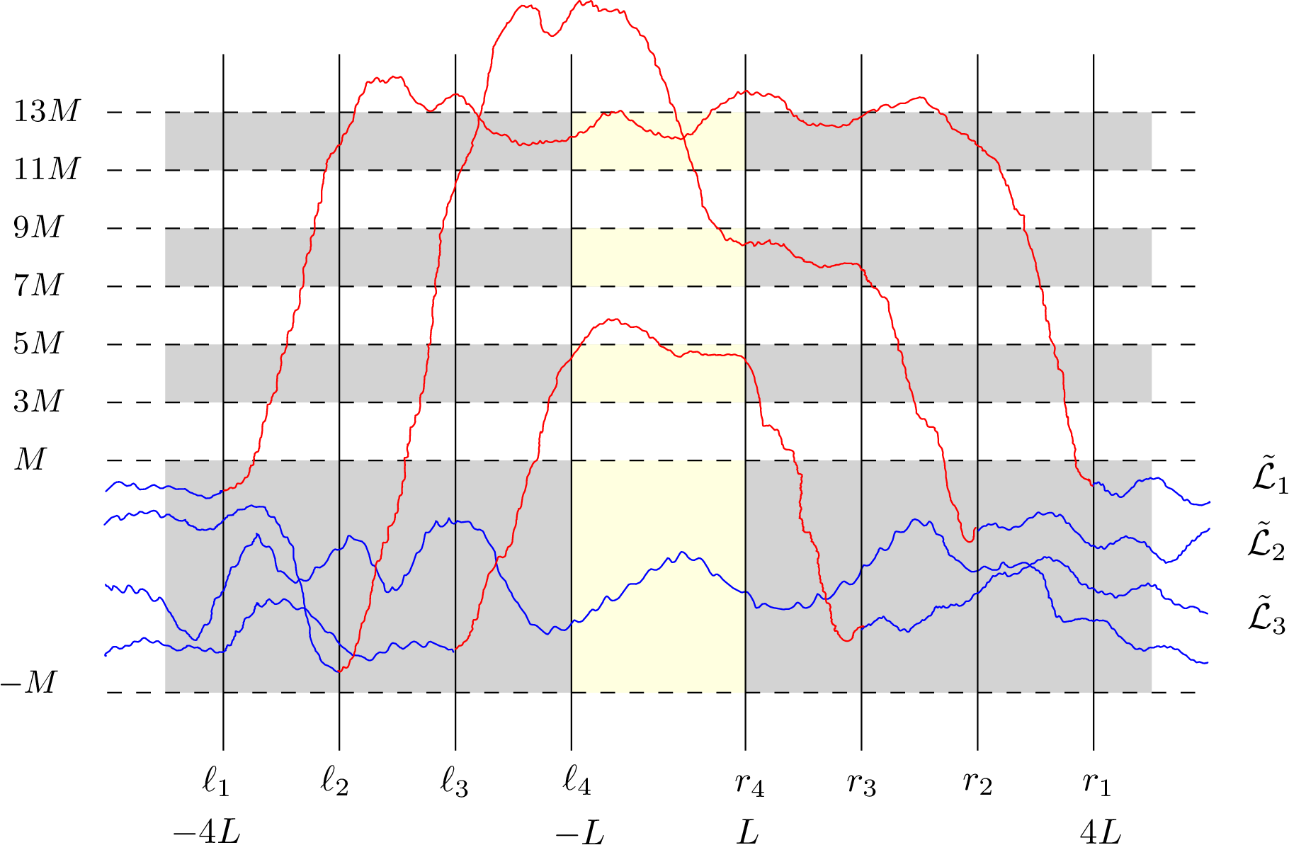
Now we are ready to explain the heuristics of our two-step inductive argument, introduced to resolve the difficulties caused by the intersecting nature of the KPZ line ensemble. To achieve (1.14), we rely on the stochastic monotonicity, Lemma 2.10. The stochastic monotonicity captures the idea that the interaction between ℌ1t\mathfrak{H}^{t}_{1} and ℌ2t\mathfrak{H}^{t}_{2} would push ℌ1t\mathfrak{H}^{t}_{1} upward so ℌ1t\mathfrak{H}^{t}_{1} is more likely to go up. This implies ℌ1t>ℌ2t\mathfrak{H}^{t}_{1}>\mathfrak{H}^{t}_{2} and ℌ1t>ℌ3t\mathfrak{H}^{t}_{1}>\mathfrak{H}^{t}_{3} on [−1,1][-1,1] are plausible to happen. However, because ℌ2t\mathfrak{H}^{t}_{2} is interacting with ℌ1t\mathfrak{H}^{t}_{1} and ℌ3t\mathfrak{H}^{t}_{3} simultaneously, ℌ2t\mathfrak{H}^{t}_{2} does not have a clear tendency. We overcome this difficulty through a novel inductive two-step resampling procedure. The idea is that if ℌ1t\mathfrak{H}^{t}_{1} is very high, ℌ2t\mathfrak{H}^{t}_{2} will almost not be affected by ℌ1t\mathfrak{H}^{t}_{1}. Hence ℌ3t\mathfrak{H}^{t}_{3} can still push ℌ2t\mathfrak{H}^{t}_{2} upward. We can lift ℌ1t\mathfrak{H}^{t}_{1} first and then push ℌ2t\mathfrak{H}^{t}_{2} up. After this step, both ℌ1t\mathfrak{H}^{t}_{1} and ℌ2t\mathfrak{H}^{t}_{2} are larger than ℌ3t\mathfrak{H}^{t}_{3} on [−1,1][-1,1], but ℌ2t≥ℌ1t\mathfrak{H}^{t}_{2}\geq\mathfrak{H}^{t}_{1} could occur. In the second step, we may apply a similar argument in the opposite direction to lower ℌ2t\mathfrak{H}^{t}_{2} because ℌ3t\mathfrak{H}^{t}_{3} is far below. At the end, we can achieve the ordering ℌ1t>ℌ2t>ℌ3t\mathfrak{H}^{t}_{1}>\mathfrak{H}^{t}_{2}>\mathfrak{H}^{t}_{3} on [−1,1][-1,1]. This in particular implies (1.14). See Figure 3 for an illustration.

Refer to caption Refer to caption
Figure 3. An illustration of the two-step inductive argument to separate curves. In the first step, we ensure that ℌ1t>ℌ3t\mathfrak{H}^{t}_{1}>\mathfrak{H}^{t}_{3} and ℌ2t>ℌ3t\mathfrak{H}^{t}_{2}>\mathfrak{H}^{t}_{3} on the interval [−1,1][-1,1]. However, ℌ2t≥ℌ1t\mathfrak{H}^{t}_{2}\geq\mathfrak{H}^{t}_{1} may happen. See the picture on the left. In the second step, we push ℌ3t,ℌ2t\mathfrak{H}^{t}_{3},\mathfrak{H}^{t}_{2} down to ensure ℌ1t>ℌ2t>ℌ3t\mathfrak{H}^{t}_{1}>\mathfrak{H}^{t}_{2}>\mathfrak{H}^{t}_{3} on [−1,1][-1,1]. See the picture on the right.

1.6. Outline

Section 2.1 contains relevant definitions about Gibbsian line ensembles. Section 2.3 contains lemmas about the stochastic monotonicity and the strong Markov property. Main results are stated in Section 1.4 and are proved in Section 3. The main technical result, Proposition 3.1, is proved in Section 4. We also record basic estimates on Brownian bridges in Appendix A and deduce tail estimates for the scaled KPZ line ensembles in Appendix B.

1.7. Notations

We would like to explain some notation here. The natural numbers are defined to be ℕ={1,2,…}.\mathbb{N}=\{1,2,...\}. For integers k1≤k2k_{1}\leq k_{2}, let [k1,k2]ℤ:={k1,k1+1,…,k2}[k_{1},k_{2}]_{\mathbb{Z}}:=\{k_{1},k_{1}+1,\ldots,k_{2}\}. Events are denoted in a special font 𝖤\mathsf{E}, their indicator function is written as 𝟙𝖤\mathbbm{1}_{\mathsf{E}} and their complement is written as 𝖤c\mathsf{E}^{c}.

Universal constants will be generally denoted by CC and constants depending only on kk will be denoted as D=D⁡(k)D=D(k). We label the ones in statements of theorems, lemmas and propositions with subscripts (e.g. D1​(k),D2​(k),⋯D_{1}(k),D_{2}(k),\cdots based on their order of occurrence) but the constants in proofs may change value from line to line.

1.8. Acknowledgment

The author thanks Ivan Corwin for comments concerning a draft version of this paper. The author is grateful for the three Minerva lectures that Alan Hammond has given at Columbia in Spring 2019 on Gibbsian line ensembles.

2. KPZ line ensemble and 𝐇\mathbf{H}-Brownian Gibbs property

In this section we define 𝐇\mathbf{H}-Brownian Gibbsian line ensembles and discuss their properties in Section 2.1 and Section 2.3. The Gibbs property for the KPZ line ensemble is formulated in Section 2.2

2.1. Line ensembles and the 𝐇\mathbf{H}-Brownian Gibbs property

Definition 2.1 (Line ensembles).

Let Σ\Sigma be an interval of ℤ\mathbb{Z} and let Λ\Lambda be a subset of ℝ\mathbb{R}. Consider the set C⁡(Σ×Λ,ℝ)C(\Sigma\times\Lambda,\mathbb{R}) of continuous functions from Σ×Λ\Sigma\times\Lambda to ℝ\mathbb{R} endowed with the topology of uniform convergence on compact subsets of Σ×Λ\Sigma\times\Lambda, and let 𝒞⁡(Σ×Λ,ℝ)\mathcal{C}(\Sigma\times\Lambda,\mathbb{R}) denote the sigma-field generated by Borel sets in C⁡(Σ×Λ,ℝ)C(\Sigma\times\Lambda,\mathbb{R}). A Σ×Λ\Sigma\times\Lambda-indexed line ensemble ℒ\mathcal{L} is a random variable on a probability space (Ω,ℬ,ℙ)(\Omega,\mathcal{B},\mathbb{P}), taking values in C⁡(Σ×Λ,ℝ)C(\Sigma\times\Lambda,\mathbb{R}) such that ℒ\mathcal{L} is a measurable function from ℬ\mathcal{B} to 𝒞⁡(Σ×Λ,ℝ)\mathcal{C}(\Sigma\times\Lambda,\mathbb{R}).

We think of such line ensembles as multi-layer random curves. We will generally write ℒ:Σ×Λ→ℝ\mathcal{L}:\Sigma\times\Lambda\to\mathbb{R} even though it is not ℒ\mathcal{L}, but rather ℒ⁡(ω)\mathcal{L}(\omega) for each ω∈Ω\omega\in\Omega which is such a function. We will also sometimes specify a line ensemble by only giving its law without reference to the underlying probability space. We write ℒi​(⋅):=(ℒ⁡(ω))​(i,⋅)\mathcal{L}_{i}(\cdot):=\big(\mathcal{L}(\omega)\big)(i,\cdot) for the label i∈Σi\in\Sigma curve of the ensemble ℒ\mathcal{L}.

Definition 2.2 (Convergence of line ensembles).

Given a Σ×Λ\Sigma\times\Lambda-indexed line ensemble ℒ\mathcal{L} and a sequence of such ensembles {ℒN}N≥1\left\{\mathcal{L}^{N}\right\}_{N\geq 1}, we will say that ℒN\mathcal{L}^{N} converges to ℒ\mathcal{L} weakly as a line ensemble if for all bounded continuous functions F:C⁡(Σ×Λ,ℝ)→ℝF:C(\Sigma\times\Lambda,\mathbb{R})\to\mathbb{R}, it holds that,

limN→∞∫F⁡(ℒN​(ω))​d​ℙN​(ω)=∫F⁡(ℒ⁡(ω))​𝑑ℙ​(ω).\lim_{N\to\infty}\int F\big(\mathcal{L}^{N}(\omega)\big)d\mathbb{P}^{N}(\omega)=\int F\big(\mathcal{L}(\omega)\big)d\mathbb{P}(\omega).

This is equivalent to weak-∗* convergence in C⁡(Σ×Λ,ℝ)C(\Sigma\times\Lambda,\mathbb{R}) endowed with the topology of uniform convergence on compact subsets of Σ×Λ\Sigma\times\Lambda.

We now start to formulate the 𝐇\mathbf{H}-Brownian Gibbs property. We adopt the convention that all Brownian motions and bridges have diffusion parameter one.

Definition 2.3 (𝐇\mathbf{H}-Brownian bridge line ensemble).

Fix k1≤k2k_{1}\leq k_{2} with k1,k2∈ℤk_{1},k_{2}\in\mathbb{Z}, an interval [a,b]⊂ℝ[a,b]\subset\mathbb{R} and two vectors x→,y→∈ℝk2−k1+1\vec{x},\vec{y}\in\mathbb{R}^{k_{2}-k_{1}+1}. A [k1,k2]ℤ×[a,b][k_{1},k_{2}]_{\mathbb{Z}}\times[a,b]-indexed line ensemble ℒ=(ℒk1,…,ℒk2)\mathcal{L}=(\mathcal{L}_{k_{1}},\ldots,\mathcal{L}_{k_{2}}) is called a free Brownian bridge line ensemble with entrance data x→\vec{x} and exit data y→\vec{y} if its law ℙfreek1,k2,[a,b],x→,y→\mathbb{P}^{k_{1},k_{2},[a,b],\vec{x},\vec{y}}_{\textup{free}} is that of k2−k1+1k_{2}-k_{1}+1 independent standard Brownian bridges starting at time aa at the points x→\vec{x} and ending at time bb at the points y→\vec{y}.

A Hamiltonian 𝐇\mathbf{H} is defined to be a measurable function 𝐇:ℝ→[0,∞]\mathbf{H}:\mathbb{R}\to[0,\infty]. Throughout, we will make use of the special Hamiltonian

(2.1) 𝐇t​(x)=et1/3​x.\displaystyle\mathbf{H}_{t}(x)=e^{t^{1/3}x}.

Fix a Hamiltonian 𝐇\mathbf{H}. Let k1≤k2k_{1}\leq k_{2} be two integers, x→,y→∈ℝk2−k1−1\vec{x},\vec{y}\in\mathbb{R}^{k_{2}-k_{1}-1}, f,g:(a,b)→ℝ∪{±∞}f,g:(a,b)\to\mathbb{R}\cup\{\pm\infty\} be two measurable functions. The Boltzmann weight of ℒ=(ℒk1,ℒk1+1,…,ℒk2)∈C⁡([k1,k2]ℤ×[a,b],ℝ)\mathcal{L}=(\mathcal{L}_{k_{1}},\mathcal{L}_{k_{1}+1},\dots,\mathcal{L}_{k_{2}})\in C([k_{1},k_{2}]_{\mathbb{Z}}\times[a,b],\mathbb{R}) is defined by

(2.2) W𝐇k1,k2,(a,b),x→,y→,f,g(ℒ):=exp{−∑i=k1−1k2∫ab𝐇(ℒi+1(u)−ℒi(u))du},W_{\mathbf{H}}^{k_{1},k_{2},(a,b),\vec{x},\vec{y},f,g}(\mathcal{L}):=\exp\Bigg\{-\sum_{i=k_{1}-1}^{k_{2}}\int_{a}^{b}\mathbf{H}\Big(\mathcal{L}_{i+1}(u)-\mathcal{L}_{i}(u)\Big)du\Bigg\},

where we adopt conventions that ℒk1−1=f\mathcal{L}_{k_{1}-1}=f, ℒk2+1=g\mathcal{L}_{k_{2}+1}=g. The normalizing constant is defined by

(2.3) Z𝐇k1,k2,(a,b),x→,y→,f,g:=𝔼freek1,k2,(a,b),x→,y→​[W𝐇k1,k2,(a,b),x→,y→,f,g​(ℒ)],Z_{\mathbf{H}}^{k_{1},k_{2},(a,b),\vec{x},\vec{y},f,g}:=\mathbb{E}^{k_{1},k_{2},(a,b),\vec{x},\vec{y}}_{\textup{free}}\Big[W_{\mathbf{H}}^{k_{1},k_{2},(a,b),\vec{x},\vec{y},f,g}(\mathcal{L})\Big],

where ℒ\mathcal{L} in the above expectation is distributed according to the measure ℙfreek1,k2,(a,b),x→,y→\mathbb{P}^{k_{1},k_{2},(a,b),\vec{x},\vec{y}}_{\textup{free}}.

Suppose Z𝐇k1,k2,(a,b),x→,y→,f,gZ_{\mathbf{H}}^{k_{1},k_{2},(a,b),\vec{x},\vec{y},f,g} is positive. We define the 𝐇\mathbf{H}-Brownian bridge line ensemble with entrance data x→\vec{x}, exit data y→\vec{y} and boundary data (f,g)(f,g) to be a [k1,k2]ℤ×[a,b][k_{1},k_{2}]_{\mathbb{Z}}\times[a,b]-indexed line ensemble ℒ=(ℒk1,…,ℒk2)\mathcal{L}=(\mathcal{L}_{k_{1}},\ldots,\mathcal{L}_{k_{2}}) with law ℙ𝐇k1,k2,(a,b),x→,y→,f,g\mathbb{P}^{k_{1},k_{2},(a,b),\vec{x},\vec{y},f,g}_{\mathbf{H}} given according to the following Radon-Nikodym derivative relation:

d​ℙ𝐇k1,k2,(a,b),x→,y→,f,gd​ℙfreek1,k2,(a,b),x→,y→​(ℒ):=W𝐇k1,k2,(a,b),x→,y→,f,g​(ℒ)Z𝐇k1,k2,(a,b),x→,y→,f,g.\frac{\textup{d}\mathbb{P}_{\mathbf{H}}^{k_{1},k_{2},(a,b),\vec{x},\vec{y},f,g}}{\textup{d}\mathbb{P}_{\textup{free}}^{k_{1},k_{2},(a,b),\vec{x},\vec{y}}}(\mathcal{L}):=\frac{W_{\mathbf{H}}^{k_{1},k_{2},(a,b),\vec{x},\vec{y},f,g}(\mathcal{L})}{Z_{\mathbf{H}}^{k_{1},k_{2},(a,b),\vec{x},\vec{y},f,g}}.

Moreover, given a′<b′a^{\prime}<b^{\prime} contained in (a,b)(a,b), we define

(2.4) W𝐇,(a′,b′)k1,k2,(a,b),x→,y→,f,g(ℒ):=exp{−∑i=k1−1k2∫[a,a′]∪[b′,b]𝐇(ℒi+1(u)−ℒi(u))du}.W_{\mathbf{H},(a^{\prime},b^{\prime})}^{k_{1},k_{2},(a,b),\vec{x},\vec{y},f,g}(\mathcal{L}):=\exp\Bigg\{-\sum_{i=k_{1}-1}^{k_{2}}\int_{[a,a^{\prime}]\cup[b^{\prime},b]}\mathbf{H}\Big(\mathcal{L}_{i+1}(u)-\mathcal{L}_{i}(u)\Big)du\Bigg\}.

That is, the weight is calculated on [a,a′]∪[b′,b][a,a^{\prime}]\cup[b^{\prime},b] but not on (a′,b′)(a^{\prime},b^{\prime}). We similarly define

(2.5) Z𝐇,(a′,b′)k1,k2,(a,b),x→,y→,f,g:=𝔼freek1,k2,(a,b),x→,y→​[W𝐇,(a′,b′)k1,k2,(a,b),x→,y→,f,g​(ℒ)],Z_{\mathbf{H},(a^{\prime},b^{\prime})}^{k_{1},k_{2},(a,b),\vec{x},\vec{y},f,g}:=\mathbb{E}^{k_{1},k_{2},(a,b),\vec{x},\vec{y}}_{\textup{free}}\Big[W_{\mathbf{H},(a^{\prime},b^{\prime})}^{k_{1},k_{2},(a,b),\vec{x},\vec{y},f,g}(\mathcal{L})\Big],

and

d​ℙ𝐇,(a′,b′)k1,k2,(a,b),x→,y→,f,gd​ℙfreek1,k2,(a,b),x→,y→​(ℒ):=W𝐇,(a′,b′)k1,k2,(a,b),x→,y→,f,g​(ℒ)Z𝐇,(a′,b′)k1,k2,(a,b),x→,y→,f,g.\frac{\textup{d}\mathbb{P}_{\mathbf{H},(a^{\prime},b^{\prime})}^{k_{1},k_{2},(a,b),\vec{x},\vec{y},f,g}}{\textup{d}\mathbb{P}_{\textup{free}}^{k_{1},k_{2},(a,b),\vec{x},\vec{y}}}(\mathcal{L}):=\frac{W_{\mathbf{H},(a^{\prime},b^{\prime})}^{k_{1},k_{2},(a,b),\vec{x},\vec{y},f,g}(\mathcal{L})}{Z_{\mathbf{H},(a^{\prime},b^{\prime})}^{k_{1},k_{2},(a,b),\vec{x},\vec{y},f,g}}.

𝐇\mathbf{H}-Brownian Gibbs property could be viewed as a spatial Markov property, more specifically, it provides a description of the conditional law inside a compact set.

Definition 2.4 (𝐇\mathbf{H}-Brownian Gibbs property).

Let 𝐇\mathbf{H} be a Hamiltonian, Σ\Sigma be an interval of ℤ\mathbb{Z} and Λ\Lambda be a subset of ℝ\mathbb{R}. A Σ×Λ\Sigma\times\Lambda-indexed line ensemble ℒ\mathcal{L} satisfies the 𝐇\mathbf{H}-Brownian Gibbs property if the following holds. For all [k1,k2]ℤ⊂Σ[k_{1},k_{2}]_{\mathbb{Z}}\subset\Sigma and [a,b]⊂Λ[a,b]\subset\Lambda, set x→=(ℒk1​(a),⋯,ℒk2​(a))\vec{x}=\big(\mathcal{L}_{k_{1}}(a),\cdots,\mathcal{L}_{k_{2}}(a)\big), y→=(ℒk1​(b),…,ℒk2​(b))\vec{y}=\big(\mathcal{L}_{k_{1}}(b),\ldots,\mathcal{L}_{k_{2}}(b)\big), f=ℒk1−1f=\mathcal{L}_{k_{1}-1} and g=ℒk2+1g=\mathcal{L}_{k_{2}+1} with the convention that if k1−1∉Σk_{1}-1\notin\Sigma then f≡+∞f\equiv+\infty and likewise if k2+1∉Σk_{2}+1\notin\Sigma then g≡−∞g\equiv-\infty. Then it holds almost surely that Z𝐇k1,k2,(a,b),x→,y→,f,g>0Z_{\mathbf{H}}^{k_{1},k_{2},(a,b),\vec{x},\vec{y},f,g}>0. Moreover,

(2.6) Law​(ℒ​|conditional on [k1,k2]ℤ×[a,b]​ℒ|(Σ×Λ)∖([k1,k2]ℤ×(a,b)))=ℙ𝐇k1,k2,(a,b),x→,y→,f,g\textrm{Law}\left(\mathcal{L}\left|{}_{[k_{1},k_{2}]_{\mathbb{Z}}\times[a,b]}\ \textrm{conditional on }\mathcal{L}\right|_{(\Sigma\times\Lambda)\setminus([k_{1},k_{2}]_{\mathbb{Z}}\times(a,b))}\right)=\mathbb{P}_{\mathbf{H}}^{k_{1},k_{2},(a,b),\vec{x},\vec{y},f,g}

The following equality (2.7) is an equivalent formulation of (2.6) and it is convenient for computations. For any bounded measurable function FF from C⁡([k1,k2]ℤ×[a,b],ℝ)C\left([k_{1},k_{2}]_{\mathbb{Z}}\times[a,b],\mathbb{R}\right) to ℝ\mathbb{R}, it holds almost surely that

(2.7) 𝔼[F(ℒ|[k1,k2]ℤ×[a,b])|ℱext([k1,k2]ℤ×(a,b))]=𝔼𝐇k1,k2,(a,b),x→,y→,f,g[F(ℒ~)],\mathbb{E}\left[F(\mathcal{L}\big|_{[k_{1},k_{2}]_{\mathbb{Z}}\times[a,b]})\right|\mathcal{F}_{\textrm{ext}}\big([k_{1},k_{2}]_{\mathbb{Z}}\times(a,b)\big)\Big]=\mathbb{E}_{\mathbf{H}}^{k_{1},k_{2},(a,b),\vec{x},\vec{y},f,g}\left[F(\tilde{\mathcal{L}})\right],

where

ℱext([k1,k2]ℤ×(a,b)):=σ(ℒi(s):(i,s)∈Σ×Λ∖[k1,k2]ℤ×(a,b))\mathcal{F}_{\textrm{ext}}\left([k_{1},k_{2}]_{\mathbb{Z}}\times(a,b)\right):=\sigma\left(\mathcal{L}_{i}(s):(i,s)\in\Sigma\times\Lambda\setminus[k_{1},k_{2}]_{\mathbb{Z}}\times(a,b)\right)

is the exterior sigma-field generated by the line ensemble outside [k1,k2]ℤ×(a,b)[k_{1},k_{2}]_{\mathbb{Z}}\times(a,b). On the right-hand side ℒ~\tilde{\mathcal{L}} is distributed according to ℙ𝐇k1,k2,(a,b),x→,y→,f,g\mathbb{P}_{\mathbf{H}}^{k_{1},k_{2},(a,b),\vec{x},\vec{y},f,g}.

Definition 2.5.

Consider the following special Hamiltonian,

𝐇ord​(x)={+∞,x>0,0,x≤0,\mathbf{H}_{\textup{ord}}(x)=\left\{\begin{array}[]{cc}+\infty,&x>0,\\ 0,&x\leq 0,\end{array}\right.

Its corresponding 𝐇ord\mathbf{H}_{\textup{ord}}-Brownian Gibbs property was also referred to as Brownian Gibbs property [CH14]. The reason is that 𝐇ord\mathbf{H}_{\textup{ord}}-Brownian bridge line ensemble (defined in Definition 2.3) is non-intersecting Brownian bridges conditioned on avoiding the upper and lower boundaries. We note that a Brownian Gibbsian line ensemble must be ordered with probability one.

2.2. Gibbs property of the KPZ line ensemble

For t>0t>0, recall that the KPZ line ensemble ℋt\mathcal{H}^{t} is a ℕ×ℝ\mathbb{N}\times\mathbb{R}-indexed line ensemble defined in Definition 1.1. The Gibbs property of ℋt\mathcal{H}^{t} is proved in [CH16, Theorem 2.15] and we record it as the theorem below.

Theorem 2.6.

For any t>0t>0, the KPZ line ensemble ℋt\mathcal{H}^{t} satisfies the 𝐇\mathbf{H}-Brownian Gibbs property with 𝐇⁡(x)=ex\mathbf{H}(x)=e^{x}.

We are mostly interested in the scaled KPZ line ensemble ℌt\mathfrak{H}^{t} defined in Definition 1.2. Recall 𝐇t​(x)=et1/3​x.\mathbf{H}_{t}(x)=e^{t^{1/3}x}. Through a direct computation we have the following corollary.

Corollary 2.7.

For any t>0t>0, the line ensemble ℌt{\mathfrak{H}}^{t} satisfies the 𝐇t\mathbf{H}_{t}-Brownian Gibbs property.

2.3. Strong Gibbs property and stochastic monotonicity

We record some important properties, developed in [CH16, Section 2], about 𝐇\mathbf{H}-Gibbsian line ensembles in this section. We begin with the strong Gibbs property, which enables us to resample the trajectory within a stopping domain as opposed to a deterministic interval.

Definition 2.8.

Let Σ\Sigma be an interval of ℤ\mathbb{Z}, and Λ\Lambda be an interval of ℝ\mathbb{R}. Consider a Σ×Λ\Sigma\times\Lambda-indexed line ensemble ℒ\mathcal{L} which has the 𝐇\mathbf{H}-Brownian Gibbs property for some Hamiltonian 𝐇\mathbf{H}. For [k1,k2]ℤ⊆Σ[k_{1},k_{2}]_{\mathbb{Z}}\subseteq\Sigma and (ℓ,r)⊆Λ(\ell,r)\subseteq\Lambda, ℱext​([k1,k2]ℤ×(ℓ,r))\mathcal{F}_{\textrm{ext}}\big([k_{1},k_{2}]_{\mathbb{Z}}\times(\ell,r)\big) denotes the sigma-field generated by the data outside [k1,k2]ℤ×(ℓ,r)[k_{1},k_{2}]_{\mathbb{Z}}\times(\ell,r). The random variable (𝔩,𝔯)(\mathfrak{l},\mathfrak{r}) is called a [k1,k2]ℤ[k_{1},k_{2}]_{\mathbb{Z}}-stopping domain if for all ℓ<r\ell<r,

{𝔩≤ℓ,𝔯≥r}∈ℱext​([k1,k2]ℤ×(ℓ,r)).\big\{\mathfrak{l}\leq\ell,\mathfrak{r}\geq r\big\}\in\mathcal{F}_{\textrm{ext}}\big([k_{1},k_{2}]_{\mathbb{Z}}\times(\ell,r)\big).

For [k1,k2]ℤ⊂ℤ[k_{1},k_{2}]_{\mathbb{Z}}\subset\mathbb{Z}, define

Ck1,k2:={(ℓ,r,f):ℓ<r,f=(fk1,…,fk2)∈C([k1,k2]ℤ×[ℓ,r])}.\displaystyle C^{k_{1},k_{2}}:=\left\{(\ell,r,f)\,:\,\ell<r,\ f=(f_{k_{1}},\dots,f_{k_{2}})\in C([k_{1},k_{2}]_{\mathbb{Z}}\times[\ell,r])\right\}.
Lemma 2.9.

Consider a Σ×Λ\Sigma\times\Lambda-indexed line ensemble ℒ\mathcal{L} which has the 𝐇\mathbf{H}-Brownian Gibbs property. Fix [k1,k2]ℤ⊆Σ[k_{1},k_{2}]_{\mathbb{Z}}\subseteq\Sigma. For all random variables (𝔩,𝔯)(\mathfrak{l},\mathfrak{r}) which are [k1,k2]ℤ[k_{1},k_{2}]_{\mathbb{Z}}-stopping domains for ℒ\mathcal{L}, the following strong 𝐇\mathbf{H}-Brownian Gibbs property holds: for all Borel functions F:Ck1,k2→ℝF:C^{k_{1},k_{2}}\to\mathbb{R}, ℙ\mathbb{P}-almost surely,

(2.8) 𝔼⁡[F⁡(𝔩,𝔯,ℒ|[k1,k2]ℤ×[𝔩,𝔯])|ℱext​([k1,k2]ℤ×(𝔩,𝔯))]=𝔼𝐇k1,k2,(𝔩,𝔯),x→,y→,f,g​[F⁡(𝔩,𝔯,ℒ~)],\mathbb{E}\bigg[F\Big(\mathfrak{l},\mathfrak{r},\mathcal{L}\big|_{[k_{1},k_{2}]_{\mathbb{Z}}\times[\mathfrak{l},\mathfrak{r}]}\Big)\Big|\mathcal{F}_{\textrm{ext}}\big([k_{1},k_{2}]_{\mathbb{Z}}\times(\mathfrak{l},\mathfrak{r})\big)\bigg]=\mathbb{E}^{k_{1},k_{2},(\mathfrak{l},\mathfrak{r}),\vec{x},\vec{y},f,g}_{\mathbf{H}}\Big[F\big(\mathfrak{l},\mathfrak{r},\tilde{\mathcal{L}})\Big],

where x→={ℒi​(𝔩)}i=k1k2\vec{x}=\{\mathcal{L}_{i}(\mathfrak{l})\}_{i=k_{1}}^{k_{2}}, y→={ℒi​(𝔯)}i=k1k2\vec{y}=\{\mathcal{L}_{i}(\mathfrak{r})\}_{i=k_{1}}^{k_{2}}, f=ℒk1−1f=\mathcal{L}_{k_{1}-1} (or ∞\infty if k1−1∉Σk_{1}-1\notin\Sigma), g=ℒk2+1g=\mathcal{L}_{k_{2}+1} (or −∞-\infty if k2+1∉Σk_{2}+1\notin\Sigma). On the left-hand side ℒ|[k1,k2]ℤ×[𝔩,𝔯]\mathcal{L}\big|_{[k_{1},k_{2}]_{\mathbb{Z}}\times[\mathfrak{l},\mathfrak{r}]} is the restriction of curves distributed according to the law of ℒ\mathcal{L} and on the right-hand side ℒ~\tilde{\mathcal{L}} is distributed according to ℙ𝐇k1,k2,(𝔩,𝔯),x→,y→,f,g\mathbb{P}^{k_{1},k_{2},(\mathfrak{l},\mathfrak{r}),\vec{x},\vec{y},f,g}_{\mathbf{H}}.

For a convex Hamiltonian 𝐇\mathbf{H} (such as 𝐇t\mathbf{H}_{t}), 𝐇\mathbf{H}-Brownian bridge line ensembles enjoy stochastic monotonicity.

Lemma 2.10.

Fix k1≤k2k_{1}\leq k_{2} with k1,k2∈ℤk_{1},k_{2}\in\mathbb{Z} and [a,b]⊂ℝ[a,b]\subset\mathbb{R}. Consider two pairs of vectors x→(i),y→(i)∈ℝk2−k1+1\vec{x}^{(i)},\vec{y}^{(i)}\in\mathbb{R}^{k_{2}-k_{1}+1} and two pairs of measurable functions (f(i),g(i))(f^{(i)},g^{(i)}) for i∈{1,2}i\in\{1,2\} such that xj(1)≤xj(2)x^{(1)}_{j}\leq x^{(2)}_{j} and yj(1)≤yj(2)y^{(1)}_{j}\leq y^{(2)}_{j} for all j∈[k1,k2]ℤj\in[k_{1},k_{2}]_{\mathbb{Z}} and f(1)​(u)≤f(2)​(u),g(1)​(u)≤g(2)​(u)f^{(1)}(u)\leq f^{(2)}(u),g^{(1)}(u)\leq g^{(2)}(u) for all u∈(a,b)u\in(a,b). Suppose that Z𝐇k1,k2,(a,b),x→(i),y→(i),f(i),g(i)>0Z_{\mathbf{H}}^{k_{1},k_{2},(a,b),\vec{x}^{(i)},\vec{y}^{(i)},f^{(i)},g^{(i)}}>0 for i∈{1,2}i\in\{1,2\}. Let 𝒬(i)={𝒬k(i),…,𝒬k2(i)}\mathcal{Q}^{(i)}=\{\mathcal{Q}^{(i)}_{k},\dots,\mathcal{Q}^{(i)}_{k_{2}}\} be a [k1,k2]ℤ×[a,b][k_{1},k_{2}]_{\mathbb{Z}}\times[a,b]-indexed line ensemble with law ℙ𝐇k1,k2,(a,b),x→(i),y→(i),f(i),g(i)\mathbb{P}_{\mathbf{H}}^{k_{1},k_{2},(a,b),\vec{x}^{(i)},\vec{y}^{(i)},f^{(i)},g^{(i)}}. See Definition 2.3.

If the Hamiltonian 𝐇\mathbf{H} is convex, then there exists a coupling of 𝒬(1)\mathcal{Q}^{(1)} and 𝒬(2)\mathcal{Q}^{(2)} such that almost surely 𝒬j(1)​(u)≤𝒬j(2)​(u)\mathcal{Q}^{(1)}_{j}(u)\leq\mathcal{Q}^{(2)}_{j}(u) for all (j,u)∈[k1,k2]ℤ×[a,b](j,u)\in[k_{1},k_{2}]_{\mathbb{Z}}\times[a,b].

3. Proof of main results

In this section we prove Theorem 1.4 and Theorem 1.5. The proofs rely heavily on the key technical result, Proposition 3.1, which provides a quantitative lower bound on the normalization constant ZZ. We state Proposition 3.1 below and postpone its proof to the next section.

Proposition 3.1.

Fix k∈ℕk\in\mathbb{N} and L≥1L\geq 1. There exists a constant D1=D1​(k)D_{1}=D_{1}(k) depending only on kk such that the following statement holds. For all t≥1t\geq 1 and K≥L2K\geq L^{2}, we have

(3.1) ℙ⁡(Z𝐇t1,k,(−L,L),x→,y→,+∞,ℌk+1t<D1−1​e−D1​L−1​K2)<e−K3/2,\displaystyle\mathbb{P}\left(Z^{1,k,(-L,L),\vec{x},\vec{y},+\infty,\mathfrak{H}^{t}_{k+1}}_{\mathbf{H}_{t}}<D_{1}^{-1}e^{-D_{1}L^{-1}K^{2}}\right)<e^{-K^{3/2}},

where x→=(ℌit​(−L))i=1k\vec{x}=\big(\mathfrak{H}^{t}_{i}(-L)\big)_{i=1}^{k} and y→=(ℌit​(L))i=1k\vec{y}=\big(\mathfrak{H}^{t}_{i}(L)\big)_{i=1}^{k}.

3.1. Proof of Theorem 1.4 and Theorem 1.5(i)

We begin with proving Theorem 1.4.

Proof of Theorem 1.4.

Fix L=1L=1 and ε∈(0,e−1]\varepsilon\in(0,e^{-1}]. We will exploit Gibbs resampling on [1,k]ℤ×[−1,1][1,k]_{\mathbb{Z}}\times[-1,1]. We start with controlling the boundary values ℌkt​(±1)\mathfrak{H}^{t}_{k}(\pm 1). Let D′=max⁡{D9,D10}D^{\prime}=\max\{D_{9},D_{10}\} with D9,D10D_{9},D_{10} from Proposition B.1 and Proposition B.2. Set

r:=(D′​log⁡ε−1+D′​log⁡(2​D′))2/3r:=\left(D^{\prime}\log\varepsilon^{-1}+D^{\prime}\log(2D^{\prime})\right)^{2/3}

and denote

𝖤1:={supu∈[−1,1]|ℌkt(u)+2−1u2|<r}.\mathsf{E}_{1}:=\left\{\sup_{u\in[-1,1]}\left|\mathfrak{H}^{t}_{k}(u)+2^{-1}u^{2}\right|<r\right\}.

By the tail estimates in Proposition B.1 and Proposition B.2, we have ℙ⁡(𝖤1c)<ε\mathbb{P}(\mathsf{E}_{1}^{c})<\varepsilon.
Recall the convention that x→=(ℌit​(−L))i=1k\vec{x}=\big(\mathfrak{H}^{t}_{i}(-L)\big)_{i=1}^{k} and y→=(ℌit​(L))i=1k\vec{y}=\big(\mathfrak{H}^{t}_{i}(L)\big)_{i=1}^{k} and denote

𝖤2:={Z𝐇t1,k,(−1,1),x→,y→,+∞,ℌk+1t≥δ}.\displaystyle\mathsf{E}_{2}:=\left\{Z^{1,k,(-1,1),\vec{x},\vec{y},+\infty,\mathfrak{H}^{t}_{k+1}}_{\mathbf{H}_{t}}\geq\delta\right\}.

Here δ\delta is a small constant to be determined soon. Let D1D_{1} be the constant in Proposition 3.1. Apply Proposition 3.1 with L=1L=1 and the right hand side being ε∈(0,e−1]\varepsilon\in(0,e^{-1}]. It is easy to check that ℙ⁡(𝖤2c)<ε\mathbb{P}(\mathsf{E}_{2}^{c})<\varepsilon by picking

(3.2) δ:=\displaystyle\delta:= D1−1​e−D1​(log⁡ε−1)4/3.\displaystyle D_{1}^{-1}e^{-D_{1}(\log\varepsilon^{-1})^{4/3}}.

Let B:[−1,1]→ℝB:[-1,1]\to\mathbb{R} be a free Brownian bridge with B⁡(±1)=0B(\pm 1)=0 and write ℙfree\mathbb{P}_{\textup{free}} to represent the law of BB. Let C0C_{0} be the universal constant in Lemma A.2. For all K≥0K\geq 0 and all d∈(0,1]d\in(0,1],

ℙfree​(supu,v∈[0,d]|B⁡(u)−B⁡(v)|≥K​d1/2)≤C0​e−C0−1​K2.\displaystyle\mathbb{P}_{\textup{free}}\left(\sup_{u,v\in[0,d]}\left|B(u)-B(v)\right|\geq Kd^{1/2}\right)\leq C_{0}e^{-C_{0}^{-1}K^{2}}.

Define K=K⁡(ε)K=K(\varepsilon) as

(3.3) K⁡(ε):=max⁡{2​r,(8​C0​D1)1/2​(log⁡ε−1)2/3}.\displaystyle K(\varepsilon):=\max\{2r,(8C_{0}D_{1})^{1/2}\left(\log\varepsilon^{-1}\right)^{2/3}\}.

Let

ℌkt,[−1,1]​(u):=ℌkt​(u)−(2−1​(1−u)​ℌkt​(−1)+2−1​(u−1)​ℌkt​(1)).\displaystyle\mathfrak{H}^{t,[-1,1]}_{k}(u):=\mathfrak{H}^{t}_{k}(u)-\left(2^{-1}(1-u)\mathfrak{H}^{t}_{k}(-1)+2^{-1}(u-1)\mathfrak{H}^{t}_{k}(1)\right).

Define the events

𝖦≔\displaystyle\mathsf{G}\coloneqq {supu,v∈[0,d]|ℌkt(u)−ℌkt(v)|≥Kd1/2}\displaystyle\left\{\sup_{u,v\in[0,d]}\left|\mathfrak{H}_{k}^{t}(u)-\mathfrak{H}_{k}^{t}(v)\right|\geq Kd^{1/2}\right\}
𝖦′≔\displaystyle\mathsf{G}^{\prime}\coloneqq {supu,v∈[0,d]|ℌkt,[−1,1](u)−ℌkt,[−1,1](v)|≥2−1Kd1/2}.\displaystyle\left\{\sup_{u,v\in[0,d]}\left|\mathfrak{H}_{k}^{t,[-1,1]}(u)-\mathfrak{H}_{k}^{t,[-1,1]}(v)\right|\geq 2^{-1}Kd^{1/2}\right\}.

Note that

supu,v∈[0,d]|ℌkt​(u)−ℌkt​(v)|≤supu,v∈[0,d]|ℌkt,[−1,1]​(u)−ℌkt,[−1,1]​(v)|+2−1​d​|ℌkt​(1)−ℌkt​(−1)|.\displaystyle\sup_{u,v\in[0,d]}\left|\mathfrak{H}_{k}^{t}(u)-\mathfrak{H}_{k}^{t}(v)\right|\leq\sup_{u,v\in[0,d]}\left|\mathfrak{H}_{k}^{t,[-1,1]}(u)-\mathfrak{H}_{k}^{t,[-1,1]}(v)\right|+2^{-1}d|\mathfrak{H}_{k}^{t}(1)-\mathfrak{H}_{k}^{t}(-1)|.

When 𝖤1\mathsf{E}_{1}, we have ,

2−1​d​|ℌkt​(1)−ℌkt​(−1)|≤r​d≤r​d1/2.2^{-1}d|\mathfrak{H}_{k}^{t}(1)-\mathfrak{H}_{k}^{t}(-1)|\leq rd\leq rd^{1/2}.

Here we used d≤1d\leq 1. Because K≥2​rK\geq 2r, we deduce that

2−1​d​|ℌkt​(1)−ℌkt​(−1)|≤2−1​K​d1/2.2^{-1}d|\mathfrak{H}_{k}^{t}(1)-\mathfrak{H}_{k}^{t}(-1)|\leq 2^{-1}Kd^{1/2}.

Therefore we have 𝖦∩𝖤1⊂𝖦′∩𝖤1\mathsf{G}\cap\mathsf{E}_{1}\subset\mathsf{G}^{\prime}\cap\mathsf{E}_{1}. Applying the Gibbs property (see Definition 2.4 and Corollary 2.7), we obtain that

𝟙𝖤1∩𝖤2⋅𝔼⁡[𝟙𝖦′|ℱe​x​t​([1,k]ℤ×(−1,1))]=𝟙𝖤1∩𝖤2⋅𝔼free1,k,(−1,1),x→,y→​[𝟙𝖦′⋅W𝐇t1,k,(−1,1),x→,y→,+∞,ℌk+1t]Z𝐇t1,k,(−1,1),x→,y→,+∞,ℌk+1t.\displaystyle\mathbbm{1}_{\mathsf{E}_{1}\cap\mathsf{E}_{2}}\cdot\mathbb{E}[\mathbbm{1}_{\mathsf{G}^{\prime}}\,|\,\mathcal{F}_{{ext}}([1,k]_{\mathbb{Z}}\times(-1,1))]=\mathbbm{1}_{\mathsf{E}_{1}\cap\mathsf{E}_{2}}\cdot\frac{\mathbb{E}^{1,k,(-1,1),\vec{x},\vec{y}}_{\textup{free}}[\mathbbm{1}_{\mathsf{G}^{\prime}}\cdot W^{1,k,(-1,1),\vec{x},\vec{y},+\infty,\mathfrak{H}_{k+1}^{t}}_{\mathbf{H}_{t}}]}{Z^{1,k,(-1,1),\vec{x},\vec{y},+\infty,\mathfrak{H}_{k+1}^{t}}_{\mathbf{H}_{t}}}.

As 𝖤2\mathsf{E}_{2} occurs, Z𝐇t1,k,(−1,1),x→,y→,+∞,ℌk+1t≥δZ^{1,k,(-1,1),\vec{x},\vec{y},+\infty,\mathfrak{H}_{k+1}^{t}}_{\mathbf{H}_{t}}\geq\delta. Together with W𝐇t1,k,(−1,1),x→,y→,+∞,ℌk+1t≤1W^{1,k,(-1,1),\vec{x},\vec{y},+\infty,\mathfrak{H}_{k+1}^{t}}_{\mathbf{H}_{t}}\leq 1, we deduce

𝟙𝖤1∩𝖤2⋅𝔼⁡[𝟙𝖦′|ℱe​x​t​([1,k]ℤ×(−1,1))]\displaystyle\mathbbm{1}_{\mathsf{E}_{1}\cap\mathsf{E}_{2}}\cdot\mathbb{E}[\mathbbm{1}_{\mathsf{G}^{\prime}}\,|\,\mathcal{F}_{{ext}}([1,k]_{\mathbb{Z}}\times(-1,1))] ≤δ−1​ℙfree1,k,(−1,1),x→,y→​(𝖦′)⋅𝟙𝖤1∩𝖤2\displaystyle\leq\delta^{-1}\mathbb{P}^{1,k,(-1,1),\vec{x},\vec{y}}_{\textup{free}}(\mathsf{G}^{\prime})\cdot\mathbbm{1}_{\mathsf{E}_{1}\cap\mathsf{E}_{2}}
≤δ−1​C0​e−4−1​C0−1​K2⋅𝟙𝖤1∩𝖤2.\displaystyle\leq\delta^{-1}C_{0}e^{-4^{-1}C_{0}^{-1}K^{2}}\cdot\mathbbm{1}_{\mathsf{E}_{1}\cap\mathsf{E}_{2}}.

In summary, we obtain that

ℙ⁡(𝖦)\displaystyle\mathbb{P}(\mathsf{G}) ≤ℙ⁡(𝖦∩𝖤1∩𝖤2)+ℙ⁡(𝖤1c)+ℙ⁡(𝖤2c)≤ℙ⁡(𝖦′∩𝖤1∩𝖤2)+ℙ⁡(𝖤1c)+ℙ⁡(𝖤2c)\displaystyle\leq\mathbb{P}(\mathsf{G}\cap\mathsf{E}_{1}\cap\mathsf{E}_{2})+\mathbb{P}(\mathsf{E}_{1}^{\textup{c}})+\mathbb{P}(\mathsf{E}_{2}^{\textup{c}})\leq\mathbb{P}(\mathsf{G}^{\prime}\cap\mathsf{E}_{1}\cap\mathsf{E}_{2})+\mathbb{P}(\mathsf{E}_{1}^{\textup{c}})+\mathbb{P}(\mathsf{E}_{2}^{\textup{c}})
=𝔼⁡[𝟙𝖤1∩𝖤2⋅𝔼⁡[𝟙𝖦′|ℱe​x​t​([1,k]ℤ×(−1,1))]]+ℙ⁡(𝖤1c)+ℙ⁡(𝖤2c)\displaystyle=\mathbb{E}[\mathbbm{1}_{\mathsf{E}_{1}\cap\mathsf{E}_{2}}\cdot\mathbb{E}[\mathbbm{1}_{\mathsf{G}^{\prime}}\,|\,\mathcal{F}_{{ext}}([1,k]_{\mathbb{Z}}\times(-1,1))]]+\mathbb{P}(\mathsf{E}_{1}^{\textup{c}})+\mathbb{P}(\mathsf{E}_{2}^{\textup{c}})
≤δ−1​C0​e−4−1​C0−1​K2+2​ε.\displaystyle\leq\delta^{-1}C_{0}e^{-4^{-1}C_{0}^{-1}K^{2}}+2\varepsilon.

Recall definitions of δ\delta in (3.2) and KK in (3.3), it is easily checked that δ−1≤D1​e8−1​C0−1​K2\delta^{-1}\leq D_{1}e^{8^{-1}C_{0}^{-1}K^{2}}. Moreover there exists D=D⁡(k)D=D(k) such that K≤D2/3​(log⁡ε−1)2/3K\leq D^{2/3}\left(\log\varepsilon^{-1}\right)^{2/3}. Hence we obtain that

ℙ⁡(𝖦)\displaystyle\mathbb{P}\left(\mathsf{G}\right) ≤C0​D1​e−8−1​C0−1​K2+2​ε\displaystyle\leq C_{0}D_{1}e^{-8^{-1}C_{0}^{-1}K^{2}}+2\varepsilon
≤C0​D1​e−8−1​C0−1​K2+2​e−D−1​K3/2\displaystyle\leq C_{0}D_{1}e^{-8^{-1}C_{0}^{-1}K^{2}}+2e^{-D^{-1}K^{3/2}}
≤C0​D1​e−8−1​C0−1​K3/2+2​e−D−1​K3/2.\displaystyle\leq C_{0}D_{1}e^{-8^{-1}C_{0}^{-1}K^{3/2}}+2e^{-D^{-1}K^{3/2}}.

Picking D0​(k)=2​max⁡{C0​D1,8​C0,D,2}D_{0}(k)=2\max\left\{C_{0}D_{1},8C_{0},D,2\right\}, we have

ℙ⁡(𝖦)\displaystyle\mathbb{P}(\mathsf{G}) ≤12​D0​e−D0−1​K3/2+12​D0​e−D0−1​K3/2≤D0​e−D0−1​K3/2.\displaystyle\leq\frac{1}{2}D_{0}e^{-D_{0}^{-1}K^{3/2}}+\frac{1}{2}D_{0}e^{-D_{0}^{-1}K^{3/2}}\leq D_{0}e^{-D_{0}^{-1}K^{3/2}}.

The proof is finished. ∎

Using an union bound argument, we obtain the following corollary.

Corollary 3.2.

Fix k∈ℕk\in\mathbb{N}, L≥1L\geq 1 and d∈(0,1]d\in(0,1]. There exists a constant D2=D2​(k)D_{2}=D_{2}(k) depending only on kk such that the following statement holds. Suppose that K≥4​L​d1/2K\geq 4Ld^{1/2}, then for all t≥1t\geq 1,

ℙ⁡(supu,v∈[−L,L],|u−v|≤d|ℌkt​(u)−ℌkt​(v)|≥K​d1/2)≤d−1​L​D2​e−D2−1​K3/2.\displaystyle\mathbb{P}\left(\sup_{u,v\in[-L,L],\ |u-v|\leq d}\left|\mathfrak{H}_{k}^{t}(u)-\mathfrak{H}_{k}^{t}(v)\right|\geq Kd^{1/2}\right)\leq d^{-1}LD_{2}e^{-D_{2}^{-1}K^{3/2}}.
Proof.

Because

{supu,v∈[−L,L],|u−v|≤d|ℌkt(u)−ℌkt(v)|≥Kd1/2}⊂{supu,v∈[−L,L],|u−v|≤2−1​d|ℌkt(u)−ℌkt(v)|≥2−1Kd1/2},\displaystyle\left\{\sup_{u,v\in[-L,L],\ |u-v|\leq d}\left|\mathfrak{H}_{k}^{t}(u)-\mathfrak{H}_{k}^{t}(v)\right|\geq Kd^{1/2}\right\}\subset\left\{\sup_{u,v\in[-L,L],\ |u-v|\leq 2^{-1}d}\left|\mathfrak{H}_{k}^{t}(u)-\mathfrak{H}_{k}^{t}(v)\right|\geq 2^{-1}Kd^{1/2}\right\},

it suffices to prove the assertion for d≤2−1d\leq 2^{-1}. From now on we assume d∈(0,2−1]d\in(0,2^{-1}].

Let m=⌈d−1​L⌉m=\lceil d^{-1}L\rceil. For j∈[−m,m]ℤj\in[-m,m]_{\mathbb{Z}}, define

𝖤j:={|ℌkt​(u)−ℌkt​(v)|≥K​d1/2​for some​u,v∈[j​d,(j+2)​d]}.\displaystyle\mathsf{E}_{j}:=\left\{\left|\mathfrak{H}_{k}^{t}(u)-\mathfrak{H}_{k}^{t}(v)\right|\geq Kd^{1/2}\,\,\textup{for some}\ u,v\in[jd,(j+2)d]\right\}.

Note that

{supu,v∈[−L,L],|u−v|≤d|ℌkt(u)−ℌkt(v)|≥Kd1/2}⊂⋃j=−mm𝖤j.\displaystyle\left\{\sup_{u,v\in[-L,L],\ |u-v|\leq d}\left|\mathfrak{H}_{k}^{t}(u)-\mathfrak{H}_{k}^{t}(v)\right|\geq Kd^{1/2}\right\}\subset\bigcup_{j={-m}}^{m}\mathsf{E}_{j}.

Fix j∈[−m,m]ℤj\in[-m,m]_{\mathbb{Z}}. By stationarity of ℌkt​(u)+2−1​u2\mathfrak{H}^{t}_{k}(u)+2^{-1}u^{2}, ℌkt​(u)​=(d)​ℌkt​(u−T)−T⁡(u−T)−2−1​T2\mathfrak{H}^{t}_{k}(u)\overset{(d)}{=}\mathfrak{H}^{t}_{k}(u-T)-T(u-T)-2^{-1}T^{2} as a process in uu for any T∈ℝT\in\mathbb{R}. Therefore,

ℙ⁡(𝖤j)=\displaystyle\mathbb{P}(\mathsf{E}_{j})= ℙ⁡(supu,v∈[0,2​d]|ℌkt​(u)−ℌkt​(v)−j​d​(u−v)|≥K​d1/2)\displaystyle\mathbb{P}\left(\sup_{u,v\in[0,2d]}\left|\mathfrak{H}^{t}_{k}(u)-\mathfrak{H}^{t}_{k}(v)-jd(u-v)\right|\geq Kd^{1/2}\right)
≤\displaystyle\leq ℙ⁡(supu,v∈[0,2​d]|ℌkt​(u)−ℌkt​(v)|≥K​d1/2−d⁡(L+1))\displaystyle\mathbb{P}\left(\sup_{u,v\in[0,2d]}\left|\mathfrak{H}^{t}_{k}(u)-\mathfrak{H}^{t}_{k}(v)\right|\geq Kd^{1/2}-d(L+1)\right)
≤\displaystyle\leq ℙ⁡(supu,v∈[0,2​d]|ℌkt​(u)−ℌkt​(v)|≥K​d1/2−2​d​L)\displaystyle\mathbb{P}\left(\sup_{u,v\in[0,2d]}\left|\mathfrak{H}^{t}_{k}(u)-\mathfrak{H}^{t}_{k}(v)\right|\geq Kd^{1/2}-2dL\right)
≤\displaystyle\leq ℙ⁡(supu,v∈[0,2​d]|ℌkt​(u)−ℌkt​(v)|≥2−1​K​d1/2).\displaystyle\mathbb{P}\left(\sup_{u,v\in[0,2d]}\left|\mathfrak{H}^{t}_{k}(u)-\mathfrak{H}^{t}_{k}(v)\right|\geq 2^{-1}Kd^{1/2}\right).

We have used |j​d​(u−v)|≤d⁡(L+1)|jd(u-v)|\leq d(L+1), L≥1L\geq 1 and K≥4​L​d1/2K\geq 4Ld^{1/2}.
From Theorem 1.4, there exists D=D⁡(k)D=D(k) such that for all j∈[−m,m]ℤj\in[-m,m]_{\mathbb{Z}}, we have ℙ⁡(𝖤j)≤D​e−D−1​K3/2.\mathbb{P}(\mathbb{\mathsf{E}}_{j})\leq De^{-D^{-1}K^{3/2}}. In conclusion,

ℙ⁡(supu,v∈[−L,L],|u−v|≤d|ℌkt​(u)−ℌkt​(v)|≥K​d1/2)≤∑j=−mmℙ⁡(𝖤j)≤3​d−1​L​D​e−D−1​K3/2.\displaystyle\mathbb{P}\left(\sup_{u,v\in[-L,L],\ |u-v|\leq d}\left|\mathfrak{H}_{k}^{t}(u)-\mathfrak{H}_{k}^{t}(v)\right|\geq Kd^{1/2}\right)\leq\sum_{j=-m}^{m}\mathbb{P}(\mathbb{\mathsf{E}}_{j})\leq 3d^{-1}LDe^{-D^{-1}K^{3/2}}.

The proof is finished by taking D2=3​DD_{2}=3D. ∎

Proof of Theorem 1.5(i).

Let tNt_{N}, N∈ℕN\in\mathbb{N} be an increasing sequence which diverges to infinity. Without loss of generality, we assume tN≥1t_{N}\geq 1. Given ε>0\varepsilon>0, we need to find a compact subset S⊂C⁡(ℕ×ℝ,ℝ)S\subset C(\mathbb{N}\times\mathbb{R},\mathbb{R}) (with respect to the topology of uniform convergence on compact subsets in Definition 2.1) such that for all NN, we have

ℙ⁡(ℌtN∈S)≥1−ε.\mathbb{P}(\mathfrak{H}^{t_{N}}\in S)\geq 1-\varepsilon.

For i∈ℕi\in\mathbb{N}, let ri>0r_{i}>0 and di,ℓ>0d_{i,\ell}>0 with ℓ∈ℕ\ell\in\mathbb{N} be positive numbers to be determined soon. Consider closed subsets of C⁡(ℕ×ℝ,ℝ)C(\mathbb{N}\times\mathbb{R},\mathbb{R}) as follows,

Si,0≔\displaystyle S_{i,0}\coloneqq {sup1≤j≤i|ℒj(0)|≤ri},\displaystyle\left\{\sup_{1\leq j\leq i}|\mathcal{L}_{j}(0)|\leq r_{i}\right\},
Si,ℓ≔\displaystyle S_{i,\ell}\coloneqq {sup1≤j≤isupu,v∈[−i,i],|u−v|≤di,ℓ|ℒj(u)−ℒj(v)|≤ℓ−1},\displaystyle\left\{\sup_{1\leq j\leq i}\sup_{u,v\in[-i,i],|u-v|\leq d_{i,\ell}}|\mathcal{L}_{j}(u)-\mathcal{L}_{j}(v)|\leq\ell^{-1}\right\},
Si≔\displaystyle S_{i}\coloneqq Si,0∩⋂ℓ=1∞Si,ℓ.\displaystyle S_{i,0}\cap\bigcap_{\ell=1}^{\infty}S_{i,\ell}.

It suffices to pick constants rir_{i} and di,ℓd_{i,\ell} such that for all t≥1t\geq 1, we have

(3.4) ℙ⁡(ℌt∉Si)≤2−i​ε.\displaystyle\mathbb{P}(\mathfrak{H}^{t}\notin S_{i})\leq 2^{-i}\varepsilon.

Suppose for a moment (3.4) holds. Let S≔∩i=1∞SiS\coloneqq\cap_{i=1}^{\infty}S_{i}. From the Arzelà–Ascoli theorem and a diagonal argument, any sequence in SS has a convergent subsequence. Together with the closeness of SS, SS is sequentially compact. Because the topology of uniform convergence on compact subsets on C⁡(ℕ×ℝ,ℝ)C(\mathbb{N}\times\mathbb{R},\mathbb{R}) is metrizable, SS is a compact subset of C⁡(ℕ×ℝ,ℝ)C(\mathbb{N}\times\mathbb{R},\mathbb{R}). Furthermore, (3.4) implies ℙ⁡(ℌt∈S)≥1−ε\mathbb{P}(\mathfrak{H}^{t}\in S)\geq 1-\varepsilon for all t≥1t\geq 1.

It remains to prove (3.4). We now explain how rir_{i} and di,ℓd_{i,\ell} are chosen, based on Propositions B.1 and B.2 and Corollary 3.2. Let D9​(k)D_{9}(k) and D10​(k)D_{10}(k) be the constants in Propositions B.1 and B.2. Then Propositions B.1 and B.2 implies that for all t≥1t\geq 1 we have

ℙ⁡(ℌt∉Si,0)≤∑j=1i(D10​(j)​e−D10​(j)−1​ri3/2+D9​(j)​e−D9​(j)−1​ri3/2).\displaystyle\mathbb{P}(\mathfrak{H}^{t}\notin S_{i,0})\leq\sum_{j=1}^{i}\left(D_{10}(j)e^{-D_{10}(j)^{-1}r_{i}^{3/2}}+D_{9}(j)e^{-D_{9}(j)^{-1}r_{i}^{3/2}}\right).

Similarly, let D2​(k)D_{2}(k) be the constant in Corollary 3.2. Then for all t≥1t\geq 1 we have

ℙ(ℌt∉Si,ℓ)≤∑j=1iidi,ℓ−1D2(j)e−D2(j)−1di,ℓ−3/4ℓ3/2\displaystyle\mathbb{P}(\mathfrak{H}^{t}\notin S_{i,\ell})\leq\sum_{j=1}^{i}id_{i,\ell}^{-1}D_{2}(j)e^{-D_{2}(j)^{-1}d_{i,\ell}^{-3/4}\ell^{3/2}}

provided ℓ−1di,ℓ−1/2≥4idi,ℓ1/2\ell^{-1}d_{i,\ell}^{-1/2}\geq 4id_{i,\ell}^{1/2}. By choosing rir_{i} large enough and di,ℓd_{i,\ell} small enough, we have ℙ⁡(ℌt∉Si,0)≤2−i−1​ε\mathbb{P}(\mathfrak{H}^{t}\notin S_{i,0})\leq 2^{-i-1}\varepsilon and ℙ⁡(ℌt∉Si,ℓ)≤2−i−ℓ−1​ε\mathbb{P}(\mathfrak{H}^{t}\notin S_{i,\ell})\leq 2^{-i-\ell-1}\varepsilon. Then (3.4) follows.

∎

3.2. Proof of Theorem 1.5(ii)

The purpose of this section is to show any subsequential limit of ℌt\mathfrak{H}^{t} is non-intersecting and satisfies the 𝐇ord\mathbf{H}_{\textup{ord}}-Brownian Gibbs property defined in Definition 2.5. We start by showing that ℌt\mathfrak{H}^{t} is asymptotically strictly ordered.

Proposition 3.3.

For any k∈ℕk\in\mathbb{N} and ε∈(0,1]\varepsilon\in(0,1], there exist ρ=ρ⁡(ε,k)>0\rho=\rho(\varepsilon,k)>0 and t0=t0​(ε,k)≥1t_{0}=t_{0}(\varepsilon,k)\geq 1 such that for all t≥t0t\geq t_{0}

ℙ⁡(infu∈[−1,1](ℌkt​(u)−ℌk+1t​(u))<ρ)≤ε.\displaystyle\mathbb{P}\bigg(\inf_{u\in[-1,1]}(\mathfrak{H}^{t}_{k}(u)-\mathfrak{H}^{t}_{k+1}(u))<\rho\bigg)\leq\varepsilon.
Proof.

For any ρ,d>0\rho,d>0 consider the events

𝖣1:=\displaystyle\mathsf{D}_{1}:= {infu∈[−1,1](ℌkt(u)−ℌk+1t(u))∈(−ρ,ρ)},\displaystyle\left\{\inf_{u\in[-1,1]}(\mathfrak{H}^{t}_{k}(u)-\mathfrak{H}^{t}_{k+1}(u))\in(-\rho,\rho)\right\},
𝖣2:=\displaystyle\mathsf{D}_{2}:= {infu∈[−1,1](ℌkt(u)−ℌk+1t(u))≤−ρ},\displaystyle\left\{\inf_{u\in[-1,1]}(\mathfrak{H}^{t}_{k}(u)-\mathfrak{H}^{t}_{k+1}(u))\leq-\rho\right\},

and

𝖣3≔{supu,v∈[−1,1],|u−v|≤d|(ℌkt(u)−ℌk+1t(u))−(ℌkt(v)−ℌk+1t(v))|<2−1ρ}.\displaystyle\mathsf{D}_{3}\coloneqq\left\{\sup_{u,v\in[-1,1],|u-v|\leq d}|(\mathfrak{H}^{t}_{k}(u)-\mathfrak{H}^{t}_{k+1}(u))-(\mathfrak{H}^{t}_{k}(v)-\mathfrak{H}^{t}_{k+1}(v))|<2^{-1}{\rho}\right\}.

For two positive numbers MM and δ\delta to be determined soon, define the event

𝖦:={Z𝐇t1,k+1,(−1,1),x→,y→,+∞,ℌk+2t≥δ}∩{|ℌkt(±1)|,|ℌk+1t(±1)|≤M},\displaystyle\mathsf{G}:=\bigg\{Z^{1,k+1,(-1,1),\vec{x},\vec{y},+\infty,\mathfrak{H}^{t}_{k+2}}_{\mathbf{H}_{t}}\geq\delta\bigg\}\cap\bigg\{|\mathfrak{H}^{t}_{k}(\pm 1)|,|\mathfrak{H}^{t}_{k+1}(\pm 1)|\leq M\bigg\},

with x→=(ℌjt​(−1))j=1k+1\vec{x}=(\mathfrak{H}^{t}_{j}(-1))_{j=1}^{k+1}, y→=(ℌjt​(1))j=1k+1\vec{y}=(\mathfrak{H}^{t}_{j}(1))_{j=1}^{k+1}. By Proposition 3.1, Proposition B.1 and Proposition B.2, there exist δ\delta and MM, depending only on ε\varepsilon and kk such that ℙ⁡(𝖦)≥1−ε\mathbb{P}(\mathsf{G})\geq 1-\varepsilon.

Claim 3.4.

There exists ρ>0\rho>0, depending only on ε​δ\varepsilon\delta and MM, such that

𝟙𝖦⋅ℙfree1,k+1,(−1,1),x→,y→​(𝖣1)<ε​δ⋅𝟙𝖦.\displaystyle\mathbbm{1}_{\mathsf{G}}\cdot\mathbb{P}^{1,k+1,(-1,1),\vec{x},\vec{y}}_{\textup{free}}(\mathsf{D}_{1})<\varepsilon\delta\cdot\mathbbm{1}_{\mathsf{G}}.

Here x→=(ℌit​(−1))i=1k+1\vec{x}=(\mathfrak{H}^{t}_{i}(-1))_{i=1}^{k+1} and y→=(ℌit​(1))i=1k+1\vec{y}=(\mathfrak{H}^{t}_{i}(1))_{i=1}^{k+1}.

Proof.

Under the law of ℙfree1,k+1,(−1,1),x→,y→\mathbb{P}^{1,k+1,(-1,1),\vec{x},\vec{y}}_{\textup{free}}, 2−1​(Bk​(2​x−1)−Bk+1​(2​x−1))2^{-1}(B_{k}(2x-1)-B_{k+1}(2x-1)) is a standard Brownian bridge defined on [0,1][0,1] and has boundary values 2−1​(ℌkt​(−1)−ℌk+1t​(−1))=:2−1​a2^{-1}(\mathfrak{H}^{t}_{k}(-1)-\mathfrak{H}^{t}_{k+1}(-1))=:2^{-1}a and 2−1​(ℌkt​(1)−ℌk+1t)​(1)=:2−1​b2^{-1}(\mathfrak{H}^{t}_{k}(1)-\mathfrak{H}^{t}_{k+1})(1)=:2^{-1}b. From Lemma A.1, we have

ℙfree1,k+1,(−1,1),x→,y→​(𝖣1)=e−2−1​(a−ρ+)​(b−ρ+)−e−2−1​(a−ρ−)​(b−ρ−).\displaystyle\mathbb{P}^{1,k+1,(-1,1),\vec{x},\vec{y}}_{\textup{free}}(\mathsf{D}_{1})=e^{-2^{-1}(a-\rho_{+})(b-\rho_{+})}-e^{-2^{-1}(a-\rho_{-})(b-\rho_{-})}.

Here ρ+=min⁡{ρ,a,b}\rho_{+}=\min\{\rho,a,b\} and ρ−=min⁡{−ρ,a,b}\rho_{-}=\min\{-\rho,a,b\}. 𝖦\mathsf{G} implies a,b∈[−2​M,2​M]a,b\in[-2M,2M]. Therefore for ρ>0\rho>0 small enough depending on δ​ε\delta\varepsilon and MM, we have

𝟙𝖦⋅ℙfree1,k+1,(−1,1),x→,y→​(𝖣1)<ε​δ⋅𝟙𝖦.\displaystyle\mathbbm{1}_{\mathsf{G}}\cdot\mathbb{P}^{1,k+1,(-1,1),\vec{x},\vec{y}}_{\textup{free}}(\mathsf{D}_{1})<\varepsilon\delta\cdot\mathbbm{1}_{\mathsf{G}}.

∎

From now on we fix such ρ>0\rho>0. Applying the Gibbs Property (see Definition 2.4 and Corollary 2.7), we deduce

ℙ⁡(𝖣1∩𝖦)=\displaystyle\mathbb{P}(\mathsf{D}_{1}\cap\mathsf{G})= 𝔼⁡[𝟙𝖦⋅𝔼⁡[𝟙𝖣1|ℱe​x​t​([1,k+1]ℤ×(−1,1))]]\displaystyle\mathbb{E}[\mathbbm{1}_{\mathsf{G}}\cdot\mathbb{E}[\mathbbm{1}_{\mathsf{D}_{1}}\,|\,\mathcal{F}_{{ext}}([1,k+1]_{\mathbb{Z}}\times(-1,1))]]
=\displaystyle= 𝔼⁡[𝟙𝖦⋅𝔼free1,k+1,(−1,1),x→,y→​[𝟙𝖣1⋅W𝐇t1,k+1,(−1,1),x→,y→,+∞,ℌk+2t]Z𝐇t1,k+1,(−1,1),x→,y→,+∞,ℌk+2t]\displaystyle\mathbb{E}\bigg[\mathbbm{1}_{\mathsf{G}}\cdot\frac{\mathbb{E}^{1,k+1,(-1,1),\vec{x},\vec{y}}_{\textup{free}}[\mathbbm{1}_{\mathsf{D}_{1}}\cdot W^{1,k+1,(-1,1),\vec{x},\vec{y},+\infty,\mathfrak{H}^{t}_{k+2}}_{\mathbf{H}_{t}}]}{Z^{1,k+1,(-1,1),\vec{x},\vec{y},+\infty,\mathfrak{H}^{t}_{k+2}}_{\mathbf{H}_{t}}}\bigg]
≤\displaystyle\leq 𝔼⁡[𝟙𝖦⋅δ−1​ℙfree1,k+1,(−1,1),x→,y→​(𝖣1)]≤ε.\displaystyle\mathbb{E}\left[\mathbbm{1}_{\mathsf{G}}\cdot\delta^{-1}\mathbb{P}^{1,k+1,(-1,1),\vec{x},\vec{y}}_{\textup{free}}({\mathsf{D}_{1}})\right]\leq\varepsilon.
Claim 3.5.

There exists d∈(0,1]d\in(0,1], depending only on ε​δ\varepsilon\delta, MM and ρ\rho, such that

𝟙𝖦⋅ℙfree1,k+1,(−1,1),x→,y→​(𝖣3c)<ε​δ⋅𝟙𝖦.\displaystyle\mathbbm{1}_{\mathsf{G}}\cdot\mathbb{P}^{1,k+1,(-1,1),\vec{x},\vec{y}}_{\textup{free}}\left(\mathsf{D}_{3}^{\textup{c}}\right)<\varepsilon\delta\cdot\mathbbm{1}_{\mathsf{G}}.

Here x→=(ℌit​(−1))i=1k+1\vec{x}=(\mathfrak{H}^{t}_{i}(-1))_{i=1}^{k+1} and y→=(ℌit​(1))i=1k+1\vec{y}=(\mathfrak{H}^{t}_{i}(1))_{i=1}^{k+1}.

Proof.

Under the law of ℙfree1,k+1,(−1,1),x→,y→\mathbb{P}^{1,k+1,(-1,1),\vec{x},\vec{y}}_{\textup{free}}, 2−1/2(Bk(u)−Bk+1(u))2^{-1/2}(B_{k}(u)-B_{k+1}(u)) is a standard Brownian bridge defined on [−1,1][-1,1] and has boundary values 2−1/2(ℌkt(−1)−ℌk+1t(−1))=:2−1/2a2^{-1/2}(\mathfrak{H}^{t}_{k}(-1)-\mathfrak{H}^{t}_{k+1}(-1))=:2^{-1/2}a and 2−1/2(ℌkt(1)−ℌk+1t)(1)=:2−1b2^{-1/2}(\mathfrak{H}^{t}_{k}(1)-\mathfrak{H}^{t}_{k+1})(1)=:2^{-1}b.

ℙfree1,k+1,(−1,1),x→,y→​(𝖣3c)\displaystyle\mathbb{P}^{1,k+1,(-1,1),\vec{x},\vec{y}}_{\textup{free}}\left(\mathsf{D}_{3}^{\textup{c}}\right) =ℙfree1,1,(−1,1),2−1/2a,2−1/2b(supu,v∈[−1,1],|u−v|≤d|B(u)−B(v)|≥2−3/2ρ).\displaystyle=\mathbb{P}^{1,1,(-1,1),2^{-1/2}a,2^{-1/2}b}_{\textup{free}}\left(\sup_{u,v\in[-1,1],|u-v|\leq d}|B(u)-B(v)|\geq 2^{-3/2}{\rho}\right).
≤ℙfree1,1,(−1,1),0,0(supu,v∈[−1,1],|u−v|≤d|B(u)−B(v)|≥2−3/2ρ−2−3/2d|b−a|).\displaystyle\leq\mathbb{P}^{1,1,(-1,1),0,0}_{\textup{free}}\left(\sup_{u,v\in[-1,1],|u-v|\leq d}|B(u)-B(v)|\geq 2^{-3/2}{\rho}-2^{-3/2}d|b-a|\right).

As 𝖦\mathsf{G} occurs, |b−a|≤4​M|b-a|\leq 4M. Hence by taking d≤8−1​ρ​Md\leq 8^{-1}\rho M,

𝟙𝖦⋅ℙfree1,k+1,(−1,1),x→,y→​(𝖣3c)\displaystyle\mathbbm{1}_{\mathsf{G}}\cdot\mathbb{P}^{1,k+1,(-1,1),\vec{x},\vec{y}}_{\textup{free}}\left(\mathsf{D}_{3}^{\textup{c}}\right)
≤\displaystyle\leq 𝟙𝖦⋅ℙfree1,1,(−1,1),0,0(supu,v∈[−1,1],|u−v|≤d|B(u)−B(v)|≥2−3/2ρ−2−3/2d|b−a|)\displaystyle\mathbbm{1}_{\mathsf{G}}\cdot\mathbb{P}^{1,1,(-1,1),0,0}_{\textup{free}}\left(\sup_{u,v\in[-1,1],|u-v|\leq d}|B(u)-B(v)|\geq 2^{-3/2}{\rho}-2^{-3/2}d|b-a|\right)
≤\displaystyle\leq 𝟙𝖦⋅ℙfree1,1,(−1,1),0,0(supu,v∈[−1,1],|u−v|≤d|B(u)−B(v)|≥2−3/2(ρ−4dM))\displaystyle\mathbbm{1}_{\mathsf{G}}\cdot\mathbb{P}^{1,1,(-1,1),0,0}_{\textup{free}}\left(\sup_{u,v\in[-1,1],|u-v|\leq d}|B(u)-B(v)|\geq 2^{-3/2}({\rho}-4dM)\right)
≤\displaystyle\leq 𝟙𝖦⋅ℙfree1,1,(−1,1),0,0(supu,v∈[−1,1],|u−v|≤d|B(u)−B(v)|≥2−5/2ρ).\displaystyle\mathbbm{1}_{\mathsf{G}}\cdot\mathbb{P}^{1,1,(-1,1),0,0}_{\textup{free}}\left(\sup_{u,v\in[-1,1],|u-v|\leq d}|B(u)-B(v)|\geq 2^{-5/2}{\rho}\right).

Applying Lemma A.2, we conclude that for dd small enough,

𝟙𝖦⋅ℙfree1,k+1,(−1,1),x→,y→​(𝖣3c)≤\displaystyle\mathbbm{1}_{\mathsf{G}}\cdot\mathbb{P}^{1,k+1,(-1,1),\vec{x},\vec{y}}_{\textup{free}}\left(\mathsf{D}_{3}^{\textup{c}}\right)\leq 𝟙𝖦⋅C​e−C−1​d−1​ρ2≤𝟙𝖦⋅ε​δ.\displaystyle\mathbbm{1}_{\mathsf{G}}\cdot Ce^{-C^{-1}d^{-1}\rho^{2}}\leq\mathbbm{1}_{\mathsf{G}}\cdot\varepsilon\delta.

∎

From now on we fix such dd. Applying the Gibbs Property, we deduce

ℙ⁡(𝖣3c∩𝖦)=\displaystyle\mathbb{P}(\mathsf{D}^{\textup{c}}_{3}\cap\mathsf{G})= 𝔼⁡[𝟙𝖦⋅𝔼⁡[𝟙𝖣3c|ℱe​x​t​([1,k+1]ℤ×(−1,1))]]\displaystyle\mathbb{E}[\mathbbm{1}_{\mathsf{G}}\cdot\mathbb{E}[\mathbbm{1}_{\mathsf{D}^{\textup{c}}_{3}}\,|\,\mathcal{F}_{{ext}}([1,k+1]_{\mathbb{Z}}\times(-1,1))]]
=\displaystyle= 𝔼⁡[𝟙𝖦⋅𝔼free1,k+1,(−1,1),x→,y→​[𝟙𝖣3c⋅W𝐇t1,k+1,(−1,1),x→,y→,+∞,ℌk+2t]Z𝐇t1,k+1,(−1,1),x→,y→,+∞,ℌk+2t]\displaystyle\mathbb{E}\bigg[\mathbbm{1}_{\mathsf{G}}\cdot\frac{\mathbb{E}^{1,k+1,(-1,1),\vec{x},\vec{y}}_{\textup{free}}[\mathbbm{1}_{\mathsf{D}^{\textup{c}}_{3}}\cdot W^{1,k+1,(-1,1),\vec{x},\vec{y},+\infty,\mathfrak{H}^{t}_{k+2}}_{\mathbf{H}_{t}}]}{Z^{1,k+1,(-1,1),\vec{x},\vec{y},+\infty,\mathfrak{H}^{t}_{k+2}}_{\mathbf{H}_{t}}}\bigg]
≤\displaystyle\leq 𝔼⁡[𝟙𝖦⋅δ−1​ℙfree1,k+1,(−1,1),x→,y→​(𝖣3c)]≤ε.\displaystyle\mathbb{E}\left[\mathbbm{1}_{\mathsf{G}}\cdot\delta^{-1}\mathbb{P}^{1,k+1,(-1,1),\vec{x},\vec{y}}_{\textup{free}}(\mathsf{D}^{\textup{c}}_{3})\right]\leq\varepsilon.

As 𝖣2∩𝖣3\mathsf{D}_{2}\cap\mathsf{D}_{3} occurs, there exists an interval of [−1,1][-1,1] with length dd in which B1​(u)−B2​(u)≤2−1​ρB_{1}(u)-B_{2}(u)\leq 2^{-1}\rho. As a consequence

W𝐇t1,k+1,(−1,1),x→,y→,+∞,ℌk+2t⋅𝟙𝖣2∩𝖣3≤exp⁡(−d​e2−1​ρ​t1/3)⋅𝟙𝖣2∩𝖣3.\displaystyle W^{1,k+1,(-1,1),\vec{x},\vec{y},+\infty,\mathfrak{H}^{t}_{k+2}}_{\mathbf{H}_{t}}\cdot\mathds{1}_{\mathsf{D}_{2}\cap\mathsf{D}_{3}}\leq\exp\left(-de^{2^{-1}\rho t^{1/3}}\right)\cdot\mathds{1}_{\mathsf{D}_{2}\cap\mathsf{D}_{3}}.

Now we can take tt large such that exp⁡(−d​e2−1​ρ​t1/3)≤ε​δ\exp\left(-de^{2^{-1}\rho t^{1/3}}\right)\leq\varepsilon\delta. Applying the Gibbs Property, we deduce

ℙ⁡(𝖣2∩𝖣3∩𝖦)=\displaystyle\mathbb{P}(\mathsf{D}_{2}\cap\mathsf{D}_{3}\cap\mathsf{G})= 𝔼⁡[𝟙𝖦⋅𝔼⁡[𝟙𝖣2∩𝖣3|ℱe​x​t​([1,k+1]ℤ×(−1,1))]]\displaystyle\mathbb{E}[\mathbbm{1}_{\mathsf{G}}\cdot\mathbb{E}[\mathbbm{1}_{\mathsf{D}_{2}\cap\mathsf{D}_{3}}\,|\,\mathcal{F}_{{ext}}([1,k+1]_{\mathbb{Z}}\times(-1,1))]]
=\displaystyle= 𝔼⁡[𝟙𝖦⋅𝔼free1,k+1,(−1,1),x→,y→​[𝟙𝖣2∩𝖣3⋅W𝐇t1,k+1,(−1,1),x→,y→,+∞,ℌk+2t]Z𝐇t1,k+1,(−1,1),x→,y→,+∞,ℌk+2t]\displaystyle\mathbb{E}\bigg[\mathbbm{1}_{\mathsf{G}}\cdot\frac{\mathbb{E}^{1,k+1,(-1,1),\vec{x},\vec{y}}_{\textup{free}}[\mathbbm{1}_{\mathsf{D}_{2}\cap\mathsf{D}_{3}}\cdot W^{1,k+1,(-1,1),\vec{x},\vec{y},+\infty,\mathfrak{H}^{t}_{k+2}}_{\mathbf{H}_{t}}]}{Z^{1,k+1,(-1,1),\vec{x},\vec{y},+\infty,\mathfrak{H}^{t}_{k+2}}_{\mathbf{H}_{t}}}\bigg]
≤\displaystyle\leq 𝔼⁡[𝟙𝖦⋅ε]≤ε.\displaystyle\mathbb{E}\left[\mathbbm{1}_{\mathsf{G}}\cdot\varepsilon\right]\leq\varepsilon.

In conclusion, we obtain

ℙ⁡(𝖣1∪𝖣2)≤\displaystyle\mathbb{P}(\mathsf{D}_{1}\cup\mathsf{D}_{2})\leq ℙ⁡((𝖣1∪𝖣2)∩𝖦)+ℙ⁡(𝖦c)\displaystyle\mathbb{P}((\mathsf{D}_{1}\cup\mathsf{D}_{2})\cap\mathsf{G})+\mathbb{P}(\mathsf{G}^{\textup{c}})
≤\displaystyle\leq ℙ⁡(𝖣1∩𝖦)+ℙ⁡(𝖣2∩𝖣3∩𝖦)+ℙ⁡(𝖣3c∩𝖦)+ℙ⁡(𝖦c)\displaystyle\mathbb{P}(\mathsf{D}_{1}\cap\mathsf{G})+\mathbb{P}(\mathsf{D}_{2}\cap\mathsf{D}_{3}\cap\mathsf{G})+\mathbb{P}(\mathsf{D}^{\textup{c}}_{3}\cap\mathsf{G})+\mathbb{P}(\mathsf{G}^{\textup{c}})
≤\displaystyle\leq 4​ε.\displaystyle 4\varepsilon.

The proof is finished. ∎

From the stationarity of ℌt​(u)+2−1​u2\mathfrak{H}^{t}(u)+2^{-1}u^{2}, we immediate obtain the following corollary.

Corollary 3.6.

Fix k∈ℕk\in\mathbb{N} and ε∈(0,1]\varepsilon\in(0,1]. Let ρ=ρ⁡(ε,k)\rho=\rho(\varepsilon,k) and t0=t0​(ε,k)≥1t_{0}=t_{0}(\varepsilon,k)\geq 1 be the constants in Proposition 3.3. Then for all x0∈ℝx_{0}\in\mathbb{R}, we have

ℙ⁡(infu∈[x0,x0+2](ℌkt​(u)−ℌk+1t​(u))<ρ)<ε.\displaystyle\mathbb{P}\bigg(\inf_{u\in[x_{0},x_{0}+2]}(\mathfrak{H}^{t}_{k}(u)-\mathfrak{H}^{t}_{k+1}(u))<\rho\bigg)<\varepsilon.

We are ready to demonstrate that Gibbs property survives under weak convergence of line ensembles in Proposition 3.7. We adopt a coupling argument as used in [CH16, Proof of Proposition 5.2]. We also take care of the issue that the interaction Hamiltonian varies in tt in our case while it stays the same as in [CH16]. Theorem 1.5(ii) now immediately follows from Proposition 3.3 and Proposition 3.7.

Proposition 3.7.

Any subsequential limit of ℌt\mathfrak{H}^{t} satisfies the 𝐇ord\mathbf{H}_{\textup{ord}}-Brownian Gibbs property.

Proof.

Let tN→∞t_{N}\to\infty be an increasing sequence such that ℌtN\mathfrak{H}^{t_{N}} converges weakly to ℌ∞\mathfrak{H}^{\infty} as ℕ×ℝ\mathbb{N}\times\mathbb{R}-indexed line ensembles, see Definition 2.2. Recall the the interaction Hamiltonian is 𝐇t​(x)=et1/3​x\mathbf{H}_{t}(x)=e^{t^{1/3}x}. For simplicity, we denote ℌN=ℌtN\mathfrak{H}^{N}=\mathfrak{H}^{t_{N}} and 𝐇N=𝐇tN\mathbf{H}_{N}=\mathbf{H}_{t_{N}}.

Fix an index i∈ℕi\in\mathbb{N} and two numbers a<ba<b. We will show that the law of ℌ∞\mathfrak{H}^{\infty} is unchanged when one resamples the trajectory of ℌi∞\mathfrak{H}^{\infty}_{i} between aa and bb according a Brownian bridge which avoids ℌi−1∞\mathfrak{H}^{\infty}_{i-1} and ℌi+1∞\mathfrak{H}^{\infty}_{i+1}. The argument can be easily generalized to take care of multiple curves resampling so we choose to illustrate the argument with the single curve resampling, see Figure 4 for an illustration. Note that the Brownian Gibbs property is equivalent to this resampling invariance, hence finishing the proof.

ℌN,re{\lx@inpgf@ignorespaces\mathfrak{H}^{N,\textup{re}}}ℌN{\lx@inpgf@ignorespaces\mathfrak{H}^{N}}ℌ∞,re{\lx@inpgf@ignorespaces\mathfrak{H}^{\infty,\textup{re}}}ℌ∞{\lx@inpgf@ignorespaces\mathfrak{H}^{\infty}}(d)\scriptstyle{\lx@inpgf@ignorespaces(d)}(1)\scriptstyle{\lx@inpgf@ignorespaces(1)}a.s.(2)′\scriptstyle{\lx@inpgf@ignorespaces(2)^{\prime}}a.s.(2)\scriptstyle{\lx@inpgf@ignorespaces(2)}(d)\scriptstyle{\lx@inpgf@ignorespaces(d)}(1)′\scriptstyle{\lx@inpgf@ignorespaces(1)^{\prime}}
Figure 4. (1) is equivalent to the Brownian Gibbs property when resampling a single curve. The goal is to prove (1)’, which implies the Brownian Gibbs property for the subsequential limit line ensemble. (1)’ follows from the convergence in (2) and (2)’. (2) follows from the Skorohod representation theorem and (2)’ is proved in Lemma 3.9 and Lemma 3.10.

Note that C⁡(ℕ×ℝ,ℝ)C(\mathbb{N}\times\mathbb{R},\mathbb{R}) (with the topology in Definition 2.1) is separable due to the Stone–Weierstrass theorem. Hence the Skorohod representation theorem [Bil, Theorem 6.7] applies. There exists a probability space (Ω,ℬ,ℙ)(\Omega,\mathcal{B},\mathbb{P}) on which ℌN\mathfrak{H}^{N} for N∈ℕ∪{∞}N\in\mathbb{N}\cup\{\infty\} are defined and almost surely ℌN​(ω)\mathfrak{H}^{N}(\omega) converges to ℌ∞​(ω)\mathfrak{H}^{\infty}(\omega) in the topology of C⁡(ℕ×ℝ,ℝ)C(\mathbb{N}\times\mathbb{R},\mathbb{R}).
Let {Bℓ}ℓ≥1\{B^{\ell}\}_{\ell\geq 1} be a sequence of independent Brownian bridges defined on [a,b][a,b] with Bℓ​(a)=Bℓ​(b)=0B^{\ell}(a)=B^{\ell}(b)=0. Let {Uℓ}ℓ≥1\{U_{\ell}\}_{\ell\geq 1} be a sequence of of independent uniform distributions on [0,1][0,1]. We augment the probability space (Ω,ℬ,ℙ)(\Omega,\mathcal{B},\mathbb{P}) to accommodate all of {Bℓ}ℓ≥1\{B^{\ell}\}_{\ell\geq 1} and {Uℓ}ℓ≥1\{U_{\ell}\}_{\ell\geq 1} in an independent manner.
Step one, we define the ℓ\ell-th candidate of the resampling trajectory. For u∈[a,b]u\in[a,b], define

ℌiN,ℓ​(u)≔ℌiN​(a)+Bℓ​(u)+u−ab−a⋅(ℌiN​(b)−ℌiN​(a)),\displaystyle\mathfrak{H}^{N,\ell}_{i}(u)\coloneqq\mathfrak{H}^{N}_{i}(a)+B^{\ell}(u)+\frac{u-a}{b-a}\cdot(\mathfrak{H}^{N}_{i}(b)-\mathfrak{H}^{N}_{i}(a)),

and ℌiN,ℓ​(u)≔ℌiN​(u)\mathfrak{H}^{N,\ell}_{i}(u)\coloneqq\mathfrak{H}^{N}_{i}(u) for u∈(−∞,a)∩(b,∞)u\in(-\infty,a)\cap(b,\infty). Similarly,

ℌi∞,ℓ​(u)≔ℌi∞​(a)+Bℓ​(u)+u−ab−a⋅(ℌi∞​(b)−ℌi∞​(a)),\displaystyle\mathfrak{H}^{\infty,\ell}_{i}(u)\coloneqq\mathfrak{H}^{\infty}_{i}(a)+B^{\ell}(u)+\frac{u-a}{b-a}\cdot(\mathfrak{H}^{\infty}_{i}(b)-\mathfrak{H}^{\infty}_{i}(a)),

and ℌi∞,ℓ​(u)≔ℌi∞​(u)\mathfrak{H}^{\infty,\ell}_{i}(u)\coloneqq\mathfrak{H}^{\infty}_{i}(u) for u∈(−∞,a)∩(b,∞)u\in(-\infty,a)\cap(b,\infty).
Step two, we check whether

Uℓ≤W⁡(N,ℓ):=W𝐇Ni,i,(a,b),ℌiN​(a),ℌiN​(b),ℌi−1N,ℌi+1N​(ℌiN,ℓ),\displaystyle U_{\ell}\leq W(N,\ell):=W^{i,i,(a,b),\mathfrak{H}^{N}_{i}(a),\mathfrak{H}^{N}_{i}(b),\mathfrak{H}^{N}_{i-1},\mathfrak{H}^{N}_{i+1}}_{\mathbf{H}_{N}}(\mathfrak{H}^{N,\ell}_{i}),

and accept the candidate resampling ℌiN,ℓ\mathfrak{H}^{N,\ell}_{i} if this event occurs. Similarly, we accept the candidate resampling ℌi∞,ℓ\mathfrak{H}^{\infty,\ell}_{i} if it does not intersect ℌi−1∞\mathfrak{H}^{\infty}_{i-1} or ℌi+1∞\mathfrak{H}^{\infty}_{i+1} in [a,b][a,b]. For N∈ℕ∪{∞}N\in\mathbb{N}\cup\{\infty\}, define ℓ⁡(N)\ell(N) to be the minimal value of ℓ\ell of which we accept ℌiN,ℓ\mathfrak{H}^{N,\ell}_{i}. Write ℌN,re\mathfrak{H}^{N,\textup{re}} for the line ensemble with the ii-th curve replaced by ℌiN,ℓ⁡(N)\mathfrak{H}^{N,\ell(N)}_{i}. The line ensemble ℌN,re\mathfrak{H}^{N,\textup{re}} satisfies the 𝐇N\mathbf{H}_{N}-Brownian Gibbs property on {i}×[a,b]\{i\}\times[a,b]. More precisely, we have the following.

Claim 3.8.

Let ℱe​x​tN​({i}×(a,b))\mathcal{F}_{{ext}}^{N}(\{i\}\times(a,b)) be the sigma-field generated by ℌN\mathfrak{H}^{N} restricted on ℕ×ℝ∖{i}×(a,b)\mathbb{N}\times\mathbb{R}\setminus\{i\}\times(a,b). Then for any Borel function F:C⁡({i}×[a,b],ℝ)→ℝF:C(\{i\}\times[a,b],\mathbb{R})\to\mathbb{R}, we have

𝔼⁡[F⁡(ℌiN,re|[a,b])|ℱe​x​tN​({i}×(a,b))]=𝔼𝐇Ni,i,(a,b),ℌiN​(a),ℌiN​(b),ℌi−1N,ℌi+1N​[F⁡(ℒ)].\displaystyle\mathbb{E}\left[F(\mathfrak{H}^{N,\textup{re}}_{i}|_{[a,b]})\,|\,\mathcal{F}_{{ext}}^{N}(\{i\}\times(a,b))\right]=\mathbb{E}^{i,i,(a,b),\mathfrak{H}^{N}_{i}(a),\mathfrak{H}^{N}_{i}(b),\mathfrak{H}^{N}_{i-1},\mathfrak{H}^{N}_{i+1}}_{\mathbf{H}_{N}}[F(\mathcal{L})].
Proof.

Write

𝔼[F(ℌiN,re|[a,b])|ℱe​x​tN({i}×(a,b))]=∑ℓ=1∞𝔼[F(ℌiN,ℓ|[a,b])⋅𝟙{ℓ=ℓ(N)}|ℱe​x​tN({i}×(a,b))].\displaystyle\mathbb{E}\left[F(\mathfrak{H}^{N,\textup{re}}_{i}|_{[a,b]})\,|\,\mathcal{F}_{{ext}}^{N}(\{i\}\times(a,b))\right]=\sum_{\ell=1}^{\infty}\mathbb{E}\left[F(\mathfrak{H}^{N,\ell}_{i}|_{[a,b]})\cdot\mathbbm{1}\{\ell=\ell(N)\}\,|\,\mathcal{F}_{{ext}}^{N}(\{i\}\times(a,b))\right].

Because BjB^{j} and UjU_{j} are independent and

{ℓ=ℓ(N)}=⋂j=1ℓ−1{W(N,j)<Uj}∩{W(N,ℓ)≥Uℓ},\{\ell=\ell(N)\}=\bigcap_{j=1}^{\ell-1}\{W(N,j)<U_{j}\}\cap\{W(N,\ell)\geq U_{\ell}\},

we have

𝔼[F(ℌiN,ℓ|[a,b])⋅𝟙{ℓ=ℓ(N)}|ℱe​x​tN({i}×(a,b))]\displaystyle\mathbb{E}\left[F(\mathfrak{H}^{N,\ell}_{i}|_{[a,b]})\cdot\mathbbm{1}\{\ell=\ell(N)\}\,|\,\mathcal{F}_{{ext}}^{N}(\{i\}\times(a,b))\right]
=\displaystyle= ∏j=1ℓ−1𝔼[𝟙{W(N,j)<Uj}|ℱe​x​tN({i}×(a,b))]𝔼[F(ℌiN,ℓ|[a,b])⋅𝟙{W(N,ℓ)≥Uℓ}|ℱe​x​tN({i}×(a,b))].\displaystyle\prod_{j=1}^{\ell-1}\mathbb{E}\left[\mathbbm{1}\{W(N,j)<U_{j}\}\,|\,\mathcal{F}_{{ext}}^{N}(\{i\}\times(a,b))\right]\mathbb{E}\left[F(\mathfrak{H}^{N,\ell}_{i}|_{[a,b]})\cdot\mathbbm{1}\{W(N,\ell)\geq U_{\ell}\}\,|\,\mathcal{F}_{{ext}}^{N}(\{i\}\times(a,b))\right].

From the definition of BjB^{j}, UjU_{j}, ℌiN,ℓ\mathfrak{H}^{N,\ell}_{i} and W⁡(N,j)W(N,j), we have

𝔼[𝟙{W(N,j)<Uj}|ℱe​x​tN({i}×(a,b))]=\displaystyle\mathbb{E}\left[\mathbbm{1}\{W(N,j)<U_{j}\}\,|\,\mathcal{F}_{{ext}}^{N}(\{i\}\times(a,b))\right]= 𝔼⁡[1−W⁡(N,j)|ℱe​x​tN​({i}×(a,b))]\displaystyle\mathbb{E}\left[1-W(N,j)\,|\,\mathcal{F}_{{ext}}^{N}(\{i\}\times(a,b))\right]
=\displaystyle= 1−Z𝐇Ni,i,(a,b),ℌiN​(a),ℌiN​(b),ℌi−1N,ℌi+1N.\displaystyle 1-Z^{i,i,(a,b),\mathfrak{H}^{N}_{i}(a),\mathfrak{H}^{N}_{i}(b),\mathfrak{H}^{N}_{i-1},\mathfrak{H}^{N}_{i+1}}_{\mathbf{H}_{N}}.

Similarly,

𝔼[F(ℌiN,ℓ|[a,b])⋅𝟙{W(N,ℓ)≥Uℓ}|ℱe​x​tN({i}×(a,b))]=𝔼[F(ℌiN,ℓ|[a,b])⋅W(N,ℓ)|ℱe​x​tN({i}×(a,b))]\displaystyle\mathbb{E}\left[F(\mathfrak{H}^{N,\ell}_{i}|_{[a,b]})\cdot\mathbbm{1}\{W(N,\ell)\geq U_{\ell}\}\,|\,\mathcal{F}_{{ext}}^{N}(\{i\}\times(a,b))\right]=\mathbb{E}\left[F(\mathfrak{H}^{N,\ell}_{i}|_{[a,b]})\cdot W(N,\ell)\,|\,\mathcal{F}_{{ext}}^{N}(\{i\}\times(a,b))\right]
=\displaystyle= 𝔼freei,i,(a,b),ℌiN​(a),ℌiN​(b)​[F⁡(ℒ)⋅W𝐇Ni,i,(a,b),ℌiN​(a),ℌiN​(b),ℌi−1N,ℌi+1N​(ℒ)].\displaystyle\mathbb{E}^{i,i,(a,b),\mathfrak{H}^{N}_{i}(a),\mathfrak{H}^{N}_{i}(b)}_{\textup{free}}\left[F(\mathcal{L})\cdot W^{i,i,(a,b),\mathfrak{H}^{N}_{i}(a),\mathfrak{H}^{N}_{i}(b),\mathfrak{H}^{N}_{i-1},\mathfrak{H}^{N}_{i+1}}_{\mathbf{H}_{N}}(\mathcal{L})\right].

As a result,

𝔼⁡[F⁡(ℌiN,re|[a,b])|ℱe​x​tN​({i}×(a,b))]\displaystyle\mathbb{E}\left[F(\mathfrak{H}^{N,\textup{re}}_{i}|_{[a,b]})\,|\,\mathcal{F}_{{ext}}^{N}(\{i\}\times(a,b))\right]
=\displaystyle= 𝔼freei,i,(a,b),ℌiN​(a),ℌiN​(b)​[F⁡(ℒ)⋅W𝐇Ni,i,(a,b),ℌiN​(a),ℌiN​(b),ℌi−1N,ℌi+1N​(ℒ)]\displaystyle\mathbb{E}^{i,i,(a,b),\mathfrak{H}^{N}_{i}(a),\mathfrak{H}^{N}_{i}(b)}_{\textup{free}}\left[F(\mathcal{L})\cdot W^{i,i,(a,b),\mathfrak{H}^{N}_{i}(a),\mathfrak{H}^{N}_{i}(b),\mathfrak{H}^{N}_{i-1},\mathfrak{H}^{N}_{i+1}}_{\mathbf{H}_{N}}(\mathcal{L})\right]
×∑ℓ=1∞(1−Z𝐇Ni,i,(a,b),ℌiN​(a),ℌiN​(b),ℌi−1N,ℌi+1N)ℓ−1\displaystyle\times\sum_{\ell=1}^{\infty}\left(1-Z^{i,i,(a,b),\mathfrak{H}^{N}_{i}(a),\mathfrak{H}^{N}_{i}(b),\mathfrak{H}^{N}_{i-1},\mathfrak{H}^{N}_{i+1}}_{\mathbf{H}_{N}}\right)^{\ell-1}
=\displaystyle= 𝔼freei,i,(a,b),ℌiN​(a),ℌiN​(b)​[F⁡(ℒ)⋅W𝐇Ni,i,(a,b),ℌiN​(a),ℌiN​(b),ℌi−1N,ℌi+1N​(ℒ)]Z𝐇Ni,i,(a,b),ℌiN​(a),ℌiN​(b),ℌi−1N,ℌi+1N\displaystyle\frac{\mathbb{E}^{i,i,(a,b),\mathfrak{H}^{N}_{i}(a),\mathfrak{H}^{N}_{i}(b)}_{\textup{free}}\left[F(\mathcal{L})\cdot W^{i,i,(a,b),\mathfrak{H}^{N}_{i}(a),\mathfrak{H}^{N}_{i}(b),\mathfrak{H}^{N}_{i-1},\mathfrak{H}^{N}_{i+1}}_{\mathbf{H}_{N}}(\mathcal{L})\right]}{Z^{i,i,(a,b),\mathfrak{H}^{N}_{i}(a),\mathfrak{H}^{N}_{i}(b),\mathfrak{H}^{N}_{i-1},\mathfrak{H}^{N}_{i+1}}_{\mathbf{H}_{N}}}
=\displaystyle= 𝔼𝐇Ni,i,(a,b),ℌiN​(a),ℌiN​(b),ℌi−1N,ℌi+1N​[F⁡(ℒ)].\displaystyle\mathbb{E}^{i,i,(a,b),\mathfrak{H}^{N}_{i}(a),\mathfrak{H}^{N}_{i}(b),\mathfrak{H}^{N}_{i-1},\mathfrak{H}^{N}_{i+1}}_{\mathbf{H}_{N}}[F(\mathcal{L})].

∎

By Claim 3.8, the 𝐇t\mathbf{H}_{t}-Brownian Gibbs property implies that for N∈ℕN\in\mathbb{N},

(3.5) ℌN,re​==(d)​ℌN.\displaystyle\mathfrak{H}^{N,\textup{re}}\overset{(d)}{=\joinrel=}\mathfrak{H}^{N}.

Furthermore, (3.5) holds for all i∈ℕi\in\mathbb{N} and a<ba<b implies that ℌN\mathfrak{H}^{N} satisfies 𝐇N\mathbf{H}_{N}-Brownian Gibbs property provided only one line is resampled. Our goal is to show that (3.5) holds for N=∞N=\infty. As a result, ℌ∞\mathfrak{H}^{\infty} satisfies the Brownian Gibbs property when resampling a single curve.

It suffices to show that almost surely ℓ⁡(∞)\ell(\infty) is finite and that almost surely ℓ⁡(N)\ell(N) converges to ℓ⁡(∞)\ell(\infty). Suppose these two hold, then ℌN,re\mathfrak{H}^{N,\textup{re}} converges to ℌ∞,re\mathfrak{H}^{\infty,\textup{re}} in C⁡(ℕ×ℝ,ℝ)C(\mathbb{N}\times\mathbb{R},\mathbb{R}) almost surely. Hence we have ℌN,re\mathfrak{H}^{N,\textup{re}} converges weakly to ℌ∞,re\mathfrak{H}^{\infty,\textup{re}} as ℕ×ℝ\mathbb{N}\times\mathbb{R}-indexed line ensembles. See Definition 2.2 As a consequence, ℌ∞,re\mathfrak{H}^{\infty,\textup{re}} has the same distribution as ℌ∞\mathfrak{H}^{\infty}. ∎

Lemma 3.9.

Almost surely ℓ⁡(∞)\ell(\infty) is finite.

Proof.

Let ℱe​x​t∞​({i}×(a,b))\mathcal{F}_{{ext}}^{\infty}(\{i\}\times(a,b)) be the sigma-field generated by ℌ∞\mathfrak{H}^{\infty} restricted on ℕ×ℝ∖{i}×(a,b)\mathbb{N}\times\mathbb{R}\setminus\{i\}\times(a,b). Then

𝔼[𝟙{ℓ(∞)≥ℓ}|ℱe​x​t∞({i}×(a,b))]=(1−Zi,i,(a,b),ℌi∞​(a),ℌi∞​(b),ℌi−1∞,ℌi+1∞)ℓ−1.\displaystyle\mathbb{E}[\mathbbm{1}\{\ell(\infty)\geq\ell\}\,|\,\mathcal{F}_{{ext}}^{\infty}(\{i\}\times(a,b))]=\left(1-Z^{i,i,(a,b),\mathfrak{H}^{\infty}_{i}(a),\mathfrak{H}^{\infty}_{i}(b),\mathfrak{H}^{\infty}_{i-1},\mathfrak{H}^{\infty}_{i+1}}\right)^{\ell-1}.

Here

Zi,i,(a,b),ℌi∞​(a),ℌi∞​(b),ℌi−1∞,ℌi+1∞=ℙfreei,i,(a,b),ℌi∞​(a),ℌi∞​(b)​(ℌi−1∞​(u)<ℒ⁡(u)<ℌi+1∞​(u)​in​[a,b]).\displaystyle Z^{i,i,(a,b),\mathfrak{H}^{\infty}_{i}(a),\mathfrak{H}^{\infty}_{i}(b),\mathfrak{H}^{\infty}_{i-1},\mathfrak{H}^{\infty}_{i+1}}=\mathbb{P}_{\textup{free}}^{i,i,(a,b),\mathfrak{H}^{\infty}_{i}(a),\mathfrak{H}^{\infty}_{i}(b)}\left(\mathfrak{H}^{\infty}_{i-1}(u)<\mathcal{L}(u)<\mathfrak{H}^{\infty}_{i+1}(u)\ \textup{in}\ [a,b]\right).

Define the event

𝖲≔{ℌi−1∞(u)<ℌi+1∞(u)in[a,b]}∩{ℌi−1∞(u)<ℌi∞(u)<ℌi+1∞(u)foru∈{a,b}}.\displaystyle\mathsf{S}\coloneqq\left\{\mathfrak{H}^{\infty}_{i-1}(u)<\mathfrak{H}^{\infty}_{i+1}(u)\ \textup{in}\ [a,b]\right\}\cap\{\mathfrak{H}^{\infty}_{i-1}(u)<\mathfrak{H}^{\infty}_{i}(u)<\mathfrak{H}^{\infty}_{i+1}(u)\ \textup{for}\ u\in\{a,b\}\}.

As 𝖲\mathsf{S} occurs, Zi,i,(a,b),ℌi∞​(a),ℌi∞​(b),ℌi−1∞,ℌi+1∞>0Z^{i,i,(a,b),\mathfrak{H}^{\infty}_{i}(a),\mathfrak{H}^{\infty}_{i}(b),\mathfrak{H}^{\infty}_{i-1},\mathfrak{H}^{\infty}_{i+1}}>0. From Corollary 3.6, we have ℙ⁡(𝖲)=1\mathbb{P}(\mathsf{S})=1. As a result,

ℙ({ℓ(∞)=∞})=ℙ({ℓ(∞)=∞}∩𝖲)=𝔼[𝟙𝖲⋅𝔼[𝟙{ℓ(∞)=∞}|ℱe​x​t∞({i}×(a,b))]]=0.\displaystyle\mathbb{P}(\{\ell(\infty)=\infty\})=\mathbb{P}(\{\ell(\infty)=\infty\}\cap\mathsf{S})=\mathbb{E}\left[\mathbbm{1}_{\mathsf{S}}\cdot\mathbb{E}[\mathbbm{1}\{\ell(\infty)=\infty\}\,|\,\mathcal{F}_{{ext}}^{\infty}(\{i\}\times(a,b))]\right]=0.

∎

Lemma 3.10.

Almost surely ℓ⁡(N)\ell(N) converges to ℓ⁡(∞)\ell(\infty).

Proof.

Let 𝖤\mathsf{E} be the event such that the following five conditions hold

  1. (1)

    ℓ⁡(∞)<∞\ell(\infty)<\infty

  2. (2)

    Uℓ∈(0,1)U_{\ell}\in(0,1) for all ℓ∈ℕ\ell\in\mathbb{N}

  3. (3)

    supu∈[a,b]ℌi∞,ℓ​(u)−ℌi−1∞​(u)≠0\displaystyle\sup_{u\in[a,b]}\mathfrak{H}^{\infty,\ell}_{i}(u)-\mathfrak{H}^{\infty}_{i-1}(u)\neq 0 for all ℓ∈ℕ\ell\in\mathbb{N}

  4. (4)

    supu∈[a,b]ℌi+1∞​(u)−ℌi∞,ℓ​(u)≠0\displaystyle\sup_{u\in[a,b]}\mathfrak{H}^{\infty}_{i+1}(u)-\mathfrak{H}^{\infty,\ell}_{i}(u)\neq 0 for all ℓ∈ℕ\ell\in\mathbb{N}

  5. (5)

    ℌN\mathfrak{H}^{N} converges to ℌ∞\mathfrak{H}^{\infty} in C⁡(ℕ×ℝ,ℝ)C(\mathbb{N}\times\mathbb{R},\mathbb{R}).

It follows from Lemma 3.9 and Corollary 3.6 that ℙ⁡(𝖤)=1\mathbb{P}(\mathsf{E})=1. We will show that when 𝖤\mathsf{E} occurs, ℓ⁡(N)→ℓ⁡(∞)\ell(N)\to\ell(\infty). From now on we fix a realization ω∈𝖤\omega\in\mathsf{E} and the constants below may depend on ω\omega. By the definition of ℓ⁡(∞)\ell(\infty) and 𝖤\mathsf{E}, there exists a δ>0\delta>0 such that

supu∈[a,b]ℌi∞,ℓ⁡(∞)​(u)−ℌi−1∞​(u)≤−2​δ<0,\displaystyle\displaystyle\sup_{u\in[a,b]}\mathfrak{H}^{\infty,\ell(\infty)}_{i}(u)-\mathfrak{H}^{\infty}_{i-1}(u)\leq-2\delta<0,
supu∈[a,b]ℌi+1∞​(u)−ℌi∞,ℓ⁡(∞)​(u)≤−2​δ<0.\displaystyle\displaystyle\sup_{u\in[a,b]}\mathfrak{H}^{\infty}_{i+1}(u)-\mathfrak{H}^{\infty,\ell(\infty)}_{i}(u)\leq-2\delta<0.

Moreover, since ℌN\mathfrak{H}^{N} converges uniformly to ℌ∞\mathfrak{H}^{\infty} on [1,i+1]ℤ×[a,b][1,i+1]_{\mathbb{Z}}\times[a,b], we have for NN large enough,

supu∈[a,b]ℌiN,ℓ⁡(∞)​(u)−ℌi−1N​(u)≤−δ<0,\displaystyle\displaystyle\sup_{u\in[a,b]}\mathfrak{H}^{N,\ell(\infty)}_{i}(u)-\mathfrak{H}^{N}_{i-1}(u)\leq-\delta<0,
supu∈[a,b]ℌi+1N​(u)−ℌiN,ℓ⁡(∞)​(u)≤−δ<0.\displaystyle\displaystyle\sup_{u\in[a,b]}\mathfrak{H}^{N}_{i+1}(u)-\mathfrak{H}^{N,\ell(\infty)}_{i}(u)\leq-\delta<0.

As a consequence,

W⁡(N,ℓ⁡(∞))≥exp⁡(−2​(b−a)​e−tN1/3​δ)\displaystyle W(N,\ell(\infty))\geq\exp(-2(b-a)e^{-t_{N}^{1/3}\delta})

which converges to 11. Because Uℓ⁡(∞)<1U_{\ell(\infty)}<1, we have W⁡(N,ℓ⁡(∞))>Uℓ⁡(∞)W(N,\ell(\infty))>U_{\ell(\infty)} for NN large enough. Hence

lim supN→∞ℓ⁡(N)≤ℓ⁡(∞).\displaystyle\limsup_{N\to\infty}\ell(N)\leq\ell(\infty).

On the other hand, for all 1≤ℓ<ℓ⁡(∞)1\leq\ell<\ell(\infty), we have either

supu∈[a,b]ℌi∞,ℓ​(u)−ℌi−1∞​(u)>0\displaystyle\displaystyle\sup_{u\in[a,b]}\mathfrak{H}^{\infty,\ell}_{i}(u)-\mathfrak{H}^{\infty}_{i-1}(u)>0

or

supu∈[a,b]ℌi+1∞​(u)−ℌi∞,ℓ​(u)>0.\displaystyle\displaystyle\sup_{u\in[a,b]}\mathfrak{H}^{\infty}_{i+1}(u)-\mathfrak{H}^{\infty,\ell}_{i}(u)>0.

We assume that supu∈[a,b]ℌi∞,ℓ​(u)−ℌi−1∞​(u)>0\displaystyle\sup_{u\in[a,b]}\mathfrak{H}^{\infty,\ell}_{i}(u)-\mathfrak{H}^{\infty}_{i-1}(u)>0 occurs and denote 4​δ=supu∈[a,b]ℌi∞,ℓ​(u)−ℌi−1∞​(u)4\delta=\displaystyle\sup_{u\in[a,b]}\mathfrak{H}^{\infty,\ell}_{i}(u)-\mathfrak{H}^{\infty}_{i-1}(u). By the continuity of ℌi∞,ℓ​(u)−ℌi−1∞​(u)\mathfrak{H}^{\infty,\ell}_{i}(u)-\mathfrak{H}^{\infty}_{i-1}(u), there exists an interval I⊂[a,b]I\subset[a,b] such that infu∈Iℌi∞,ℓ​(u)−ℌi−1∞​(u)≥2​δ\displaystyle\inf_{u\in I}\mathfrak{H}^{\infty,\ell}_{i}(u)-\mathfrak{H}^{\infty}_{i-1}(u)\geq 2\delta. Because ℌN\mathfrak{H}^{N} converges uniformly to ℌ∞\mathfrak{H}^{\infty} on [1,i+1]ℤ×[a,b][1,i+1]_{\mathbb{Z}}\times[a,b], we have for NN large enough,

infu∈Iℌi∞,ℓ​(u)−ℌi−1∞​(u)≥δ.\displaystyle\inf_{u\in I}\mathfrak{H}^{\infty,\ell}_{i}(u)-\mathfrak{H}^{\infty}_{i-1}(u)\geq\delta.

As a consequence,

W⁡(N,ℓ)≤exp⁡(−|I|​etN1/3​δ)\displaystyle W(N,\ell)\leq\exp(-|I|e^{t^{1/3}_{N}\delta})

which converges to 00. Because Uℓ>0U_{\ell}>0, we obtain that for NN large enough,

W⁡(N,ℓ)<Uℓ.\displaystyle W(N,\ell)<U_{\ell}.

Since the above argument holds for all 1≤ℓ<ℓ⁡(∞)1\leq\ell<\ell(\infty), we deduce

lim infN→∞ℓ⁡(N)≥ℓ⁡(∞).\displaystyle\liminf_{N\to\infty}\ell(N)\geq\ell(\infty).

Hence ℓ⁡(N)\ell(N) converges to ℓ⁡(∞)\ell(\infty) and the proof is finished. ∎

4. Proof of Proposition 3.1

In this section we seek to prove a uniform and quantitative estimate, Proposition 3.1, on the normalizing constant when resampling multiple curves. Proposition 3.1 is the main technical result of this paper and will be further exploited in [Wu21] to study the Brownian regularity for the KPZ line ensemble.

The main difficulty in proving Proposition 3.1 dates back to estimating the Boltzmann weight when curves go out of order, in particular, when there are multiple curves interacting with their neighbors simultaneously. We introduce a novel inductive two-step resampling procedure, which first raises the curves one by one starting from the lowest index curve and then lowers them in a reversed order. In doing so, we force curves to stay in the preferable region, see an illustration in Figure 5. More precisely, we establish an estimate on the probability of curves being well-separated in Proposition 4.1, which enables us to estimate the Boltzmann weight and furthermore provide a positive lower bound of the normalizing constant in Corollary 4.2.
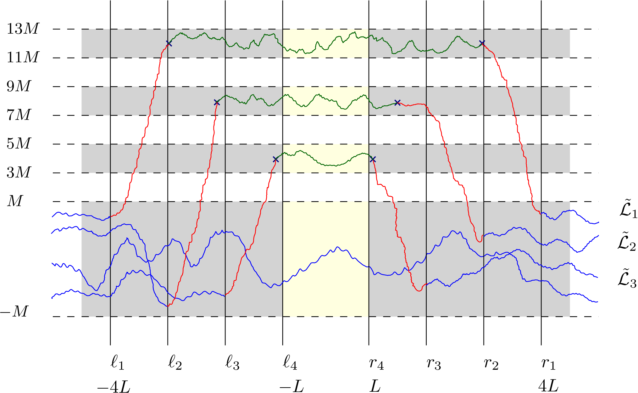
Refer to caption
Figure 5. Illustration for bounding Z𝐇t1,3,(−L,L),x→,y→,+∞,f4Z^{1,3,(-L,L),\vec{x},\vec{y},+\infty,f_{4}}_{\mathbf{H}_{t}} using two-step resampling. The blue trajectories serve as MM-Good boundary data for resampling ℒ1t,ℒ2t,ℒ3t\mathcal{L}_{1}^{t},\mathcal{L}_{2}^{t},\mathcal{L}_{3}^{t}. We hope they stay in the preferable yellow region over [−L,L][-L,L]. In that case, curves ℒ1t,ℒ2t,ℒ3t.\mathcal{L}_{1}^{t},\mathcal{L}_{2}^{t},\mathcal{L}_{3}^{t}. are separated away from each other by a distance of 2​M2M. We will do a two-step Gibbsian resampling to show that such configurations happen with a positive (uniform in tt) probability. The red trajectories are sampled in step one to have them rise up and green trajectories are sampled in step two to have them stay in the yellow region. See details of these two steps respectively in Lemma 4.4 and Lemma 4.5.

We begin with setting some parameters. Fix k∈ℕk\in\mathbb{N}, L≥1L\geq 1, t≥1t\geq 1 and take

(4.1) M≥L1/2.M\geq L^{1/2}.

For 1≤j≤k+11\leq j\leq k+1, let

ℓj≔−(k+2−j)​L,rj≔(k+2−j)​L.\displaystyle\ell_{j}\coloneqq-(k+2-j)L,\ r_{j}\coloneqq(k+2-j)L.

Consider continuous functions f=(f1,f2,…,fk)f=(f_{1},f_{2},\dots,f_{k}) with fj∈C⁡([ℓ1,ℓj]∪[rj,r1],ℝ)f_{j}\in C([\ell_{1},\ell_{j}]\cup[r_{j},r_{1}],\mathbb{R}) for 1≤j≤k1\leq j\leq k and fk+1∈C⁡([ℓ1,r1],ℝ)f_{k+1}\in C\left([\ell_{1},r_{1}],\mathbb{R}\right). We view ff as a boundary condition and call it MM-Good provided the absolute value of each component is bounded by MM.

We will consider line ensembles defined on ∪j=1k{j}×[ℓj,rj]{\cup_{j=1}^{k}\ \{j\}\times[\ell_{j},r_{j}]}. For any ff as above, we let 𝔛f\mathfrak{X}_{f} be the collection of functions ℒ=(ℒ1,ℒ2,…,ℒk)\mathcal{L}=(\mathcal{L}_{1},\mathcal{L}_{2},\dots,\mathcal{L}_{k}) with ℒj∈C⁡([ℓj,rj],ℝ)\mathcal{L}_{j}\in C([\ell_{j},r_{j}],\mathbb{R}), ℒj​(ℓj)=f⁡(ℓj)\mathcal{L}_{j}(\ell_{j})=f(\ell_{j}) and ℒj​(rj)=f⁡(rj)\mathcal{L}_{j}(r_{j})=f(r_{j}). Given ℒ∈𝔛f\mathcal{L}\in\mathfrak{X}_{f}, we may extend the domain of ℒ\mathcal{L} using ff.

ℒj,f​(u)≔{ℒj​(u)u∈[ℓj,rj],fj​(u)u∈[ℓ1,ℓj)∪(rj,r1].\displaystyle\mathcal{L}_{j,f}(u)\coloneqq\left\{\begin{array}[]{cc}\mathcal{L}_{j}(u)&u\in[\ell_{j},r_{j}],\\ f_{j}(u)&u\in[\ell_{1},\ell_{j})\cup(r_{j},r_{1}].\end{array}\right.

Note that ℒf∈C⁡([1,k]ℤ×[ℓ1,r1],ℝ)\mathcal{L}_{f}\in C([1,k]_{\mathbb{Z}}\times[\ell_{1},r_{1}],\mathbb{R}).
For j∈[1,k]ℤj\in[1,k]_{\mathbb{Z}}, let BjB_{j} be independent Brownian bridges defined on [ℓj,rj][\ell_{j},r_{j}] with Bj​(ℓj)=fj​(ℓj)B_{j}(\ell_{j})=f_{j}(\ell_{j}) and Bj​(rj)=fj​(rj)B_{j}(r_{j})=f_{j}(r_{j}). The law of BjB_{j} is given by ℙfreej,j,(ℓj,rj),fj​(ℓj),fj​(rj)\mathbb{P}_{\textup{free}}^{j,j,(\ell_{j},r_{j}),f_{j}(\ell_{j}),f_{j}(r_{j})} and we denote by ℙfree\mathbb{P}_{\textup{free}} the joint law of (B1,B2​…,Bk)(B_{1},B_{2}\dots,B_{k}) and by 𝔼free\mathbb{E}_{\textup{free}} the expectation of ℙfree\mathbb{P}_{\textup{free}}. We may view ℙfree\mathbb{P}_{\textup{free}} as a probability measure defined on 𝔛f\mathfrak{X}_{f}.

Next, we define two probability measures, ℙ\mathbb{P} and ℙ~\tilde{\mathbb{P}}, on 𝔛f\mathfrak{X}_{f} through specifying their Radon-Nikodym derivatives with respect to ℙfree\mathbb{P}_{\textup{free}}.

(4.4) d​ℙd​ℙfree​(ℒ):=1Z​W𝐇t1,k,(ℓ1,r1),x→,y→,+∞,fk+1​(ℒf),\displaystyle\frac{\textup{d}\mathbb{P}}{\textup{d}\mathbb{P}_{\textup{free}}}(\mathcal{L}):=\frac{1}{Z}W^{1,k,(\ell_{1},r_{1}),\vec{x},\vec{y},+\infty,f_{k+1}}_{\mathbf{H}_{t}}(\mathcal{L}_{f}),
(4.5) d​ℙ~d​ℙfree​(ℒ):=1Z~​W𝐇t,(−L,L)1,k,(ℓ1,r1),x→,y→,+∞,fk+1​(ℒf),\displaystyle\frac{\textup{d}\tilde{\mathbb{P}}}{\textup{d}\mathbb{P}_{\textup{free}}}(\mathcal{L}):=\frac{1}{\tilde{Z}}W^{1,k,(\ell_{1},r_{1}),\vec{x},\vec{y},+\infty,f_{k+1}}_{\mathbf{H}_{t},(-L,L)}(\mathcal{L}_{f}),

where

Z≔𝔼free​[W𝐇t1,k,(ℓ1,r1),x→,y→,+∞,fk+1​(ℒf)],\displaystyle Z\coloneqq\mathbb{E}_{\textup{free}}\left[W^{1,k,(\ell_{1},r_{1}),\vec{x},\vec{y},+\infty,f_{k+1}}_{\mathbf{H}_{t}}(\mathcal{L}_{f})\right],
Z~≔𝔼free​[W𝐇t,(−L,L)1,k,(ℓ1,r1),x→,y→,+∞,fk+1​(ℒf)],\displaystyle\tilde{Z}\coloneqq\mathbb{E}_{\textup{free}}\left[W^{1,k,(\ell_{1},r_{1}),\vec{x},\vec{y},+\infty,f_{k+1}}_{\mathbf{H}_{t},(-L,L)}(\mathcal{L}_{f})\right],

and x→=(fj​(ℓ1))j=1k\vec{x}=(f_{j}(\ell_{1}))_{j=1}^{k}, y→=(fj​(r1))j=1k\vec{y}=(f_{j}(r_{1}))_{j=1}^{k}. See Definition 2.3 for the definition of the Boltzmann weights. We denote by 𝔼\mathbb{E} and 𝔼~\tilde{\mathbb{E}} the expectation of ℙ\mathbb{P} and ℙ~\tilde{\mathbb{P}} respectively.

Consider the event that curves are well separated by order MM at the endpoints of interval [−L,L][-L,L].

𝖤:={ℒj(±L)∈[(4k−4j+3)M,(4k−4j+5)M]for allj∈[1,k]ℤ}.\displaystyle\mathsf{E}:=\left\{{\mathcal{L}}_{j}(\pm L)\in\big[(4k-4j+3)M,(4k-4j+5)M\big]\ \textup{for all}\ j\in[1,k]_{\mathbb{Z}}\right\}.

Proposition 4.1 below provides a lower bound of ℙ~​(𝖤)\tilde{\mathbb{P}}(\mathsf{E}).

Proposition 4.1.

Fix k∈ℕk\in\mathbb{N}, L≥1L\geq 1, t≥1t\geq 1 and M≥L1/2M\geq L^{1/2}. Let ff be a MM-Good boundary condition and ℙ~\tilde{\mathbb{P}} be the probability measure on 𝔛f\mathfrak{X}_{f} defined in (4.5). Then there exists a constant D3=D3​(k)D_{3}=D_{3}(k) depending only on kk such that

ℙ~​(𝖤)≥D3−1​e−D3​(L−1​M2+L).\displaystyle\tilde{\mathbb{P}}(\mathsf{E})\geq D_{3}^{-1}e^{-D_{3}(L^{-1}M^{2}+L)}.

We postpone the proof of Proposition 4.1 to the end of this section. Next, we prove a lower bound for the the normalizing constant under the law of ℙ~\tilde{\mathbb{P}} (Corollary 4.2) and under the law of ℙ\mathbb{P} (Proposition 4.3) respectively.

Corollary 4.2.

Fix k∈ℕk\in\mathbb{N}, L≥1L\geq 1, t≥1t\geq 1 and M≥L1/2M\geq L^{1/2}. Let ff be a MM-Good boundary condition and ℙ~\tilde{\mathbb{P}} be the probability measure on 𝔛f\mathfrak{X}_{f} defined in (4.5). Then there exists a constant D4=D4​(k)D_{4}=D_{4}(k) depending only on kk such that

ℙ~​(Z𝐇t1,k,(−L,L),x→,y→,+∞,fk+1≥D4−1​e−2​k​L)≥D4−1​e−D4​(L−1​M2+L).\displaystyle\tilde{\mathbb{P}}\left(Z^{1,k,(-L,L),\vec{x},\vec{y},+\infty,f_{k+1}}_{\mathbf{H}_{t}}\geq D_{4}^{-1}e^{-2kL}\right)\geq D_{4}^{-1}e^{-D_{4}(L^{-1}M^{2}+L)}.

Here x→=(ℒj​(−L))j=1k\vec{x}=({\mathcal{L}}_{j}(-L))_{j=1}^{k}, y→=(ℒj​(L))j=1k\vec{y}=({\mathcal{L}}_{j}(L))_{j=1}^{k}.

Proof.

Note that

2−1​L−1​((u+L)​ℒj​(L)+(L−u)​ℒj​(−L))2^{-1}L^{-1}\left((u+L){\mathcal{L}}_{j}(L)+(L-u){\mathcal{L}}_{j}(-L)\right)

is the interpolation function connecting (−L,ℒj​(−L))\left(-L,{\mathcal{L}}_{j}(-L)\right) and (L,ℒj​(L))\left(L,{\mathcal{L}}_{j}(L)\right). Consider the following event 𝖮𝗌𝖼\mathsf{Osc} where every layer ℒj,j=1,2,⋯,k{\mathcal{L}}_{j},j=1,2,\cdots,k does not deviate from the linear interpolation by MM,

𝖮𝗌𝖼≔{sup1≤j≤ksupu∈[−L,L]|ℒj(u)−2−1L−1((u+L)ℒj(L)+(L−u)ℒj(−L))|≤M}.\displaystyle\mathsf{Osc}\coloneqq\left\{\sup_{1\leq j\leq k}\sup_{u\in[-L,L]}\left|\mathcal{L}_{j}(u)-2^{-1}L^{-1}\left((u+L){\mathcal{L}}_{j}(L)+(L-u){\mathcal{L}}_{j}(-L)\right)\right|\leq M\right\}.

Recall that event 𝖤\mathsf{E} says that the boundary values, i.e. x→\vec{x} and y→\vec{y} are separated by at least 2​M2M. Suppose 𝖤\mathsf{E} and 𝖮𝗌𝖼\mathsf{Osc} both occur, then (ℒ1,ℒ2,…,ℒk,fk+1)({\mathcal{L}}_{1},{\mathcal{L}}_{2},\dots,{\mathcal{L}}_{k},f_{k+1}) remains ordered on [−L,L][-L,L]. In particular, the Boltzmann weight is bounded below,

(4.6) W𝐇t1,k,(−L,L),x→,y→,+∞,fk+1​(ℒ)⋅𝟙𝖤⋅𝟙𝖮𝗌𝖼≥e−2​k​L⋅𝟙𝖤⋅𝟙𝖮𝗌𝖼.W_{\mathbf{H}_{t}}^{1,k,(-L,L),\vec{x},\vec{y},+\infty,f_{k+1}}({\mathcal{L}})\cdot\mathbbm{1}_{\mathsf{E}}\cdot\mathbbm{1}_{\mathsf{Osc}}\geq e^{-2kL}\cdot\mathbbm{1}_{\mathsf{E}}\cdot\mathbbm{1}_{\mathsf{Osc}}.

Because M≥L1/2M\geq L^{1/2}, there exists D=D⁡(k)D=D(k) such that

(4.7) ℙfree1,k,(−L,L),x→,y→​(𝖮𝗌𝖼)=∏j=1kℙfreej,j,(−L,L),0,0​(supu∈[−L,L]|ℒ⁡(u)|≤M)≥D−1.\displaystyle\mathbb{P}_{\textup{free}}^{1,k,(-L,L),\vec{x},\vec{y}}(\mathsf{Osc})=\prod_{j=1}^{k}\mathbb{P}_{\textup{free}}^{j,j,(-L,L),0,0}\left(\sup_{u\in[-L,L]}|\mathcal{L}(u)|\leq M\right)\geq D^{-1}.

Recall that in (2.3),

Z𝐇t1,k,(−L,L),x→,y→,+∞,fk+1:=𝔼free1,k,(−L,L),x→,y→​[W𝐇t1,k,(−L,L),x→,y→,+∞,fk+1].\displaystyle Z_{\mathbf{H}_{t}}^{1,k,(-L,L),\vec{x},\vec{y},+\infty,f_{k+1}}:=\mathbb{E}_{\textup{free}}^{1,k,(-L,L),\vec{x},\vec{y}}\left[W_{\mathbf{H}_{t}}^{1,k,(-L,L),\vec{x},\vec{y},+\infty,f_{k+1}}\right].

Combining (2.3), (4.6) and (4.7), we get

Z𝐇t1,k,(−L,L),x→,y→,+∞,fk+1⋅𝟙𝖤≥D−1​e−2​k​L⋅𝟙𝖤.\displaystyle Z_{\mathbf{H}_{t}}^{1,k,(-L,L),\vec{x},\vec{y},+\infty,f_{k+1}}\cdot\mathbbm{1}_{\mathsf{E}}\geq D^{-1}e^{-2kL}\cdot\mathbbm{1}_{\mathsf{E}}.

This implies that 𝖤⊂{Z𝐇t1,k,(−L,L),x→,y→,+∞,fk+1≥D−1e−2​k​L}\mathsf{E}\subset\left\{Z^{1,k,(-L,L),\vec{x},\vec{y},+\infty,f_{k+1}}_{\mathbf{H}_{t}}\geq D^{-1}e^{-2kL}\right\} and the desired result then follows from Proposition 4.1. ∎

Proposition 4.3.

Fix k∈ℕk\in\mathbb{N}, L≥1L\geq 1, t≥1t\geq 1 and M≥L1/2M\geq L^{1/2}. Let ff be a MM-Good boundary condition and ℙ\mathbb{P} be the probability measure on 𝔛f\mathfrak{X}_{f} defined in (4.4). Then there exists a constant D5=D5​(k)D_{5}=D_{5}(k) depending only on kk such that for all ε∈(0,1]\varepsilon\in(0,1], we have

ℙ⁡(Z𝐇t1,k,(−L,L),x→,y→,+∞,fk+1≤ε​D5−1​e−D5​(L−1​M2+L))≤ε.\mathbb{P}\left(Z^{1,k,(-L,L),\vec{x},\vec{y},+\infty,f_{k+1}}_{\mathbf{H}_{t}}\leq\varepsilon D_{5}^{-1}e^{-D_{5}(L^{-1}M^{2}+L)}\right)\leq\varepsilon.

Here x→=(ℒj​(−L))j=1k\vec{x}=({\mathcal{L}}_{j}(-L))_{j=1}^{k}, y→=(ℒj​(L))j=1k\vec{y}=({\mathcal{L}}_{j}(L))_{j=1}^{k}.

Proof.

Let ℙ~\tilde{\mathbb{P}} be the probability measure on 𝔛f\mathfrak{X}_{f} defined in (4.5). From (4.4) and (4.5), we have

(4.8) d​ℙd​ℙ~​(ℒ)∝W𝐇t1,k,(−L,L),x→,y→,+∞,fk+1​(ℒ|[1,k]ℤ×[−L,L]),\displaystyle\frac{\textup{d}\mathbb{P}}{\textup{d}\tilde{\mathbb{P}}}(\mathcal{L})\propto W^{1,k,(-L,L),\vec{x},\vec{y},+\infty,f_{k+1}}_{\mathbf{H}_{t}}(\mathcal{L}|_{[1,k]_{\mathbb{Z}}\times[-L,L]}),

where x→=(ℒj​(−L))j=1k\vec{x}=(\mathcal{L}_{j}(-L))_{j=1}^{k} and y→=(ℒj​(L))j=1k\vec{y}=(\mathcal{L}_{j}(L))_{j=1}^{k}.

let 𝔛′\mathfrak{X}^{\prime} be the collection of functions ℒ′=(ℒ1′,ℒ2′,…,ℒk′)\mathcal{L}^{\prime}=(\mathcal{L}^{\prime}_{1},\mathcal{L}^{\prime}_{2},\dots,\mathcal{L}^{\prime}_{k}) with ℒj∈C⁡([ℓj,ℓ1]∪[r1,rj],ℝ)\mathcal{L}_{j}\in C([\ell_{j},\ell_{1}]\cup[r_{1},r_{j}],\mathbb{R}). Notice that there is the restriction map form 𝔛f\mathfrak{X}_{f} to 𝔛′\mathfrak{X}^{\prime}. Let ℙ′\mathbb{P}^{\prime} and ℙ~′\tilde{\mathbb{P}}^{\prime} be the push-forward probability measure of ℙ\mathbb{P} and ℙ~\tilde{\mathbb{P}} on 𝔛′\mathfrak{X}^{\prime} respectively. We write 𝔼′\mathbb{E}^{\prime} and 𝔼~′\tilde{\mathbb{E}}^{\prime} for the expectations for ℙ′\mathbb{P}^{\prime} and ℙ~′\tilde{\mathbb{P}}^{\prime} respectively. From (4.8), we have

d​ℙ′d​ℙ~′​(ℒ′)=1Z′​Z𝐇t1,k,(−L,L),x→,y→,+∞,fk+1.\frac{\textup{d}\mathbb{P}^{\prime}}{\textup{d}\tilde{\mathbb{P}}^{\prime}}(\mathcal{L}^{\prime})=\frac{1}{Z^{\prime}}Z_{\mathbf{H}_{t}}^{1,k,(-L,L),\vec{x},\vec{y},+\infty,f_{k+1}}.

Here x→=(ℒj′​(−L))j=1k\vec{x}=(\mathcal{L}^{\prime}_{j}(-L))_{j=1}^{k}, y→=(ℒj′​(L))j=1k\vec{y}=(\mathcal{L}^{\prime}_{j}(L))_{j=1}^{k} and Z′Z^{\prime} is a normalizing constant,

Z′=𝔼~′​[Z𝐇t1,k,(−L,L),x→,y→,+∞,fk+1].Z^{\prime}=\tilde{\mathbb{E}}^{\prime}\left[Z^{1,k,(-L,L),\vec{x},\vec{y},+\infty,f_{k+1}}_{\mathbf{H}_{t}}\right].

From Corollary 4.2,

Z′=𝔼~​[Z𝐇t1,k,(−L,L),x→,y→,+∞,fk+1]≥D4−2​e−D4​(L−1​M2+L)−2​k​L=:δ.Z^{\prime}=\tilde{\mathbb{E}}\left[Z^{1,k,(-L,L),\vec{x},\vec{y},+\infty,f_{k+1}}_{\mathbf{H}_{t}}\right]\geq D_{4}^{-2}e^{-D_{4}(L^{-1}M^{2}+L)-2kL}=:\delta.

Thus

ℙ⁡(Z𝐇t1,k,(−L,L),x→,y→,+∞,fk+1≤ε​δ)\displaystyle\mathbb{P}\left(Z^{1,k,(-L,L),\vec{x},\vec{y},+\infty,f_{k+1}}_{\mathbf{H}_{t}}\leq\varepsilon\delta\right) =ℙ′​(Z𝐇t1,k,(−L,L),x→,y→,+∞,fk+1≤ε​δ)\displaystyle=\mathbb{P}^{\prime}\left(Z^{1,k,(-L,L),\vec{x},\vec{y},+\infty,f_{k+1}}_{\mathbf{H}_{t}}\leq\varepsilon\delta\right)
=𝔼~′[1Z′Z𝐇t1,k,(−L,L),x→,y→,+∞,fk+1⋅𝟙{Z𝐇t1,k,(−L,L),x→,y→,+∞,fk+1≤εδ}]\displaystyle=\tilde{\mathbb{E}}^{\prime}\left[\frac{1}{Z^{\prime}}Z_{\mathbf{H}_{t}}^{1,k,(-L,L),\vec{x},\vec{y},+\infty,f_{k+1}}\cdot\mathbbm{1}\left\{Z^{1,k,(-L,L),\vec{x},\vec{y},+\infty,f_{k+1}}_{\mathbf{H}_{t}}\leq\varepsilon\delta\right\}\right]
≤ε​δZ′⋅𝔼~′[𝟙{Z𝐇t1,k,(−L,L),x→,y→,+∞,fk+1≤εδ}]≤ε.\displaystyle\leq\ \frac{\varepsilon\delta}{Z^{\prime}}\cdot\tilde{\mathbb{E}}^{\prime}\left[\mathbbm{1}\left\{Z^{1,k,(-L,L),\vec{x},\vec{y},+\infty,f_{k+1}}_{\mathbf{H}_{t}}\leq\varepsilon\delta\right\}\right]\leq\varepsilon.

Thus the assertion follows by picking D5​(k)=max⁡{D42,D4+2​k}D_{5}(k)=\max\{D^{2}_{4},D_{4}+2k\}. ∎

Now we are ready to prove Proposition 3.1.

Proof of Proposition 3.1.

Fix K≥L2K\geq L^{2} and let M>0M>0 be a large number to be determined soon. Throughout this proof, we write ℙℌt\mathbb{P}_{\mathfrak{H}^{t}} for the law of the scaled KPZ line ensemble. Let 𝖦𝗈𝗈𝖽𝖡𝗈𝗎𝗇𝖽𝖺𝗋𝗒\mathsf{GoodBoundary} (shorthanded as 𝖦𝖡\mathsf{GB}) be the the event that the MM-Good boundary conditions holds, i.e.

𝖦𝗈𝗈𝖽𝖡𝗈𝗎𝗇𝖽𝖺𝗋𝗒:={supu∈[ℓ1,r1]|ℌk+1t(u)|≤M}∩⋂j=1k{supu∈[ℓ1,ℓj]∪[rj,r1]|ℌjt(u)|≤M}.\displaystyle\mathsf{GoodBoundary}:=\left\{\sup_{u\in[\ell_{1},r_{1}]}|\mathfrak{H}^{t}_{k+1}(u)|\leq M\right\}\cap\bigcap_{j=1}^{k}\left\{\sup_{u\in[\ell_{1},\ell_{j}]\cup[r_{j},r_{1}]}|\mathfrak{H}^{t}_{j}(u)|\leq M\right\}.

From Corollary B.3 , by taking M=D′​KM=D^{\prime}K with suitably large D′≥1D^{\prime}\geq 1, we have

ℙℌt​(𝖦𝗈𝗈𝖽𝖡𝗈𝗎𝗇𝖽𝖺𝗋𝗒c)≤2−1​e−K3/2.\mathbb{P}_{\mathfrak{H}^{t}}(\mathsf{GoodBoundary}^{\textup{c}})\leq 2^{-1}e^{-K^{3/2}}.

Moreover, (4.1) holds. Let ℱe​x​t∗\mathcal{F}^{*}_{{ext}} be the sigma-field generated by ℌt\mathfrak{H}^{t} restricted on

ℕ×ℝ∖⋃j=1k{j}×(ℓj,rj).\displaystyle\mathbb{N}\times\mathbb{R}\setminus\bigcup_{j=1}^{k}\{j\}\times(\ell_{j},r_{j}).

By the Gibbs Property (see Definition 2.4 and Corollary 2.7),

𝔼ℌt[𝟙{Z𝐇t1,k,(−L,L),x→,y→,+∞,ℌk+1t≤2−1εD5−1e−D5​(L−1​M2+L)}|ℱe​x​t∗]\displaystyle\mathbb{E}_{\mathfrak{H}^{t}}\left[\mathbbm{1}\{Z^{1,k,(-L,L),\vec{x},\vec{y},+\infty,\mathfrak{H}^{t}_{k+1}}_{\mathbf{H}_{t}}\leq 2^{-1}\varepsilon D_{5}^{-1}e^{-D_{5}(L^{-1}M^{2}+L)}\}\,|\,\mathcal{F}^{*}_{{ext}}\right]

with x→=(ℌjt​(−L))j=1k\vec{x}=(\mathfrak{H}^{t}_{j}(-L))_{j=1}^{k} and y→=(ℌjt​(L))j=1k\vec{y}=(\mathfrak{H}^{t}_{j}(L))_{j=1}^{k} equals

ℙ⁡(Z𝐇t1,k,(−L,L),x→,y→,+∞,fk+1≤2−1​ε​D5−1​e−D5​(L−1​M2+L)),\displaystyle\mathbb{P}\left(Z^{1,k,(-L,L),\vec{x},\vec{y},+\infty,f_{k+1}}_{\mathbf{H}_{t}}\leq 2^{-1}\varepsilon D_{5}^{-1}e^{-D_{5}(L^{-1}M^{2}+L)}\right),

where ℙ\mathbb{P} is defined in (4.4) with fj=ℌjtf_{j}=\mathfrak{H}^{t}_{j} in [ℓ1,ℓj]∪[rj,r1],j∈[1,k]ℤ[\ell_{1},\ell_{j}]\cup[r_{j},r_{1}],\ j\in[1,k]_{\mathbb{Z}} and fk+1=ℌk+1tf_{k+1}=\mathfrak{H}^{t}_{k+1} in [ℓ1,r1][\ell_{1},r_{1}].

Applying Proposition 4.3 with ε=2−1​e−K3/2\varepsilon=2^{-1}e^{-K^{3/2}}, we deduce that

𝟙𝖦𝖡⋅𝔼ℌt[𝟙{Z𝐇t1,k,(ℓ,r),x→,y→,+∞,fk+1≤2−1εD5−1e−D5​(L−1​M2+L)}|ℱe​x​t∗]≤2−1e−K3/2⋅𝟙𝖦𝖡.\displaystyle\mathbbm{1}_{\mathsf{GB}}\cdot\mathbb{E}_{\mathfrak{H}^{t}}\left[\mathbbm{1}\{Z^{1,k,(\ell,r),\vec{x},\vec{y},+\infty,f_{k+1}}_{\mathbf{H}_{t}}\leq 2^{-1}\varepsilon D_{5}^{-1}e^{-D_{5}(L^{-1}M^{2}+L)}\}\,|\,\mathcal{F}^{*}_{{ext}}\right]\leq 2^{-1}e^{-K^{3/2}}\cdot\mathbbm{1}_{\mathsf{GB}}.

Thus we have

ℙℌt​(Z𝐇t1,k,(−L,L),x→,y→,+∞,fk+1≤2−1​ε​D5−1​e−D5​(L−1​M2+L))\displaystyle\mathbb{P}_{\mathfrak{H}^{t}}\left(Z^{1,k,(-L,L),\vec{x},\vec{y},+\infty,f_{k+1}}_{\mathbf{H}_{t}}\leq 2^{-1}\varepsilon D_{5}^{-1}e^{-D_{5}(L^{-1}M^{2}+L)}\right)
=\displaystyle= 𝔼ℌt[𝟙𝖦𝖡⋅𝟙{Z𝐇t1,k,(−L,L),x→,y→,+∞,fk+1≤2−1D5−1e−K3/2−D5​(L−1​M2+L)}]+ℙℌt(𝖦𝖡c)\displaystyle\mathbb{E}_{\mathfrak{H}^{t}}\left[\mathbbm{1}_{\mathsf{GB}}\cdot\mathbbm{1}\left\{Z^{1,k,(-L,L),\vec{x},\vec{y},+\infty,f_{k+1}}_{\mathbf{H}_{t}}\leq 2^{-1}D_{5}^{-1}e^{-K^{3/2}-D_{5}(L^{-1}M^{2}+L)}\right\}\right]+\mathbb{P}_{\mathfrak{H}^{t}}(\mathsf{GB}^{\textup{c}})
≤\displaystyle\leq e−K3/2.\displaystyle e^{-K^{3/2}}.

Because K≥L2K\geq L^{2} and M=D′​KM=D^{\prime}K, we have 2−1​D5−1​e−K3/2−D5​(L−1​M2+L)≥D−1​e−D​L−1​K22^{-1}D_{5}^{-1}e^{-K^{3/2}-D_{5}(L^{-1}M^{2}+L)}\geq D^{-1}e^{-DL^{-1}K^{2}}. The proof is finished. ∎

The rest of this section is devoted to proving Proposition 4.1. We will run a two-step inductive resampling. For j∈[1,k]ℤj\in[1,k]_{\mathbb{Z}}, consider a sequence of events

(4.9) 𝖠j:={infu∈[ℓj+1,rj+1]ℒj(u)≥(4k−4j+4)M}.\displaystyle\mathsf{A}_{j}:=\bigg\{\inf_{u\in[\ell_{j+1},r_{j+1}]}{\mathcal{L}}_{j}(u)\geq(4k-4j+4)M\bigg\}.

The first step is carried out inductively in Lemma 4.4 to raise curves and hence give a lower bound of ℙ~​(⋂j=1k𝖠j)\tilde{\mathbb{P}}\bigg(\bigcap_{j=1}^{k}\mathsf{A}_{j}\bigg). Denote

(4.10) 𝖥j:=\displaystyle\mathsf{F}_{j}:= {ℒj∈[(4k−4j+3)M,(4k−4j+5)M]in[ℓj+1,rj+1]}\displaystyle\bigg\{{\mathcal{L}}_{j}\in[(4k-4j+3)M,(4k-4j+5)M]\ \textup{in}\ [\ell_{j+1},r_{j+1}]\bigg\}
∩{ℒj≤(4k−4j+5)Min[ℓj,rj]}.\displaystyle\cap\bigg\{{\mathcal{L}}_{j}\leq(4k-4j+5)M\ \textup{in}\ [\ell_{j},r_{j}]\bigg\}.

The second step is carried out inductively to lower curve properly in order to separate them in the desired region. See Lemma 4.5, which gives a lower bound of ℙ~​(⋂j=1k𝖥j)\tilde{\mathbb{P}}\bigg(\bigcap_{j=1}^{k}\mathsf{F}_{j}\bigg). Proposition 4.1 follows directly from the Lemma 4.5 as ⋂j=1k𝖥j⊂𝖤\displaystyle\bigcap_{j=1}^{k}\mathsf{F}_{j}\subset\mathsf{E}.

Lemma 4.4.

Fix k∈ℕk\in\mathbb{N}, L≥1L\geq 1, t≥1t\geq 1 and M≥L1/2M\geq L^{1/2}. Let ff be a MM-Good boundary condition and ℙ~\tilde{\mathbb{P}} be the probability measure on 𝔛f\mathfrak{X}_{f} defined in (4.5). Then there exists a constant D6=D6​(k)D_{6}=D_{6}(k) depending only on kk such that

ℙ~​(⋂j=1k𝖠j)≥D6−1​e−D6​(L−1​M2+L).\displaystyle\tilde{\mathbb{P}}\bigg(\bigcap_{j=1}^{k}\mathsf{A}_{j}\bigg)\geq D_{6}^{-1}e^{-D_{6}(L^{-1}M^{2}+L)}.
Refer to caption
Figure 6. A realization of ⋂j=1k𝖠j\bigcap_{j=1}^{k}\mathsf{A}_{j} with k=3k=3. This is an illustration of the step one resampling. We first resample ℒ1{\mathcal{L}}_{1} to have it rise above 12​M12M within [ℓ1,ℓ2][\ell_{1},\ell_{2}] and [r1,r2][r_{1},r_{2}] and also have it stay above 12​M12M after they reach it. Then resample ℒ2{\mathcal{L}}_{2} to have it rise above 8​M8M within [ℓ2,ℓ3][\ell_{2},\ell_{3}] and [r2,r3][r_{2},r_{3}] and also have it stay above 8​M8M after they reach it. Furthermore resample ℒ3{\mathcal{L}}_{3} to have it rise above 4​M4M within [ℓ3,ℓ4][\ell_{3},\ell_{4}] and [r3,r4][r_{3},r_{4}] and also have it stay above 4​M4M after they reach it.
Proof.

We start by showing the lower bound for ℙ~​(𝖠1)\tilde{\mathbb{P}}(\mathsf{A}_{1}). From (4.5) and the Gibbs property (see Definition 2.4),

𝔼~​[𝟙𝖠1|ℱe​x​t​({1}×(ℓ1,r1))]=ℙ𝐇t,(−L,L)1,1,(ℓ1,r1),f1​(ℓ1),f1​(r1),+∞,ℒ2,f​(𝖠1)\displaystyle\tilde{\mathbb{E}}[\mathbbm{1}_{\mathsf{A}_{1}}\,|\,\mathcal{F}_{{ext}}(\{1\}\times(\ell_{1},r_{1}))]={\mathbb{P}_{\mathbf{H}_{t},(-L,L)}^{1,1,(\ell_{1},r_{1}),f_{1}(\ell_{1}),f_{1}(r_{1}),+\infty,\mathcal{{L}}_{2,f}}({\mathsf{A}_{1}})}

with ℒ2,f\mathcal{{L}}_{2,f} defined by (4). Note that equivalently we have

ℙ𝐇t,(−L,L)1,1,(ℓ1,r1),f1​(ℓ1),f1​(r1),+∞,ℒ2,f=ℙ𝐇t1,1,(ℓ1,r1),f1​(ℓ1),f1​(r1),+∞,g2{\mathbb{P}_{\mathbf{H}_{t},(-L,L)}^{1,1,(\ell_{1},r_{1}),f_{1}(\ell_{1}),f_{1}(r_{1}),+\infty,\mathcal{{L}}_{2,f}}}={\mathbb{P}_{\mathbf{H}_{t}}^{1,1,(\ell_{1},r_{1}),f_{1}(\ell_{1}),f_{1}(r_{1}),+\infty,g_{2}}}

with

g2​(u)≔{ℒ2,f​(u)u∈[ℓ1,−L)∪(L,r1],−∞u∈[−L,L].\displaystyle g_{2}(u)\coloneqq\left\{\begin{array}[]{cc}\mathcal{{L}}_{2,f}(u)&u\in[\ell_{1},-L)\cup(L,r_{1}],\\ -\infty&u\in[-L,L].\end{array}\right.

Using the stochastic monotonicity, Lemma 2.10, we have

ℙ𝐇t1,1,(ℓ1,r1),f1​(ℓ1),f1​(r1),+∞,g2​(𝖠1)\displaystyle{\mathbb{P}_{\mathbf{H}_{t}}^{1,1,(\ell_{1},r_{1}),f_{1}(\ell_{1}),f_{1}(r_{1}),+\infty,g_{2}}({\mathsf{A}_{1}})} ≥ℙ𝐇t1,1,(ℓ1,r1),f1​(ℓ1),f1​(r1),+∞,−∞​(𝖠1)\displaystyle\geq{\mathbb{P}_{\mathbf{H}_{t}}^{1,1,(\ell_{1},r_{1}),f_{1}(\ell_{1}),f_{1}(r_{1}),+\infty,-\infty}({\mathsf{A}_{1}})}
=ℙfree1,1,(ℓ1,r1),f1​(ℓ1),f1​(r1)​(𝖠1).\displaystyle=\mathbb{P}_{\textup{free}}^{1,1,(\ell_{1},r_{1}),f_{1}(\ell_{1}),f_{1}(r_{1})}\left({\mathsf{A}_{1}}\right).

Let

a1≔inf{ℙfree1,1,(ℓ1,r1),x,y(𝖠1)||x|≤M,|y|≤M}.\displaystyle a_{1}\coloneqq\inf\left\{\mathbb{P}_{\textup{free}}^{1,1,(\ell_{1},r_{1}),x,y}\left({\mathsf{A}_{1}}\right)\,\Big|\,|x|\leq M,\ |y|\leq M\right\}.

Under MM-Good boundary conditions, M≥L1/2M\geq L^{1/2}, we seek for a lower bound of a1a_{1}. To realize 𝖠1\mathsf{A}_{1}, it suffices to have the Brownian bridge B1B_{1} first jump over a height (4​k+2)​M(4k+2)M within the interval [ℓ1,ℓ2][\ell_{1},\ell_{2}], secondly remain above 4​k​M4kM within the interval [ℓ2,r2][\ell_{2},r_{2}], and thirdly drop down a height (4​k+2)​M(4k+2)M within [r2,r1][r_{2},r_{1}]. a1a_{1} is bounded below by the Brownian kinetic cost of such trajectory. Note that |ℓ2−ℓ1|=|r2−r1|=L|\ell_{2}-\ell_{1}|=|r_{2}-r_{1}|=L and |ℓ2−r2|=2​k​L|\ell_{2}-r_{2}|=2kL. Hence there exists D=D⁡(k)D=D(k) such that a1≥D−1​e−D​L−1​M2.a_{1}\geq D^{-1}e^{-DL^{-1}M^{2}}. Thus we deduce

ℙ~​(𝖠1)\displaystyle\tilde{\mathbb{P}}(\mathsf{A}_{1}) =𝔼~​[𝔼~​[𝟙𝖠1|ℱe​x​t​({1}×(ℓ1,r1))]]\displaystyle=\tilde{\mathbb{E}}\left[\tilde{\mathbb{E}}[\mathbbm{1}_{\mathsf{A}_{1}}\,|\,\mathcal{F}_{{ext}}(\{1\}\times(\ell_{1},r_{1}))]\right]
≥ℙfree1,1,(ℓ1,r1),f1​(ℓ1),f1​(r1)​(𝖠1)≥D−1​e−D​L−1​M2.\displaystyle\geq\mathbb{P}_{\textup{free}}^{1,1,(\ell_{1},r_{1}),f_{1}(\ell_{1}),f_{1}(r_{1})}\left({\mathsf{A}_{1}}\right)\geq D^{-1}e^{-DL^{-1}M^{2}}.

Now we proceed by induction on jj. Assume for j∈[2,k]ℤj\in[2,k]_{\mathbb{Z}}, we have

ℙ~​(⋂i=1j−1𝖠i)≥D−1​e−D⁡(L−1​M2+L).\tilde{\mathbb{P}}\bigg(\bigcap_{i=1}^{j-1}\mathsf{A}_{i}\bigg)\geq D^{-1}e^{-D(L^{-1}M^{2}+L)}.

We aim to show

ℙ~​(⋂i=1j𝖠i)≥D−1​e−D⁡(L−1​M2+L).\tilde{\mathbb{P}}\bigg(\bigcap_{i=1}^{j}\mathsf{A}_{i}\bigg)\geq D^{-1}e^{-D(L^{-1}M^{2}+L)}.

From (4.5) and the Gibbs property (see Definition 2.4),

𝔼~​[𝟙𝖠j|ℱe​x​t​({j}×(ℓj,rj))]=ℙ𝐇t,(−L,L)j,j,(ℓj,rj),fj​(ℓj),fj​(rj),ℒj−1,ℒj+1,f​(𝖠j),\displaystyle\tilde{\mathbb{E}}[\mathbbm{1}_{\mathsf{A}_{j}}\,|\,\mathcal{F}_{{ext}}(\{j\}\times(\ell_{j},r_{j}))]=\mathbb{P}^{j,j,(\ell_{j},r_{j}),f_{j}(\ell_{j}),f_{j}(r_{j}),{\mathcal{L}}_{j-1},{\mathcal{L}}_{j+1,f}}_{\mathbf{H}_{t},(-L,L)}(\mathsf{A}_{j}),

with ℒj+1,f{\mathcal{L}}_{j+1,f} defined in (4) and we adopt the convention that ℒk+1,f=fk+1{\mathcal{L}}_{k+1,f}=f_{k+1}. Note that

ℙ𝐇t,(−L,L)j,j,(ℓj,rj),fj​(ℓj),fj​(rj),ℒj−1,ℒj+1,f=ℙ𝐇tj,j,(ℓj,rj),fj​(ℓj),fj​(rj),gj−1,gj+1\displaystyle\mathbb{P}^{j,j,(\ell_{j},r_{j}),f_{j}(\ell_{j}),f_{j}(r_{j}),{\mathcal{L}}_{j-1},{\mathcal{L}}_{j+1,f}}_{\mathbf{H}_{t},(-L,L)}=\mathbb{P}^{j,j,(\ell_{j},r_{j}),f_{j}(\ell_{j}),f_{j}(r_{j}),g_{j-1},g_{j+1}}_{\mathbf{H}_{t}}

with

gj−1​(u)≔{ℒj−1​(u)u∈[ℓj,−L)∪(L,rj],+∞u∈[−L,L],\displaystyle g_{j-1}(u)\coloneqq\left\{\begin{array}[]{cc}\mathcal{{L}}_{j-1}(u)&u\in[\ell_{j},-L)\cup(L,r_{j}],\\ +\infty&u\in[-L,L],\end{array}\right.

and

gj+1​(u)≔{ℒj+1,f​(u)u∈[ℓj,−L)∪(L,rj],−∞u∈[−L,L].\displaystyle g_{j+1}(u)\coloneqq\left\{\begin{array}[]{cc}\mathcal{{L}}_{j+1,f}(u)&u\in[\ell_{j},-L)\cup(L,r_{j}],\\ -\infty&u\in[-L,L].\end{array}\right.

We claim that

(4.11) 𝔼~​[𝟙𝖠j|ℱe​x​t​({j}×(ℓj,rj))]≥𝔼freej,j,(ℓj,rj),fj​(ℓj),fj​(rj)​[𝟙𝖠j⋅W𝐇tj,j,(ℓj,rj),fj​(ℓj),fj​(rj),gj−1,−∞].\tilde{\mathbb{E}}[\mathbbm{1}_{\mathsf{A}_{j}}\,|\,\mathcal{F}_{{ext}}(\{j\}\times(\ell_{j},r_{j}))]\geq\mathbb{E}_{\textup{free}}^{j,j,(\ell_{j},r_{j}),f_{j}(\ell_{j}),f_{j}(r_{j})}\left[\mathbbm{1}_{\mathsf{A}_{j}}\cdot W^{j,j,(\ell_{j},r_{j}),f_{j}(\ell_{j}),f_{j}(r_{j}),g_{j-1},-\infty}_{\mathbf{H}_{t}}\right].

This can be derived as

𝔼~​[𝟙𝖠j|ℱe​x​t​({j}×(ℓj,rj))]\displaystyle\tilde{\mathbb{E}}[\mathbbm{1}_{\mathsf{A}_{j}}\,|\,\mathcal{F}_{{ext}}(\{j\}\times(\ell_{j},r_{j}))] =ℙ𝐇tj,j,(ℓj,rj),fj​(ℓj),fj​(rj),gj−1,gj+1​(𝖠j)\displaystyle=\mathbb{P}^{j,j,(\ell_{j},r_{j}),f_{j}(\ell_{j}),f_{j}(r_{j}),g_{j-1},g_{j+1}}_{\mathbf{H}_{t}}(\mathsf{A}_{j})
≥ℙ𝐇tj,j,(ℓj,rj),fj​(ℓj),fj​(rj),gj−1,−∞​(𝖠j)\displaystyle\geq\mathbb{P}^{j,j,(\ell_{j},r_{j}),f_{j}(\ell_{j}),f_{j}(r_{j}),g_{j-1},-\infty}_{\mathbf{H}_{t}}(\mathsf{A}_{j})
=1Z𝐇t​𝔼freej,j,(ℓj,rj),fj​(ℓj),fj​(rj)​[𝟙𝖠j⋅W𝐇tj,j,(ℓj,rj),fj​(ℓj),fj​(rj),gj−1,−∞].\displaystyle=\frac{1}{Z_{\mathbf{H}_{t}}}\mathbb{E}_{\textup{free}}^{j,j,(\ell_{j},r_{j}),f_{j}(\ell_{j}),f_{j}(r_{j})}\left[\mathbbm{1}_{\mathsf{A}_{j}}\cdot W^{j,j,(\ell_{j},r_{j}),f_{j}(\ell_{j}),f_{j}(r_{j}),g_{j-1},-\infty}_{\mathbf{H}_{t}}\right].
≥𝔼freej,j,(ℓj,rj),fj​(ℓj),fj​(rj)​[𝟙𝖠j⋅W𝐇tj,j,(ℓj,rj),fj​(ℓj),fj​(rj),gj−1,−∞].\displaystyle\geq\mathbb{E}_{\textup{free}}^{j,j,(\ell_{j},r_{j}),f_{j}(\ell_{j}),f_{j}(r_{j})}\left[\mathbbm{1}_{\mathsf{A}_{j}}\cdot W^{j,j,(\ell_{j},r_{j}),f_{j}(\ell_{j}),f_{j}(r_{j}),g_{j-1},-\infty}_{\mathbf{H}_{t}}\right].

Here the in the second equality we use Z𝐇tZ_{\mathbf{H}_{t}} to abbreviate

Z𝐇t:=𝔼freej,j,(ℓj,rj),fj​(ℓj),fj​(rj)​[W𝐇tj,j,(ℓj,rj),fj​(ℓj),fj​(rj),gj−1,−∞].Z_{\mathbf{H}_{t}}:=\mathbb{E}_{\textup{free}}^{j,j,(\ell_{j},r_{j}),f_{j}(\ell_{j}),f_{j}(r_{j})}\left[W^{j,j,(\ell_{j},r_{j}),f_{j}(\ell_{j}),f_{j}(r_{j}),g_{j-1},-\infty}_{\mathbf{H}_{t}}\right].

In the first inequality we apply stochastic monotonicity, Lemma 2.10, and in the second inequality we use the fact that normalizing constant is bounded from above by 1.

Now we proceed to find a lower bound for

𝟙𝖠j−1⋅𝔼freej,j,(ℓj,rj),fj​(ℓj),fj​(rj)​[𝟙𝖠j⋅W𝐇tj,j,(ℓj,rj),fj​(ℓj),fj​(rj),gj−1,−∞].\mathbbm{1}_{\mathsf{A}_{j-1}}\cdot\mathbb{E}_{\textup{free}}^{j,j,(\ell_{j},r_{j}),f_{j}(\ell_{j}),f_{j}(r_{j})}\left[\mathbbm{1}_{\mathsf{A}_{j}}\cdot W^{j,j,(\ell_{j},r_{j}),f_{j}(\ell_{j}),f_{j}(r_{j}),g_{j-1},-\infty}_{\mathbf{H}_{t}}\right].

Consider the event

𝖣j:=\displaystyle\mathsf{D}_{j}:= {infu∈[ℓj+1,rj+1]ℒj(u)≥(4k−4j+4)M}∩{supu∈[ℓj,rj]ℒj(u)≤(4k−4j+8)M}.\displaystyle\bigg\{\inf_{u\in[\ell_{j+1},r_{j+1}]}{\mathcal{L}}_{j}(u)\geq(4k-4j+4)M\bigg\}\cap\bigg\{\sup_{u\in[\ell_{j},r_{j}]}{\mathcal{L}}_{j}(u)\leq(4k-4j+8)M\bigg\}.

Note that 𝖣j⊂𝖠j\mathsf{D}_{j}\subset\mathsf{A}_{j}. As 𝖣j\mathsf{D}_{j} and 𝖠j−1\mathsf{A}_{j-1} occur, ℒj−1≥ℒj{\mathcal{L}}_{j-1}\geq{\mathcal{L}}_{j} in [ℓj,rj][\ell_{j},r_{j}] and hence

W𝐇tj,j,(ℓj,rj),fj​(ℓj),fj​(rj),gj−1,−∞⋅𝟙𝖣j⋅𝟙𝖠j−1≥e−2​(k+1−j)​L⋅𝟙𝖣j⋅𝟙𝖠j−1.\displaystyle W^{j,j,(\ell_{j},r_{j}),f_{j}(\ell_{j}),f_{j}(r_{j}),g_{j-1},-\infty}_{\mathbf{H}_{t}}\cdot\mathbbm{1}_{\mathsf{D}_{j}}\cdot\mathbbm{1}_{\mathsf{A}_{j-1}}\geq e^{-2(k+1-j)L}\cdot\mathbbm{1}_{\mathsf{D}_{j}}\cdot\mathbbm{1}_{\mathsf{A}_{j-1}}.

Consequently

𝟙𝖠j−1​𝔼freej,j,(ℓj,rj),fj​(ℓj),fj​(rj)​[𝟙𝖠j⋅W𝐇tj,j,(ℓj,rj),fj​(ℓj),fj​(rj),gj−1,−∞]≥𝟙𝖠j−1​𝔼freej,j,(ℓj,rj),fj​(ℓj),fj​(rj)​[𝟙𝖣j⋅W𝐇tj,j,(ℓj,rj),fj​(ℓj),fj​(rj),gj−1,−∞]≥𝟙𝖠j−1​𝔼freej,j,(ℓj,rj),fj​(ℓj),fj​(rj)​[𝟙𝖣j⋅e−2​(k+1−j)​L]≥𝟙𝖠j−1⋅e−2​(k+1−j)​L​ℙfreej,j,(ℓj,rj),x,y​(𝖣j).\begin{split}&\mathbbm{1}_{\mathsf{A}_{j-1}}\mathbb{E}_{\textup{free}}^{j,j,(\ell_{j},r_{j}),f_{j}(\ell_{j}),f_{j}(r_{j})}\left[\mathbbm{1}_{\mathsf{A}_{j}}\cdot W^{j,j,(\ell_{j},r_{j}),f_{j}(\ell_{j}),f_{j}(r_{j}),g_{j-1},-\infty}_{\mathbf{H}_{t}}\right]\\ &\geq\mathbbm{1}_{\mathsf{A}_{j-1}}\mathbb{E}_{\textup{free}}^{j,j,(\ell_{j},r_{j}),f_{j}(\ell_{j}),f_{j}(r_{j})}\left[\mathbbm{1}_{\mathsf{D}_{j}}\cdot W^{j,j,(\ell_{j},r_{j}),f_{j}(\ell_{j}),f_{j}(r_{j}),g_{j-1},-\infty}_{\mathbf{H}_{t}}\right]\\ &\geq\mathbbm{1}_{\mathsf{A}_{j-1}}\mathbb{E}_{\textup{free}}^{j,j,(\ell_{j},r_{j}),f_{j}(\ell_{j}),f_{j}(r_{j})}\left[\mathbbm{1}_{\mathsf{D}_{j}}\cdot e^{-2(k+1-j)L}\right]\\ &\geq\mathbbm{1}_{\mathsf{A}_{j-1}}\cdot e^{-2(k+1-j)L}\mathbb{P}_{\textup{free}}^{j,j,(\ell_{j},r_{j}),x,y}(\mathsf{D}_{j}).\end{split}

In short, we derived

(4.12) 𝟙𝖠j−1​𝔼freej,j,(ℓj,rj),fj​(ℓj),fj​(rj)​[𝟙𝖠j⋅W𝐇tj,j,(ℓj,rj),fj​(ℓj),fj​(rj),gj−1,−∞]≥𝟙𝖠j−1⋅e−2​(k+1−j)​L​ℙfreej,j,(ℓj,rj),x,y​(𝖣j).\begin{split}&\mathbbm{1}_{\mathsf{A}_{j-1}}\mathbb{E}_{\textup{free}}^{j,j,(\ell_{j},r_{j}),f_{j}(\ell_{j}),f_{j}(r_{j})}\left[\mathbbm{1}_{\mathsf{A}_{j}}\cdot W^{j,j,(\ell_{j},r_{j}),f_{j}(\ell_{j}),f_{j}(r_{j}),g_{j-1},-\infty}_{\mathbf{H}_{t}}\right]\\ \geq&\mathbbm{1}_{\mathsf{A}_{j-1}}\cdot e^{-2(k+1-j)L}\mathbb{P}_{\textup{free}}^{j,j,(\ell_{j},r_{j}),x,y}(\mathsf{D}_{j}).\end{split}

From Lemma A.4, the MM-Good boundary condition implies that there exists D=D⁡(k)D=D(k) such that

(4.13) aj\displaystyle a_{j} :=inf{ℙfreej,j,(ℓj,rj),x,y(𝖣j)||x|≤M,|y|≤M}≥D−1e−D​L−1​M2.\displaystyle:=\inf\left\{\mathbb{P}_{\textup{free}}^{j,j,(\ell_{j},r_{j}),x,y}(\mathsf{D}_{j})\,|\,|x|\leq M,\ |y|\leq M\right\}\geq D^{-1}e^{-DL^{-1}M^{2}}.

From (4.11), (4.12), (4.13) and the induction hypothesis, we have

ℙ~​(⋂i=1j𝖠i)=\displaystyle\tilde{\mathbb{P}}\bigg(\bigcap_{i=1}^{j}\mathsf{A}_{i}\bigg)= 𝔼~​[∏i=1j−1𝟙𝖠i⋅𝔼~​[𝟙𝖠j|ℱe​x​t​({j}×(ℓj,rj))]]\displaystyle\tilde{\mathbb{E}}\left[\prod_{i=1}^{j-1}\mathbbm{1}_{\mathsf{A}_{i}}\cdot\tilde{\mathbb{E}}[\mathbbm{1}_{\mathsf{A}_{j}}\,|\,\mathcal{F}_{{ext}}(\{j\}\times(\ell_{j},r_{j}))]\right]
≥aj⋅e−2​(k+1−j)​L⋅ℙ~​(⋂i=1j−1𝖠i)\displaystyle\geq a_{j}\cdot e^{-2(k+1-j)L}\cdot\tilde{\mathbb{P}}\bigg(\bigcap_{i=1}^{j-1}\mathsf{A}_{i}\bigg)
≥D−1​e−D⁡(L−1​M2+L).\displaystyle\geq D^{-1}e^{-D(L^{-1}M^{2}+L)}.

This completes the induction argument and hence proves the desired result. ∎

For j∈[1,k]ℤj\in[1,k]_{\mathbb{Z}}, recall the events

𝖥j:=\displaystyle\mathsf{F}_{j}:= {ℒj∈[(4k−4j+3)M,(4k−4j+5)M]in[ℓj+1,rj+1]}\displaystyle\bigg\{{\mathcal{L}}_{j}\in[(4k-4j+3)M,(4k-4j+5)M]\ \textup{in}\ [\ell_{j+1},r_{j+1}]\bigg\}
∩{ℒj≤(4k−4j+5)Min[ℓj,rj]}.\displaystyle\cap\bigg\{{\mathcal{L}}_{j}\leq(4k-4j+5)M\ \textup{in}\ [\ell_{j},r_{j}]\bigg\}.

In the following Lemma 4.5, we give a lower bound for ℙ~​(⋂j=1k𝖥j)\tilde{\mathbb{P}}\bigg(\bigcap_{j=1}^{k}\mathsf{F}_{j}\bigg).

Lemma 4.5.

Fix k∈ℕk\in\mathbb{N}, L≥1L\geq 1, t≥1t\geq 1 and M≥L1/2M\geq L^{1/2}. Let ff be a MM-Good boundary condition and ℙ~\tilde{\mathbb{P}} be the probability measure on 𝔛f\mathfrak{X}_{f} defined in (4.5). Then there exists a constant D7=D7​(k)D_{7}=D_{7}(k) such that

ℙ~​(⋂j=1k𝖥j)≥D7−1​e−D7​(L−1​M2+L).\displaystyle\tilde{\mathbb{P}}\bigg(\bigcap_{j=1}^{k}\mathsf{F}_{j}\bigg)\geq D_{7}^{-1}e^{-D_{7}(L^{-1}M^{2}+L)}.
Refer to caption
Figure 7. A realization of ⋂j=1k𝖥j\bigcap_{j=1}^{k}\mathsf{F}_{j} with k=3k=3. This is an illustration of the step two resampling. First for ℒ3{\mathcal{L}}_{3}, find the {3}\{3\}-stopping domain (𝔩3,𝔯3)(\mathfrak{l}_{3},\mathfrak{r}_{3}) where it first hits 4​M4M from left and right respectively. Then resample ℒ3{\mathcal{L}}_{3} on [𝔩3,𝔯3][\mathfrak{l}_{3},\mathfrak{r}_{3}] to have it stay within [3​M,5​M][3M,5M]. Then for ℒ2{\mathcal{L}}_{2}, find the {2}\{2\}-stopping domain (𝔩2,𝔯2)(\mathfrak{l}_{2},\mathfrak{r}_{2}) where it first hits 8​M8M from left and right respectively. Then resample ℒ2{\mathcal{L}}_{2} on [𝔩2,𝔯2][\mathfrak{l}_{2},\mathfrak{r}_{2}] to have it stay within [7​M,9​M][7M,9M]. Lastly for ℒ1{\mathcal{L}}_{1}, find the {1}\{1\}-stopping domain (𝔩1,𝔯1)(\mathfrak{l}_{1},\mathfrak{r}_{1}) where it first hits 12​M12M from left and right respectively. Then resample ℒ1{\mathcal{L}}_{1} on [𝔩1,𝔯1][\mathfrak{l}_{1},\mathfrak{r}_{1}] to have it stay within [11​M,13​M][11M,13M].
Proof.

We will run a resampling in a reversed order starting from the kk-layer and argue inductively. More precisely, we start by showing a lower bound for ℙ~​(⋂j=1k−1𝖠j∩𝖥k)\tilde{\mathbb{P}}\bigg(\bigcap_{j=1}^{k-1}\mathsf{A}_{j}\cap\mathsf{F}_{k}\bigg).

Let [𝔩k,𝔯k][\mathfrak{l}_{k},\mathfrak{r}_{k}] be a {k}\{k\}-stopping domain such that

𝔩k:=\displaystyle\mathfrak{l}_{k}:= sup{u∈[ℓk,ℓk+1]|ℒk​(u′)<4​M​for all​u′∈[ℓk,u]},\displaystyle\sup\big\{u\in[\ell_{k},\ell_{k+1}]\ |\ {\mathcal{L}}_{k}(u^{\prime})<4M\ \textup{for all}\ u^{\prime}\in[\ell_{k},u]\big\},
𝔯k:=\displaystyle\mathfrak{r}_{k}:= inf{u∈[rk+1,rk]|ℒk​(u′)<4​M​for all​u′∈[u,rk]},\displaystyle\inf\big\{u\in[r_{k+1},r_{k}]\ |\ {\mathcal{L}}_{k}(u^{\prime})<4M\ \textup{for all}\ u^{\prime}\in[u,r_{k}]\big\},

where we set 𝔩k=ℓk\mathfrak{l}_{k}=\ell_{k} or 𝔯k=rk\mathfrak{r}_{k}=r_{k} if the sets are empty respectively. Consider the event

𝖥k′:={ℒk(𝔩k)=ℒk(𝔯k)=4M}.\displaystyle\mathsf{F}^{\prime}_{k}:=\bigg\{{\mathcal{L}}_{k}(\mathfrak{l}_{k})={\mathcal{L}}_{k}(\mathfrak{r}_{k})=4M\bigg\}.

Because ℒk​(ℓk),ℒk​(rk)∈[−M,M]{\mathcal{L}}_{k}(\ell_{k}),{\mathcal{L}}_{k}(r_{k})\in[-M,M], we have 𝖠k⊂𝖥k′\mathsf{A}_{k}\subset\mathsf{F}^{\prime}_{k}. In the view of Lemma 4.4,

(4.14) ℙ~​(⋂j=1k−1𝖠j∩𝖥k′)≥D−1​e−D⁡(L−1​M2+L).\tilde{\mathbb{P}}\bigg(\bigcap_{j=1}^{k-1}\mathsf{A}_{j}\cap\mathsf{F}^{\prime}_{k}\bigg)\geq D^{-1}e^{-D(L^{-1}M^{2}+L)}.

We would like to have ℒk{\mathcal{L}}_{k} stay in the preferable region [3​M,5​M][3M,5M] over [𝔩k,𝔯k][\mathfrak{l}_{k},\mathfrak{r}_{k}]. Let

𝖥k′′≔{ℒk∈[3M,5M]in[𝔩k,𝔯k]}.\displaystyle\mathsf{F}_{k}^{\prime\prime}\coloneqq\{{\mathcal{L}}_{k}\in[3M,5M]\ \textup{in}\ [\mathfrak{l}_{k},\mathfrak{r}_{k}]\}.

Note that the occurrence of 𝖠k−1∩𝖥k′′\mathsf{A}_{k-1}\cap\mathsf{F}^{\prime\prime}_{k} implies ordering between ℒk−1{\mathcal{L}}_{k-1} and ℒk{\mathcal{L}}_{k}, i.e.

𝖠k−1∩𝖥k′′⊂{ℒk−1≥ℒk≥fk+1in[𝔩k,𝔯k]}.\displaystyle\mathsf{A}_{k-1}\cap\mathsf{F}^{\prime\prime}_{k}\subset\{{\mathcal{L}}_{k-1}\geq{\mathcal{L}}_{k}\geq f_{k+1}\ \textup{in}\ [\mathfrak{l}_{k},\mathfrak{r}_{k}]\}.

Hence

W𝐇t,(−L,L)k,k,(𝔩k,𝔯k),ℒ~k​(𝔩k),ℒ~k​(𝔯k),ℒk−1,fk+1⋅𝟙𝖠k−1⋅𝟙𝖥k′′≥e−4​L⋅𝟙𝖠k−1⋅𝟙𝖥k′′.\displaystyle W^{k,k,(\mathfrak{l}_{k},\mathfrak{r}_{k}),\mathcal{\tilde{L}}_{k}(\mathfrak{l}_{k}),\mathcal{\tilde{L}}_{k}(\mathfrak{r}_{k}),{\mathcal{L}}_{k-1},f_{k+1}}_{\mathbf{H}_{t},(-L,L)}\cdot\mathbbm{1}_{\mathsf{A}_{k-1}}\cdot\mathbbm{1}_{\mathsf{F}_{k}^{\prime\prime}}\geq e^{-4L}\cdot\mathbbm{1}_{\mathsf{A}_{k-1}}\cdot\mathbbm{1}_{\mathsf{F}_{k}^{\prime\prime}}.

And

(4.15) 1𝖠k−1⋅𝟙𝖥k′⋅𝔼~​[𝟙𝖥k′′|ℱe​x​t​({k}×(𝔩k,𝔯k))]=𝟙𝖠k−1⋅𝟙𝖥k′⋅ℙ𝐇t,(−L,L)k,k,(𝔩k,𝔯k),ℒ~k​(𝔩k),ℒ~k​(𝔯k),ℒk−1,fk+1​(𝖥k′′)≥𝟙𝖠k−1⋅𝟙𝖥k′⋅𝔼freek,k,(𝔩k,𝔯k),ℒ~k​(𝔩k),ℒ~k​(𝔯k)​[𝟙𝖥k′′⋅W𝐇t,(−L,L)k,k,(𝔩k,𝔯k),ℒ~k​(𝔩k),ℒ~k​(𝔯k),ℒk−1,fk+1]≥𝟙𝖠k−1⋅𝟙𝖥k′⋅e−4​L⋅ℙfreek,k,(𝔩k,𝔯k),4​M,4​M​(𝖥k′′).\begin{split}&\quad\ \mathbbm{1}_{\mathsf{A}_{k-1}}\cdot\mathbbm{1}_{\mathsf{F}^{\prime}_{k}}\cdot\tilde{\mathbb{E}}[\mathbbm{1}_{\mathsf{F}^{\prime\prime}_{k}}\,|\,\mathcal{F}_{{ext}}(\{k\}\times(\mathfrak{l}_{k},\mathfrak{r}_{k}))]\\ &=\mathbbm{1}_{\mathsf{A}_{k-1}}\cdot\mathbbm{1}_{\mathsf{F}^{\prime}_{k}}\cdot\mathbb{P}^{k,k,(\mathfrak{l}_{k},\mathfrak{r}_{k}),\mathcal{\tilde{L}}_{k}(\mathfrak{l}_{k}),\mathcal{\tilde{L}}_{k}(\mathfrak{r}_{k}),{\mathcal{L}}_{k-1},f_{k+1}}_{\mathbf{H}_{t},(-L,L)}\left(\mathsf{F}_{k}^{\prime\prime}\right)\\ &\geq\mathbbm{1}_{\mathsf{A}_{k-1}}\cdot\mathbbm{1}_{\mathsf{F}^{\prime}_{k}}\cdot{\mathbb{E}^{k,k,(\mathfrak{l}_{k},\mathfrak{r}_{k}),\mathcal{\tilde{L}}_{k}(\mathfrak{l}_{k}),\mathcal{\tilde{L}}_{k}(\mathfrak{r}_{k})}_{\textup{free}}\left[\mathbbm{1}_{\mathsf{F}_{k}^{\prime\prime}}\cdot W^{k,k,(\mathfrak{l}_{k},\mathfrak{r}_{k}),\mathcal{\tilde{L}}_{k}(\mathfrak{l}_{k}),\mathcal{\tilde{L}}_{k}(\mathfrak{r}_{k}),{\mathcal{L}}_{k-1},f_{k+1}}_{\mathbf{H}_{t},(-L,L)}\right]}\\ &\geq\mathbbm{1}_{\mathsf{A}_{k-1}}\cdot\mathbbm{1}_{\mathsf{F}^{\prime}_{k}}\cdot e^{-4L}\cdot\mathbb{P}^{k,k,(\mathfrak{l}_{k},\mathfrak{r}_{k}),4M,4M}_{\textup{free}}(\mathsf{F}^{\prime\prime}_{k}).\end{split}

Under MM-Good boundary conditions, there exists D=D⁡(k)D=D(k) such that

(4.16) bk≔inf{ℙfreek,k,(ℓ,r),4​M,4​M​(ℒk∈[3​M,5​M])}≥D−1.\displaystyle b_{k}\coloneqq\inf\left\{\mathbb{P}^{k,k,(\ell,r),4M,4M}_{\textup{free}}\left(\mathcal{L}_{k}\in[3M,5M]\right)\right\}\geq D^{-1}.

The infimum is taken over all ℓ∈[ℓk,ℓk+1]\ell\in[\ell_{k},\ell_{k+1}] and r∈[rk+1,rk]r\in[r_{k+1},r_{k}]. Moreover

⋂j=1k−1𝖠j∩𝖥k′∩𝖥k′′⊂⋂j=1k−1𝖠j∩𝖥k.\displaystyle\bigcap_{j=1}^{k-1}\mathsf{A}_{j}\cap\mathsf{F}^{\prime}_{k}\cap\mathsf{F}_{k}^{\prime\prime}\subset\bigcap_{j=1}^{k-1}\mathsf{A}_{j}\cap\mathsf{F}_{k}.

Combining (4.15), (4.16) and (4.14), we derive

ℙ~​(⋂j=1k−1𝖠j∩𝖥k)≥\displaystyle\tilde{\mathbb{P}}\bigg(\bigcap_{j=1}^{k-1}\mathsf{A}_{j}\cap\mathsf{F}_{k}\bigg)\geq ℙ~​(⋂j=1k−1𝖠j∩𝖥k′∩𝖥k′′)=𝔼~​[∏j=1k−1𝟙𝖠j⋅𝟙𝖥k′⋅𝔼~​[𝟙𝖥k′′|ℱe​x​t​({k}×(𝔩k,𝔯k))]]\displaystyle\tilde{\mathbb{P}}\bigg(\bigcap_{j=1}^{k-1}\mathsf{A}_{j}\cap\mathsf{F}^{\prime}_{k}\cap\mathsf{F}^{\prime\prime}_{k}\bigg)=\tilde{\mathbb{E}}\left[\prod_{j=1}^{k-1}\mathbbm{1}_{\mathsf{A}_{j}}\cdot\mathbbm{1}_{\mathsf{F}^{\prime}_{k}}\cdot\tilde{\mathbb{E}}[\mathbbm{1}_{\mathsf{F}^{\prime\prime}_{k}}\,|\,\mathcal{F}_{{ext}}(\{k\}\times(\mathfrak{l}_{k},\mathfrak{r}_{k}))]\right]
≥\displaystyle\geq bk⋅e−4​L⋅ℙ~​(⋂j=1k−1𝖠j∩𝖥k′)≥D−1​e−D⁡(L−1​M2+L).\displaystyle b_{k}\cdot e^{-4L}\cdot\tilde{\mathbb{P}}\bigg(\bigcap_{j=1}^{k-1}\mathsf{A}_{j}\cap\mathsf{F}^{\prime}_{k}\bigg)\geq D^{-1}e^{-D(L^{-1}M^{2}+L)}.

We now proceed by a reversed induction. Assume for some i∈[1,k−1]ℤi\in[1,k-1]_{\mathbb{Z}}, we have

ℙ~​(⋂j=1i𝖠j∩⋂j=i+1k𝖥j)≥D−1​e−D⁡(L−1​M2+L).\displaystyle\tilde{\mathbb{P}}\bigg(\bigcap_{j=1}^{i}\mathsf{A}_{j}\cap\bigcap_{j=i+1}^{k}\mathsf{F}_{j}\bigg)\geq D^{-1}e^{-D(L^{-1}M^{2}+L)}.

We aim to show

ℙ~​(⋂j=1i−1𝖠j∩⋂j=ik𝖥j)≥D−1​e−D⁡(L−1​M2+L)\displaystyle\tilde{\mathbb{P}}\bigg(\bigcap_{j=1}^{i-1}\mathsf{A}_{j}\cap\bigcap_{j=i}^{k}\mathsf{F}_{j}\bigg)\geq D^{-1}e^{-D(L^{-1}M^{2}+L)}

and we adopt the convention that ⋂j=10𝖠j\bigcap_{j=1}^{0}\mathsf{A}_{j} means the total probability space.

Let [𝔩i,𝔯i][\mathfrak{l}_{i},\mathfrak{r}_{i}] be a {i}\{i\}-stopping domain such that

𝔩i:=\displaystyle\mathfrak{l}_{i}:= sup{u∈[ℓi,ℓi+1]|ℒi​(u′)<(4​k−4​i+4)​M​for all​u′∈[ℓi,u]},\displaystyle\sup\big\{u\in[\ell_{i},\ell_{i+1}]\ |\ {\mathcal{L}}_{i}(u^{\prime})<(4k-4i+4)M\ \textup{for all}\ u^{\prime}\in[\ell_{i},u]\big\},
𝔯i:=\displaystyle\mathfrak{r}_{i}:= inf{u∈[ri+1,ri]|ℒi​(u′)<(4​k−4​i+4)​M​for all​u′∈[u,ri]},\displaystyle\inf\big\{u\in[r_{i+1},r_{i}]\ |\ {\mathcal{L}}_{i}(u^{\prime})<(4k-4i+4)M\ \textup{for all}\ u^{\prime}\in[u,r_{i}]\big\},

where we set 𝔩i=ℓi\mathfrak{l}_{i}=\ell_{i} or 𝔯i=ri\mathfrak{r}_{i}=r_{i} if the set is empty respectively. Consider the event

𝖥i′:={ℒi(𝔩i)=ℒi(𝔯i)=(4k−4i+4)M}.\displaystyle\mathsf{F}^{\prime}_{i}:=\bigg\{{\mathcal{L}}_{i}(\mathfrak{l}_{i})={\mathcal{L}}_{i}(\mathfrak{r}_{i})=(4k-4i+4)M\bigg\}.

Because ℒi​(ℓi),ℒi​(ri)∈[−M,M]{\mathcal{L}}_{i}(\ell_{i}),{\mathcal{L}}_{i}(r_{i})\in[-M,M], we have 𝖠i⊂𝖥i′\mathsf{A}_{i}\subset\mathsf{F}^{\prime}_{i}. We would like to have ℒi{\mathcal{L}}_{i} stay in the preferable region [(4​k−4​j+3)​M,(4​k−4​j+5)​M][(4k-4j+3)M,(4k-4j+5)M] over [𝔩i,𝔯i][\mathfrak{l}_{i},\mathfrak{r}_{i}]. Let

𝖥i′′≔{ℒi∈[(4k−4i+3)M,(4k−4i+5)M]in[𝔩i,𝔯i]}.\displaystyle\mathsf{F}_{i}^{\prime\prime}\coloneqq\{\mathcal{L}_{i}\in[(4k-4i+3)M,(4k-4i+5)M]\ \textup{in}\ [\mathfrak{l}_{i},\mathfrak{r}_{i}]\}.

Note that the occurrence of 𝖠i−1∩𝖥i′′∩𝖥i+1\mathsf{A}_{i-1}\cap\mathsf{F}^{\prime\prime}_{i}\cap\mathsf{F}_{i+1} implies ordering between ℒi−1{\mathcal{L}}_{i-1} ,ℒi{\mathcal{L}}_{i} and ℒi+1,f{\mathcal{L}}_{i+1,f}, i.e.

𝖠i−1∩𝖥i′′∩𝖥i+1⊂{ℒi−1≥ℒi≥ℒi+1,fin[𝔩i,𝔯i]}.\displaystyle\mathsf{A}_{i-1}\cap\mathsf{F}^{\prime\prime}_{i}\cap\mathsf{F}_{i+1}\subset\{{\mathcal{L}}_{i-1}\geq{\mathcal{L}}_{i}\geq{\mathcal{L}}_{i+1,f}\ \textup{in}\ [\mathfrak{l}_{i},\mathfrak{r}_{i}]\}.

Hence

W𝐇t,(−L,L)i,i,(𝔩i,𝔯i),ℒ~i​(𝔩i),ℒ~i​(𝔯i),ℒi−1,ℒi+1,f⋅𝟙𝖠i−1⋅𝟙𝖥i′′⋅𝟙𝖥i+1≥e−4​L⋅𝟙𝖠i−1⋅𝟙𝖥i′′⋅𝟙𝖥i+1.\displaystyle W^{i,i,(\mathfrak{l}_{i},\mathfrak{r}_{i}),\mathcal{\tilde{L}}_{i}(\mathfrak{l}_{i}),\mathcal{\tilde{L}}_{i}(\mathfrak{r}_{i}),{\mathcal{L}}_{i-1},{\mathcal{L}}_{i+1,f}}_{\mathbf{H}_{t},(-L,L)}\cdot\mathbbm{1}_{\mathsf{A}_{i-1}}\cdot\mathbbm{1}_{\mathsf{F}_{i}^{\prime\prime}}\cdot\mathbbm{1}_{\mathsf{F}_{i+1}}\geq e^{-4L}\cdot\mathbbm{1}_{\mathsf{A}_{i-1}}\cdot\mathbbm{1}_{\mathsf{F}_{i}^{\prime\prime}}\cdot\mathbbm{1}_{\mathsf{F}_{i+1}}.

And

(4.17) 1𝖠i−1⋅𝟙𝖥i′⋅𝟙𝖥i+1⋅𝔼~​[𝟙𝖥i′′|ℱe​x​t​({i}×(𝔩i,𝔯i))]=𝟙𝖠i−1⋅𝟙𝖥i′⋅𝟙𝖥i+1⋅ℙ𝐇t,(−L,L)i,i,(𝔩i,𝔯i),ℒ~i​(𝔩i),ℒ~i​(𝔯i),ℒi−1,ℒi+1,f​(𝖥i′′)≥𝟙𝖠i−1⋅𝟙𝖥i′⋅𝟙𝖥i+1⋅𝔼freei,i,(𝔩i,𝔯i),ℒ~i​(𝔩i),ℒ~i​(𝔯i)​[𝟙𝖥i′′⋅W𝐇t,(−L,L)i,i,(𝔩i,𝔯i),ℒ~i​(𝔩i),ℒ~i​(𝔯i),ℒi−1,ℒi+1,f]≥𝟙𝖠i−1⋅𝟙𝖥i′⋅𝟙𝖥i+1⋅e−4​L⋅ℙfreei,i,(𝔩i,𝔯i),(4​k−4​i+4)​M,(4​k−4​i+4)​M​(𝖥i′′).\begin{split}&\quad\ \mathbbm{1}_{\mathsf{A}_{i-1}}\cdot\mathbbm{1}_{\mathsf{F}^{\prime}_{i}}\cdot\mathbbm{1}_{\mathsf{F}_{i+1}}\cdot\tilde{\mathbb{E}}[\mathbbm{1}_{\mathsf{F}^{\prime\prime}_{i}}\,|\,\mathcal{F}_{{ext}}(\{i\}\times(\mathfrak{l}_{i},\mathfrak{r}_{i}))]\\ &=\mathbbm{1}_{\mathsf{A}_{i-1}}\cdot\mathbbm{1}_{\mathsf{F}^{\prime}_{i}}\cdot\mathbbm{1}_{\mathsf{F}_{i+1}}\cdot\mathbb{P}^{i,i,(\mathfrak{l}_{i},\mathfrak{r}_{i}),\mathcal{\tilde{L}}_{i}(\mathfrak{l}_{i}),\mathcal{\tilde{L}}_{i}(\mathfrak{r}_{i}),{\mathcal{L}}_{i-1},{\mathcal{L}}_{i+1,f}}_{\mathbf{H}_{t},(-L,L)}\left(\mathsf{F}_{i}^{\prime\prime}\right)\\ &\geq\mathbbm{1}_{\mathsf{A}_{i-1}}\cdot\mathbbm{1}_{\mathsf{F}^{\prime}_{i}}\cdot\mathbbm{1}_{\mathsf{F}_{i+1}}\cdot{\mathbb{E}^{i,i,(\mathfrak{l}_{i},\mathfrak{r}_{i}),\mathcal{\tilde{L}}_{i}(\mathfrak{l}_{i}),\mathcal{\tilde{L}}_{i}(\mathfrak{r}_{i})}_{\textup{free}}\left[\mathbbm{1}_{\mathsf{F}_{i}^{\prime\prime}}\cdot W^{i,i,(\mathfrak{l}_{i},\mathfrak{r}_{i}),\mathcal{\tilde{L}}_{i}(\mathfrak{l}_{i}),\mathcal{\tilde{L}}_{i}(\mathfrak{r}_{i}),{\mathcal{L}}_{i-1},{\mathcal{L}}_{i+1,f}}_{\mathbf{H}_{t},(-L,L)}\right]}\\ &\geq\mathbbm{1}_{\mathsf{A}_{i-1}}\cdot\mathbbm{1}_{\mathsf{F}^{\prime}_{i}}\cdot\mathbbm{1}_{\mathsf{F}_{i+1}}\cdot e^{-4L}\cdot\mathbb{P}^{i,i,(\mathfrak{l}_{i},\mathfrak{r}_{i}),(4k-4i+4)M,(4k-4i+4)M}_{\textup{free}}(\mathsf{F}^{\prime\prime}_{i}).\end{split}

It is straightforward to check that there exists D=D⁡(k)D=D(k) such that

(4.18) bi≔inf{ℙfreei,i,(ℓ,r),(4​k−4​i+4)​M,(4​k−4​i+4)​M​(Bi∈[(4​k−4​i+3)​M,(4​k−4​i+5)​M])}≥D−1.\displaystyle b_{i}\coloneqq\inf\left\{\mathbb{P}^{i,i,(\ell,r),(4k-4i+4)M,(4k-4i+4)M}_{\textup{free}}\left(B_{i}\in[(4k-4i+3)M,(4k-4i+5)M]\right)\right\}\geq D^{-1}.

The infimum is taken over all ℓ∈[ℓi,ℓi+1]\ell\in[\ell_{i},\ell_{i+1}] and r∈[ri+1,ri]r\in[r_{i+1},r_{i}]. Moreover 𝖥i′∩𝖥i′′⊂𝖥i.\mathsf{F}^{\prime}_{i}\cap\mathsf{F}_{i}^{\prime\prime}\subset\mathsf{F}_{i}.

Combining (4.17), (4.18) and the induction hypothesis, we get

ℙ~​(⋂j=1i−1𝖠j∩⋂j=ik𝖥j)≥\displaystyle\tilde{\mathbb{P}}\bigg(\bigcap_{j=1}^{i-1}\mathsf{A}_{j}\cap\bigcap_{j=i}^{k}\mathsf{F}_{j}\bigg)\geq ℙ~​(⋂j=1i−1𝖠j∩⋂j=ik𝖥j∩𝖥i′∩𝖥i′′)\displaystyle\tilde{\mathbb{P}}\bigg(\bigcap_{j=1}^{i-1}\mathsf{A}_{j}\cap\bigcap_{j=i}^{k}\mathsf{F}_{j}\cap\mathsf{F}_{i}^{\prime}\cap\mathsf{F}_{i}^{\prime\prime}\bigg)
=\displaystyle= 𝔼~​[∏j=1i−1𝟙𝖠j⋅∏j=i+1k𝟙𝖥j⋅𝟙𝖥i′⋅𝔼~​[𝟙𝖥i′′|ℱe​x​t​({i}×(𝔩i,𝔯i))]]\displaystyle\tilde{\mathbb{E}}\left[\prod_{j=1}^{i-1}\mathbbm{1}_{\mathsf{A}_{j}}\cdot\prod_{j=i+1}^{k}\mathbbm{1}_{\mathsf{F}_{j}}\cdot\mathbbm{1}_{\mathsf{F}^{\prime}_{i}}\cdot\tilde{\mathbb{E}}[\mathbbm{1}_{\mathsf{F}^{\prime\prime}_{i}}\,|\,\mathcal{F}_{{ext}}(\{i\}\times(\mathfrak{l}_{i},\mathfrak{r}_{i}))]\right]
≥\displaystyle\geq bi⋅e−4​(k+1−i)​L⋅ℙ~​(⋂j=1i−1𝖠j∩⋂j=i+1k𝖥j∩𝖥i′)\displaystyle b_{i}\cdot e^{-4(k+1-i)L}\cdot\tilde{\mathbb{P}}\bigg(\bigcap_{j=1}^{i-1}\mathsf{A}_{j}\cap\bigcap_{j=i+1}^{k}\mathsf{F}_{j}\cap\mathsf{F}_{i}^{\prime}\bigg)
≥\displaystyle\geq bi⋅e−4​(k+1−i)​L⋅ℙ~​(⋂j=1i𝖠j∩⋂j=i+1k𝖥j)\displaystyle b_{i}\cdot e^{-4(k+1-i)L}\cdot\tilde{\mathbb{P}}\bigg(\bigcap_{j=1}^{i}\mathsf{A}_{j}\cap\bigcap_{j=i+1}^{k}\mathsf{F}_{j}\bigg)
≥\displaystyle\geq D−1​e−D⁡(L−1​M2+L).\displaystyle D^{-1}e^{-D(L^{-1}M^{2}+L)}.

We used 𝖠i⊂𝖥i′\mathsf{A}_{i}\subset\mathsf{F}^{\prime}_{i} in the second to last inequality and used the induction hypothesis to the last inequality. The induction argument is finished. ∎

Appendix A Results on Brownian Bridges

We record in this section some properties of Brownian bridges that we need. Recall that we denote ℙfree1,1,(a,b),x,y\mathbb{P}^{1,1,(a,b),x,y}_{\textup{free}} for the law of a Brownian bridge BB defined on [a,b][a,b] with B⁡(a)=uB(a)=u and B⁡(b)=vB(b)=v. The next lemma is an analogue of [KS, Chapter 4 (3.40)], where the supremum is considered.

Lemma A.1.
ℙfree1,1,(a,b),x,y​(infu∈[a,b]B⁡(u)≤β)=e−2​(b−a)−1​(x−min⁡{β,x,y})​(y−min⁡{β,x,y}).\displaystyle\mathbb{P}^{1,1,(a,b),x,y}_{\textup{free}}\left(\inf_{u\in[a,b]}B(u)\leq\beta\right)=e^{-2(b-a)^{-1}(x-\min\{\beta,x,y\})(y-\min\{\beta,x,y\})}.
Proof.

By [KS, Chapter 4 (3.40)], we have that

ℙfree1,1,(a,b),x,y​(supu∈[a,b]B⁡(u)≥β)=e−2​(b−a)−1​(max⁡{β,x,y}−x)​(max⁡{β,x,y}−y).\displaystyle\mathbb{P}^{1,1,(a,b),x,y}_{\textup{free}}\left(\sup_{u\in[a,b]}B(u)\geq\beta\right)=e^{-2(b-a)^{-1}(\max\{\beta,x,y\}-x)(\max\{\beta,x,y\}-y)}.

Assume BB has the law law ℙfree1,1,(a,b),x,y\mathbb{P}^{1,1,(a,b),x,y}_{\textup{free}}, the law of B~≔−B\tilde{B}\coloneqq-B is ℙfree1,1,(a,b),−x,−y\mathbb{P}^{1,1,(a,b),-x,-y}_{\textup{free}}. Hence

ℙfree1,1,(a,b),x,y​(infu∈[a,b]B⁡(u)≤β)=\displaystyle\mathbb{P}^{1,1,(a,b),x,y}_{\textup{free}}\left(\inf_{u\in[a,b]}B(u)\leq\beta\right)= ℙfree1,1,(a,b),−x,−y​(supu∈[a,b]B~​(u)≥−β)\displaystyle\mathbb{P}^{1,1,(a,b),-x,-y}_{\textup{free}}\left(\sup_{u\in[a,b]}\tilde{B}(u)\geq-\beta\right)
=\displaystyle= e−2​(b−a)−1​(max⁡{−β,−x,−y}+x)​(max⁡{−β,−x,−y}+y)\displaystyle e^{-2(b-a)^{-1}(\max\{-\beta,-x,-y\}+x)(\max\{-\beta,-x,-y\}+y)}
=\displaystyle= e−2​(b−a)−1​(x−min⁡{β,x,y})​(y−min⁡{β,x,y}).\displaystyle e^{-2(b-a)^{-1}(x-\min\{\beta,x,y\})(y-\min\{\beta,x,y\})}.

∎

The following two lemmas can be found in [Ham1, Lemma 5.13]. We present the proofs for completeness.

Lemma A.2.

There exists a constant C0C_{0} such that for all d∈(0,1]d\in(0,1] and K≥0K\geq 0,

ℙfree1,1,(0,1),0,0​(supu,v∈[0,1],|u−v|≤d|B⁡(u)−B⁡(v)|>K​d1/2)≤d−1​C0​e−C0−1​K2.\displaystyle\mathbb{P}^{1,1,(0,1),0,0}_{\textup{free}}\left(\sup_{u,v\in[0,1],\ |u-v|\leq d}|B(u)-B(v)|>Kd^{1/2}\right)\leq d^{-1}C_{0}e^{-C_{0}^{-1}K^{2}}.
Lemma A.3.

There exists a constant C1C_{1} such that for all ℓ<r\ell<r in [0,1][0,1] and K≥0K\geq 0,

ℙfree1,1,(0,1),0,0​(supu,v∈[ℓ,r]|B⁡(u)−B⁡(v)|>K​(r−ℓ)1/2)<C1​e−C1−1​K2.\displaystyle\mathbb{P}^{1,1,(0,1),0,0}_{\textup{free}}\left(\sup_{u,v\in[\ell,r]}|B(u)-B(v)|>K(r-\ell)^{1/2}\right)<C_{1}e^{-C_{1}^{-1}K^{2}}.
Proof of Lemma A.2.

Suppose d∈[4−1,1]d\in[4^{-1},1], the assertion of Lemma A.2 follows easily by applying Lemma A.3 with ℓ=0\ell=0 and r=1r=1. From now on we assume d∈(0,4−1)d\in(0,4^{-1}). Let m=⌊d−1⌋m=\lfloor d^{-1}\rfloor. For j∈[1,m]ℤj\in[1,m]_{\mathbb{Z}}, define

𝖤j≔{supu,v∈[(j−1)​d,(j+1)​d]∩[0,1]|B(u)−B(v)|>Kd1/2}.\displaystyle\mathsf{E}_{j}\coloneqq\left\{\sup_{u,v\in[(j-1)d,(j+1)d]\cap[0,1]}|B(u)-B(v)|>Kd^{1/2}\right\}.

As

{supu,v∈[ℓ,r]|B(u)−B(v)|>K(r−ℓ)1/2}⊂⋃i=1m𝖤j,\left\{\sup_{u,v\in[\ell,r]}|B(u)-B(v)|>K(r-\ell)^{1/2}\right\}\subset\bigcup_{i=1}^{m}\,\mathsf{E}_{j},

by Lemma A.3, there exists a universal constant C0C_{0} such that

ℙfree1,1,(0,1),0,0​(supu,v∈[0,1],|u−v|≤d|B⁡(u)−B⁡(v)|>K​d1/2)≤∑j=1mℙfree1,1,(0,1),0,0​(𝖤j)≤d−1​C0​e−C0−1​K2.\displaystyle\mathbb{P}^{1,1,(0,1),0,0}_{\textup{free}}\left(\sup_{u,v\in[0,1],\ |u-v|\leq d}|B(u)-B(v)|>Kd^{1/2}\right)\leq\sum_{j=1}^{m}\mathbb{P}^{1,1,(0,1),0,0}_{\textup{free}}(\mathsf{E}_{j})\leq d^{-1}C_{0}e^{-C_{0}^{-1}K^{2}}.

The proof is finished. ∎

Given σ>0\sigma>0 and a<ba<b with a,b∈[−∞,∞]a,b\in[-\infty,\infty], let

νσ2(a,b)≔∫ab(2πσ2)−1/2e−2−1​σ−2​u2dx.\displaystyle\nu_{\sigma^{2}}(a,b)\coloneqq\int_{a}^{b}(2\pi\sigma^{2})^{-1/2}e^{-2^{-1}\sigma^{-2}u^{2}}\,dx.

In other words, νσ2​(a,b)\nu_{\sigma^{2}}(a,b) is the probability that a Gaussian random variable with mean 00 and variance σ2\sigma^{2} is contained in [a,b][a,b]. In particular, νσ2​(a,b)=ν1​(σ−1​a,σ−1​b).\nu_{\sigma^{2}}(a,b)=\nu_{1}(\sigma^{-1}a,\sigma^{-1}b). From [Wil, Section 14.8], for all a>0a>0,

(A.1) ν1(a,∞)≤(2π)−1/2⋅a−1e−2−1​a2.\nu_{1}(a,\infty)\leq(2\pi)^{-1/2}\cdot a^{-1}e^{-2^{-1}a^{2}}.
Proof of Lemma A.3.

For notational simplicity, we denote ℙfree1,1,(0,1),0,0\mathbb{P}^{1,1,(0,1),0,0}_{\textup{free}} by ℙfree\mathbb{P}_{\textup{free}}. Suppose K≤1K\leq 1, by choosing C1C_{1} large, we can get and C1​e−C1−1​K2≥1C_{1}e^{-C_{1}^{-1}K^{2}}\geq 1 and the assertion holds trivially. From now on we assume K≥1K\geq 1. Let X⁡(t)X(t) be a standard Brownian motion. The argument is based on the following property,

B⁡(u)​=(d)​(1−u)​X​(u1−u).\displaystyle B(u)\overset{(d)}{=}(1-u)X\left(\frac{u}{1-u}\right).

Suppose first r−ℓ≥2−1.r-\ell\geq 2^{-1}. Then

ℙfree(supu,v∈[ℓ,r]|B(u)−B(v)|>K(r−ℓ)1/2)≤ℙfree(supu,v∈[0,1]|B(u)−B(v)|>2−1/2K)\displaystyle\mathbb{P}_{\textup{free}}\left(\sup_{u,v\in[\ell,r]}|B(u)-B(v)|>K(r-\ell)^{1/2}\right)\leq\mathbb{P}_{\textup{free}}\left(\sup_{u,v\in[0,1]}|B(u)-B(v)|>2^{-1/2}K\right)
≤\displaystyle\leq ℙfree(supu∈[0,1]|B(u)|>2−3/2K)≤2ℙfree(supu∈[0,2−1]|B(u)|>2−3/2K)\displaystyle\mathbb{P}_{\textup{free}}\left(\sup_{u\in[0,1]}|B(u)|>2^{-3/2}K\right)\leq 2\mathbb{P}_{\textup{free}}\left(\sup_{u\in[0,2^{-1}]}|B(u)|>2^{-3/2}K\right)
=\displaystyle= 2ℙ(supu∈[0,2−1](1−u)|X(u1−u)|>2−3/2K)\displaystyle 2\mathbb{P}\left(\sup_{u\in[0,2^{-1}]}(1-u)\left|X\left(\frac{u}{1-u}\right)\right|>2^{-3/2}K\right)
≤\displaystyle\leq 2ℙ(supu′∈[0,1]|X(u′)|>2−3/2K)=4ν1(2−3/2K,∞).\displaystyle 2\mathbb{P}\left(\sup_{u^{\prime}\in[0,1]}\left|X\left(u^{\prime}\right)\right|>2^{-3/2}K\right)=4\nu_{1}(2^{-3/2}K,\infty).

Here we used the reflection principle for the last equality. Because K≥1K\geq 1, from (A.1) there exists a constant CC such that

ℙfree​(supu,v∈[ℓ,r]|B⁡(u)−B⁡(v)|>K​(r−ℓ)1/2)≤C​e−C−1​K2.\displaystyle\mathbb{P}_{\textup{free}}\left(\sup_{u,v\in[\ell,r]}|B(u)-B(v)|>K(r-\ell)^{1/2}\right)\leq Ce^{-C^{-1}K^{2}}.

From now on, we assume r−ℓ<2−1r-\ell<2^{-1}. Because B⁡(u)​=(d)​B​(1−u)B(u)\overset{(d)}{=}B(1-u), we can assume without loss of generality that [r,ℓ]⊂[0,34][r,\ell]\subset[0,\frac{3}{4}]. Given u,v∈[ℓ,r]u,v\in[\ell,r]

|B⁡(u)−B⁡(v)|​=(d)\displaystyle|B(u)-B(v)|\overset{(d)}{=} |(1−u)​X​(u1−u)−(1−v)​X​(v1−v)|\displaystyle\left|(1-u)X\left(\frac{u}{1-u}\right)-(1-v)X\left(\frac{v}{1-v}\right)\right|
≤\displaystyle\leq (1−u)​|X⁡(u1−u)−X⁡(v1−v)|+|u−v|​|X⁡(v1−v)|\displaystyle(1-u)\left|X\left(\frac{u}{1-u}\right)-X\left(\frac{v}{1-v}\right)\right|+|u-v|\left|X\left(\frac{v}{1-v}\right)\right|
≤\displaystyle\leq |X⁡(u1−u)−X⁡(v1−v)|+(r−ℓ)​|X⁡(v1−v)|.\displaystyle\left|X\left(\frac{u}{1-u}\right)-X\left(\frac{v}{1-v}\right)\right|+(r-\ell)\left|X\left(\frac{v}{1-v}\right)\right|.

Thus, by setting ℓ′=ℓ1−ℓ\ell^{\prime}=\frac{\ell}{1-\ell} and r′=r1−rr^{\prime}=\frac{r}{1-r},

ℙfree​(supu,v∈[ℓ,r]|B⁡(u)−B⁡(v)|>K​(r−ℓ)1/2)\displaystyle\mathbb{P}_{\textup{free}}\left(\sup_{u,v\in[\ell,r]}|B(u)-B(v)|>K(r-\ell)^{1/2}\right)
≤\displaystyle\leq ℙ(supu′,v′∈[ℓ′,r′]|X(u′)−X(v′)|>2−1K(r−ℓ)1/2)+ℙ(supu′∈[ℓ′,r′]|X(u′)|>2−1K(r−ℓ)−1/2).\displaystyle\mathbb{P}\left(\sup_{u^{\prime},v^{\prime}\in[\ell^{\prime},r^{\prime}]}|X(u^{\prime})-X(v^{\prime})|>2^{-1}K(r-\ell)^{1/2}\right)+\mathbb{P}\left(\sup_{u^{\prime}\in[\ell^{\prime},r^{\prime}]}|X(u^{\prime})|>2^{-1}K(r-\ell)^{-1/2}\right).

As dd​t​(t1−t)=1(1−t)2≤16\frac{d}{dt}\left(\frac{t}{1-t}\right)=\frac{1}{(1-t)^{2}}\leq 16 for t∈[0,34]t\in[0,\frac{3}{4}], we have r′−ℓ′≤16​(r−ℓ)r^{\prime}-\ell^{\prime}\leq 16(r-\ell). Together with r′≤3r^{\prime}\leq 3 and r−ℓ≤2−1r-\ell\leq 2^{-1}, we deduce

ℙfree​(supu,v∈[ℓ,r]|B⁡(u)−B⁡(v)|>K​(r−ℓ)1/2)\displaystyle\mathbb{P}_{\textup{free}}\left(\sup_{u,v\in[\ell,r]}|B(u)-B(v)|>K(r-\ell)^{1/2}\right)
≤\displaystyle\leq ℙ(supu′∈[ℓ′,r′]|X(u′)|>4−1K(r−ℓ)1/2)+ℙ(supu′∈[0,3]|X(u′)|>2−1K(r−ℓ)−1/2)\displaystyle\mathbb{P}\left(\sup_{u^{\prime}\in[\ell^{\prime},r^{\prime}]}|X(u^{\prime})|>4^{-1}K(r-\ell)^{1/2}\right)+\mathbb{P}\left(\sup_{u^{\prime}\in[0,3]}|X(u^{\prime})|>2^{-1}K(r-\ell)^{-1/2}\right)
=\displaystyle= 2ν1(4−1(r−ℓ)1/2(r′−ℓ′)−1/2K,∞)+2ν1(2−1(r−ℓ)−1/23−1/2K,∞)\displaystyle 2\nu_{1}(4^{-1}(r-\ell)^{1/2}(r^{\prime}-\ell^{\prime})^{-1/2}K,\infty)+2\nu_{1}(2^{-1}(r-\ell)^{-1/2}3^{-1/2}K,\infty)
≤\displaystyle\leq 2ν1(K/16,∞)+2ν1(6−1/2K,∞)\displaystyle 2\nu_{1}(K/16,\infty)+2\nu_{1}(6^{-1/2}K,\infty)

Because K≥1K\geq 1, in the view of (A.1), we conclude that there exists a universal constant CC such that

ℙfree​(supu,v∈[ℓ,r]|B⁡(u)−B⁡(v)|>K​(r−ℓ)1/2)≤C​e−C−1​K2.\displaystyle\mathbb{P}_{\textup{free}}\left(\sup_{u,v\in[\ell,r]}|B(u)-B(v)|>K(r-\ell)^{1/2}\right)\leq Ce^{-C^{-1}K^{2}}.

The proof is finished. ∎

Lemma A.4.

Fix k∈ℕk\in\mathbb{N}, L≥1L\geq 1 and M≥L1/2M\geq L^{1/2}. There exists a constant D8=D8​(k)D_{8}=D_{8}(k) depending only on kk such that the following statement holds. Let ℓ,r,λ,x\ell,r,\lambda,x and yy be numbers that satisfy 4​L≤r−ℓ≤(2​k+2)​L4L\leq r-\ell\leq(2k+2)L, 4≤λ≤4​k4\leq\lambda\leq 4k and |x|,|y|≤M|x|,|y|\leq M. Let

𝖩≔{infu∈[ℓ+L,r−L]B(u)≥λM,supu∈[ℓ,r]B(u)≤(λ+4)M}.\displaystyle\mathsf{J}\coloneqq\left\{\inf_{u\in[\ell+L,r-L]}B(u)\geq\lambda M,\sup_{u\in[\ell,r]}B(u)\leq(\lambda+4)M\right\}.

Then we have

ℙfree1,1,(ℓ,r),x,y​(𝖩)≥D8​e−D8−1​L−1​M2.\displaystyle\mathbb{P}_{\textup{free}}^{1,1,(\ell,r),x,y}\left(\mathsf{J}\right)\geq D_{8}e^{-D_{8}^{-1}L^{-1}M^{2}}.
Proof.

Consider the following events

𝖩1≔\displaystyle\mathsf{J}_{1}\coloneqq {B⁡(ℓ+L),B⁡(r−L)∈[(λ+1)​M,(λ+3)​M]},\displaystyle\left\{B(\ell+L),B(r-L)\in[(\lambda+1)M,(\lambda+3)M]\right\},
𝖩2≔\displaystyle\mathsf{J}_{2}\coloneqq {supu∈[ℓ,ℓ+L]|B(u)−L−1((u−ℓ)B(ℓ+L)+(ℓ+L−u)u)|≤M},\displaystyle\left\{\sup_{u\in[\ell,\ell+L]}\left|B(u)-L^{-1}((u-\ell)B(\ell+L)+(\ell+L-u)u)\right|\leq M\right\},
𝖩3≔\displaystyle\mathsf{J}_{3}\coloneqq {supu∈[ℓ+L,r−L]|B(u)−(r−ℓ−2L)−1((u−ℓ−L)B(r−L)+(r−L−u)B(ℓ+L))|≤M},\displaystyle\left\{\sup_{u\in[\ell+L,r-L]}\left|B(u)-(r-\ell-2L)^{-1}((u-\ell-L)B(r-L)+(r-L-u)B(\ell+L))\right|\leq M\right\},
𝖩4≔\displaystyle\mathsf{J}_{4}\coloneqq {supu∈[r−L,r]|B(u)−L−1((u−r+L)y+(r−u)B(r−L))|≤M}.\displaystyle\left\{\sup_{u\in[r-L,r]}\left|B(u)-L^{-1}((u-r+L)y+(r-u)B(r-L))\right|\leq M\right\}.

The event 𝖩1\mathsf{J}_{1} implies that B⁡(ℓ+L)B(\ell+L) and B⁡(r−L)B(r-L) are contained in [(λ+1)​M,(λ+3)​M][(\lambda+1)M,(\lambda+3)M]. The events 𝖩2\mathsf{J}_{2}, 𝖩3\mathsf{J}_{3} and 𝖩4\mathsf{J}_{4} imply respectively that B⁡(u)B(u) is deviated from the linear interpolation on the intervals [ℓ,ℓ+L][\ell,\ell+L], [ℓ+L,r−L][\ell+L,r-L] and [r−L,r][r-L,r] at most by MM. It is straightforward to check that ∩i=14𝖩i⊂𝖩\cap_{i=1}^{4}\mathsf{J}_{i}\subset\mathsf{J}. Furthermore, 𝖩i\mathsf{J}_{i} are independent. Hence it suffices to bound ℙfree1,1,(ℓ,r),x,y​(𝖩i)\mathbb{P}_{\textup{free}}^{1,1,(\ell,r),x,y}(\mathsf{J}_{i}) from below. We start with 𝖩2\mathsf{J}_{2}.

ℙfree1,1,(ℓ,r),x,y​(𝖩2)=\displaystyle\mathbb{P}_{\textup{free}}^{1,1,(\ell,r),x,y}(\mathsf{J}_{2})= ℙfree1,1,(0,L),0,0(supu∈[0,L]|B(u)|≤M)=ℙfree1,1,(0,1),0,0(supu∈[0,1]|B(u)|≤L−1/2M)\displaystyle\mathbb{P}_{\textup{free}}^{1,1,(0,L),0,0}(\sup_{u\in[0,L]}|B(u)|\leq M)=\mathbb{P}_{\textup{free}}^{1,1,(0,1),0,0}(\sup_{u\in[0,1]}|B(u)|\leq L^{-1/2}M)
≥\displaystyle\geq ℙfree1,1,(0,1),0,0​(supu∈[0,1]|B⁡(u)|≤1)≥C−1.\displaystyle\mathbb{P}_{\textup{free}}^{1,1,(0,1),0,0}(\sup_{u\in[0,1]}|B(u)|\leq 1)\geq C^{-1}.

We have used M≥L1/2M\geq L^{1/2}. Similarly, ℙfree1,1,(ℓ,r),x,y​(𝖩4)≥C−1\mathbb{P}_{\textup{free}}^{1,1,(\ell,r),x,y}(\mathsf{J}_{4})\geq C^{-1} and

ℙfree1,1,(ℓ,r),x,y​(𝖩3)=\displaystyle\mathbb{P}_{\textup{free}}^{1,1,(\ell,r),x,y}(\mathsf{J}_{3})= ℙfree1,1,(0,1),0,0(supu∈[0,1]|B(u)|≤(r−ℓ−2L)−1/2M)\displaystyle\mathbb{P}_{\textup{free}}^{1,1,(0,1),0,0}(\sup_{u\in[0,1]}|B(u)|\leq(r-\ell-2L)^{-1/2}M)
≥\displaystyle\geq ℙfree1,1,(0,1),0,0(supu∈[0,1]|B(u)|≤(2k)−1/2)≥D−1.\displaystyle\mathbb{P}_{\textup{free}}^{1,1,(0,1),0,0}(\sup_{u\in[0,1]}|B(u)|\leq(2k)^{-1/2})\geq D^{-1}.

It remains to deal with 𝖩1\mathsf{J}_{1}. Define

𝖩1,−≔\displaystyle\mathsf{J}_{1,-}\coloneqq {B(ℓ+L)∈[(λ+1)M,(λ+3)M]}\displaystyle\left\{B(\ell+L)\in[(\lambda+1)M,(\lambda+3)M]\right\}
𝖩1,+≔\displaystyle\mathsf{J}_{1,+}\coloneqq {B(r−L)∈[(λ+1)M,(λ+3)M]}.\displaystyle\left\{B(r-L)\in[(\lambda+1)M,(\lambda+3)M]\right\}.

Under the law ℙfree1,1,(ℓ,r),x,y\mathbb{P}_{\textup{free}}^{1,1,(\ell,r),x,y}, B⁡(ℓ+L)B(\ell+L) is a Gaussian random variable with mean and variance

m−=(ℓ−r)−1​(L​y+(r−ℓ−L)​x),σ−2=(r−ℓ)−1​L​(r−ℓ−L).m_{-}=(\ell-r)^{-1}(Ly+(r-\ell-L)x),\ \sigma_{-}^{2}=(r-\ell)^{-1}L(r-\ell-L).

Therefore

ℙfree1,1,(ℓ,r),x,y​(𝖩1,−)=ν1​(σ−−1​((λ+1)​M−m−),σ−−1​((λ+3)​M−m−)).\displaystyle\mathbb{P}_{\textup{free}}^{1,1,(\ell,r),x,y}(\mathsf{J}_{1,-})=\nu_{1}(\sigma_{-}^{-1}((\lambda+1)M-m_{-}),\sigma_{-}^{-1}((\lambda+3)M-m_{-})).

From the assumption, |m−|≤M|m_{-}|\leq M and 34​L≤σ−2≤L\frac{3}{4}L\leq\sigma_{-}^{2}\leq L. Hence

σ−−1((λ+1)M−m−)≤2(λ+2)⋅3−1/2L−1/2M≤3−1/2(8k+4)L−1/2M,\displaystyle\sigma_{-}^{-1}((\lambda+1)M-m_{-})\leq 2(\lambda+2)\cdot 3^{-1/2}L^{-1/2}M\leq 3^{-1/2}(8k+4)L^{-1/2}M,

and

σ−−1((λ+3)M−m−)−σ−−1((λ+1)M−m−)=2σ−1M≥2L−1/2M≥2.\displaystyle\sigma_{-}^{-1}((\lambda+3)M-m_{-})-\sigma_{-}^{-1}((\lambda+1)M-m_{-})=2\sigma^{-1}M\geq 2L^{-1/2}M\geq 2.

Therefore,

ℙfree1,1,(ℓ,r),x,y​(𝖩1,−)=\displaystyle\mathbb{P}_{\textup{free}}^{1,1,(\ell,r),x,y}(\mathsf{J}_{1,-})= ν1​(σ−−1​((λ+1)​M−m−),σ−−1​((λ+3)​M−m−))\displaystyle\nu_{1}(\sigma_{-}^{-1}((\lambda+1)M-m_{-}),\sigma_{-}^{-1}((\lambda+3)M-m_{-}))
≥\displaystyle\geq ν1(3−1/2(8k+4)L−1/2M,3−1/2(8k+4)L−1/2M+2)\displaystyle\nu_{1}(3^{-1/2}(8k+4)L^{-1/2}M,3^{-1/2}(8k+4)L^{-1/2}M+2)
≥\displaystyle\geq D−1​e−D​L−1​M2.\displaystyle D^{-1}e^{-DL^{-1}M^{2}}.

Conditioned on the event 𝖩1,−\mathsf{J}_{1,-}, B⁡(r−L)B(r-L) is a Gaussian distribution with mean and variance

m+=(r−ℓ−L)−1​((r−ℓ−2​L)​y+L​B​(ℓ+L)),σ+2=(r−ℓ−L)−1​L​(r−ℓ−2​L).\displaystyle m_{+}=(r-\ell-L)^{-1}((r-\ell-2L)y+LB(\ell+L)),\ \sigma_{+}^{2}=(r-\ell-L)^{-1}L(r-\ell-2L).

A similar argument yields

ℙfree1,1,(ℓ,r),x,y​(𝖩1,+|𝖩1,−)≥D−1​e−D​L−1​M2.\displaystyle\mathbb{P}_{\textup{free}}^{1,1,(\ell,r),x,y}(\mathsf{J}_{1,+}\,|\,\mathsf{J}_{1,-})\geq D^{-1}e^{-DL^{-1}M^{2}}.

This implies

ℙfree1,1,(ℓ,r),x,y​(𝖩1)=ℙfree1,1,(ℓ,r),x,y​(𝖩1,−)​ℙfree1,1,(ℓ,r),x,y​(𝖩1,+|𝖩1,−)≥D−1​e−D​L−1​M2.\mathbb{P}_{\textup{free}}^{1,1,(\ell,r),x,y}(\mathsf{J}_{1})=\mathbb{P}_{\textup{free}}^{1,1,(\ell,r),x,y}(\mathsf{J}_{1,-})\mathbb{P}_{\textup{free}}^{1,1,(\ell,r),x,y}(\mathsf{J}_{1,+}\,|\,\mathsf{J}_{1,-})\geq D^{-1}e^{-DL^{-1}M^{2}}.

The assertion then follows by combining the bounds on ℙfree1,1,(ℓ,r),x,y​(𝖩i)\mathbb{P}_{\textup{free}}^{1,1,(\ell,r),x,y}(\mathsf{J}_{i}). ∎

Appendix B Tail Bounds

In this section we prove quantitative tail estimates, Propositions B.1 and B.2 for the scaled KPZ line ensemble ℌt\mathfrak{H}^{t} (defined in Definition 1.2). These two propositions are used as key inputs for Proposition 3.1, a quantitative estimate on the normalizing constant.

Proposition B.1.

Fix k∈ℕk\in\mathbb{N}. There exists a constant D9=D9​(k)D_{9}=D_{9}(k) depending only on kk such that for all t≥1t\geq 1 and r≥0r\geq 0,

(B.1) ℙ⁡(infu∈[−1,1](ℌkt​(u)+2−1​u2)≤−r)≤D9​e−D9−1​r3/2.\displaystyle\mathbb{P}\left(\inf_{u\in[-1,1]}\left(\mathfrak{H}^{t}_{k}(u)+2^{-1}{u^{2}}\right)\leq-r\right)\leq D_{9}e^{-D_{9}^{-1}r^{3/2}}.
Proposition B.2.

Fix k∈ℕk\in\mathbb{N}. There exists a constant D10=D10​(k)D_{10}=D_{10}(k) depending only on kk such that for all for all t≥1t\geq 1 and r≥0r\geq 0,

(B.2) ℙ⁡(supu∈[−1,1](ℌkt​(u)+2−1​u2)≥r)≤D10​e−D10−1​r3/2.\displaystyle\mathbb{P}\left(\sup_{u\in[-1,1]}\left(\mathfrak{H}^{t}_{k}(u)+2^{-1}{u^{2}}\right)\geq r\right)\leq D_{10}e^{-D_{10}^{-1}r^{3/2}}.

Since ℌkt​(u)+2−1​u2\mathfrak{H}^{t}_{k}(u)+2^{-1}u^{2} is stationary in uu, we have the following corollary.

Corollary B.3.

Let I⊂ℝI\subset\mathbb{R} be an interval and |I||I| be the length of II. Then for all k≥1k\geq 1, t≥1t\geq 1 and r≥0r\geq 0,

(B.3) ℙ⁡(infu∈I(ℌkt​(u)+2−1​u2)≤−r)≤(|I|/2+1)​D9​e−D9−1​r3/2.\displaystyle\mathbb{P}\left(\inf_{u\in I}\left(\mathfrak{H}^{t}_{k}(u)+2^{-1}{u^{2}}\right)\leq-r\right)\leq(|I|/2+1)D_{9}e^{-D_{9}^{-1}r^{3/2}}.
(B.4) ℙ⁡(supu∈I(ℌkt​(u)+2−1​u2)≥r)≤(|I|/2+1)​D10​e−D10−1​r3/2.\displaystyle\mathbb{P}\left(\sup_{u\in I}\left(\mathfrak{H}^{t}_{k}(u)+2^{-1}{u^{2}}\right)\geq r\right)\leq(|I|/2+1)D_{10}e^{-D_{10}^{-1}r^{3/2}}.

We will run induction on kk. The case k=1k=1 follows the tail bounds for the solution to KPZ equation with the narrow wedge initial condition [CG1, CG2]. In the rest of this section, we consider k≥2k\geq 2 and assume Propositions B.1 and B.2 hold for 1,2,…​k−11,2,\dots k-1. In particular, Corollary B.3 holds for for 1,2,…​k−11,2,\dots k-1.

B.1. Proof of Proposition B.1

For τ>0\tau>0, define the events

𝖫𝗈𝗐k[−4​τ,−2​τ]:={supu∈[−4​τ,−2​τ](ℌkt(u)+2−1u2)≤−4−1τ2−τ1/2},\displaystyle\mathsf{Low}^{[-4\tau,-2\tau]}_{k}:=\left\{\sup_{u\in[-4\tau,-2\tau]}\left(\mathfrak{H}^{t}_{k}(u)+2^{-1}u^{2}\right)\leq-4^{-1}\tau^{2}-\tau^{1/2}\right\},
𝖫𝗈𝗐k[2​τ,4​τ]:={supu∈[2​τ,4​τ](ℌkt(u)+2−1u2)≤−4−1τ2−τ1/2}.\displaystyle\mathsf{Low}^{[2\tau,4\tau]}_{k}:=\left\{\sup_{u\in[2\tau,4\tau]}\left(\mathfrak{H}^{t}_{k}(u)+2^{-1}u^{2}\right)\leq-4^{-1}\tau^{2}-\tau^{1/2}\right\}.
Lemma B.4.

There exist τ0>0\tau_{0}>0 and D11=D11​(k)D_{11}=D_{11}(k) depending only on kk such that for all t≥1t\geq 1 and τ≥τ0\tau\geq\tau_{0},

ℙ⁡(𝖫𝗈𝗐k[−4​τ,−2​τ]),ℙ⁡(𝖫𝗈𝗐k[2​τ,4​τ])≤D11​e−D11−1​τ3.\displaystyle\mathbb{P}(\mathsf{Low}^{[-4\tau,-2\tau]}_{k}),\ \mathbb{P}(\mathsf{Low}^{[2\tau,4\tau]}_{k})\leq D_{11}e^{-D_{11}^{-1}\tau^{3}}.
Proof.

Because of the stationarity of ℌkt​(u)+2−1​u2\mathfrak{H}^{t}_{k}(u)+2^{-1}u^{2}, it suffices to prove

ℙ⁡(𝖫𝗈𝗐k[−τ,τ])≤E¯k​e−c¯k​τ3\mathbb{P}(\mathsf{Low}^{[-\tau,\tau]}_{k})\leq\bar{E}_{k}e^{-\bar{c}_{k}\tau^{3}}

with

𝖫𝗈𝗐k[−τ,τ]:={supu∈[−τ,τ](ℌkt(u)+2−1u2)≤−4−1τ2−τ1/2}.\displaystyle\mathsf{Low}^{[-\tau,\tau]}_{k}:=\left\{\sup_{u\in[-\tau,\tau]}\left(\mathfrak{H}^{t}_{k}(u)+2^{-1}{u^{2}}\right)\leq-4^{-1}\tau^{2}-\tau^{1/2}\right\}.

Let

𝖦k−1:={ℌk−1(τ)+2−1τ2≤4−1τ2}∩{ℌk−1(−τ)+2−1τ2≤4−1τ2}\displaystyle\mathsf{G}_{k-1}:=\left\{\mathfrak{H}_{k-1}(\tau)+2^{-1}\tau^{2}\leq 4^{-1}\tau^{2}\right\}\cap\left\{\mathfrak{H}_{k-1}(-\tau)+2^{-1}\tau^{2}\leq 4^{-1}\tau^{2}\right\}

and

𝖠k:=𝖫𝗈𝗐k[−τ,τ]∩𝖦k−1.\mathsf{A}_{k}:=\mathsf{Low}^{[-\tau,\tau]}_{k}\cap\mathsf{G}_{k-1}.

Applying Proposition B.2 for k−1k-1, there exists D=D⁡(k)D=D(k) such that

(B.5) ℙ⁡(𝖦k−1c)≤D​e−D−1​τ3.\displaystyle\mathbb{P}(\mathsf{G}^{\textup{c}}_{k-1})\leq De^{-D^{-1}\tau^{3}}.

Next, we bound ℙ({ℌk−1t(0)≥−8−1τ2}∩𝖠k)\mathbb{P}(\{\mathfrak{H}^{t}_{k-1}(0)\geq-8^{-1}\tau^{2}\}\cap\mathsf{A}_{k}) from above.

(B.6) ℙ({ℌk−1t(0)≥−8−1τ2}∩𝖠k)=𝔼[𝟙𝖠k𝔼[𝟙{ℌk−1t(0)≥−8−1τ2}|ℱe​x​t({k−1}×(−τ,τ))]].\displaystyle\mathbb{P}(\{\mathfrak{H}^{t}_{k-1}(0)\geq-8^{-1}\tau^{2}\}\cap\mathsf{A}_{k})=\mathbb{E}\left[\mathbbm{1}_{\mathsf{A}_{k}}\mathbb{E}[\mathbbm{1}\{\mathfrak{H}^{t}_{k-1}(0)\geq-8^{-1}\tau^{2}\}|\mathcal{F}_{ext}(\{k-1\}\times(-\tau,\tau))]\right].

By the Gibbs property of the scaled KPZ line ensemble (see Corollary 2.7 and Definition 2.3),

(B.7) 𝔼[𝟙{ℌtk−1(0)≥−8−1τ2}|ℱe​x​t({k−1}×(−τ,τ))]=ℙk−1,k−1,(−τ,τ),x,y,ℌk−2t,ℌkt𝐇t({ℒ(0)≥−8−1τ2}).\begin{split}&\mathbb{E}[\mathbbm{1}\{\mathfrak{H}^{t}_{k-1}(0)\geq-8^{-1}\tau^{2}\}|\mathcal{F}_{ext}(\{k-1\}\times(-\tau,\tau))]\\ =&\mathbb{P}^{k-1,k-1,(-\tau,\tau),x,y,\mathfrak{H}^{t}_{k-2},\mathfrak{H}^{t}_{k}}_{\mathbf{H}_{t}}(\{\mathcal{L}(0)\geq-8^{-1}\tau^{2}\}).\end{split}

Here x=ℌk−1t​(−τ)x=\mathfrak{H}^{t}_{k-1}(-\tau) and y=ℌk−1t​(τ)y=\mathfrak{H}^{t}_{k-1}(\tau). We use the stochastic monotonicity to simply the boundary condition. From the definition of 𝖠k\mathsf{A}_{k} and Lemma 2.10, we have

(B.8) 𝟙𝖠kℙk−1,k−1,(−τ,τ),x,y,ℌk−2t,ℌkt𝐇t({ℒ(0)≥8−1τ2})≤𝟙𝖠kℙk−1,k−1,(−τ,τ),−τ2/4,−τ2/4,∞,−u2/2−τ2/4−τ1/2𝐇t({ℒ(0)≥8−1τ2}).\begin{split}&\mathbbm{1}_{\mathsf{A}_{k}}\mathbb{P}^{k-1,k-1,(-\tau,\tau),x,y,\mathfrak{H}^{t}_{k-2},\mathfrak{H}^{t}_{k}}_{\mathbf{H}_{t}}(\{\mathcal{L}(0)\geq 8^{-1}\tau^{2}\})\\ \leq&\mathbbm{1}_{\mathsf{A}_{k}}\mathbb{P}^{k-1,k-1,(-\tau,\tau),-\tau^{2}/4,-\tau^{2}/4,\infty,-u^{2}/2-\tau^{2}/4-\tau^{1/2}}_{\mathbf{H}_{t}}(\{\mathcal{L}(0)\geq 8^{-1}\tau^{2}\}).\end{split}

We then look for an upper bound for ℙ𝐇tk−1,k−1,(−τ,τ),−τ2/4,−τ2/4,∞,−u2/2−τ2/4−τ1/2({ℒ(0)≥8−1τ2})\mathbb{P}^{k-1,k-1,(-\tau,\tau),-\tau^{2}/4,-\tau^{2}/4,\infty,-u^{2}/2-\tau^{2}/4-\tau^{1/2}}_{\mathbf{H}_{t}}(\{\mathcal{L}(0)\geq 8^{-1}\tau^{2}\}). By a direct calculation,

(B.9) ℙk−1,k−1,(−τ,τ),−τ2/4,−τ2/4,∞,−u2/2−τ2/4−τ1/2free({ℒ(0)≥−8−1τ2})=ℙfree1,1,(−1,1),0,0​(ℒ⁡(0)≥−8−1​τ3/2)≤C​e−C−1​τ3.\begin{split}&\mathbb{P}^{k-1,k-1,(-\tau,\tau),-\tau^{2}/4,-\tau^{2}/4,\infty,-u^{2}/2-\tau^{2}/4-\tau^{1/2}}_{\textup{free}}(\{\mathcal{L}(0)\geq-8^{-1}\tau^{2}\})\\ =&\mathbb{P}_{\textup{free}}^{1,1,(-1,1),0,0}\left(\mathcal{L}(0)\geq-8^{-1}\tau^{3/2}\right)\leq Ce^{-C^{-1}\tau^{3}}.\end{split}

To bound the normalizing constant, consider the event

𝖧:={infu∈[−τ,τ]ℒ(u)≥−τ2/4−τ1/2}.\displaystyle\mathsf{H}:=\left\{\inf_{u\in[-\tau,\tau]}\mathcal{L}(u)\geq-\tau^{2}/4-\tau^{1/2}\right\}.

As 𝖧\mathsf{H} occurs, ℒ(u)≥−u2/2−τ2/4−τ1/2\mathcal{L}(u)\geq-u^{2}/2-\tau^{2}/4-\tau^{1/2} on [−τ,τ][-\tau,\tau]. Hence

𝟙𝖧W𝐇tk−1,k−1,(−τ,τ),−τ2/4,−τ2/4,∞,−u2/2−τ2/4−τ1/2(B)≥e−2​τ𝟙𝖧.\displaystyle\mathbbm{1}_{\mathsf{H}}W^{k-1,k-1,(-\tau,\tau),-\tau^{2}/4,-\tau^{2}/4,\infty,-u^{2}/2-\tau^{2}/4-\tau^{1/2}}_{\mathbf{H}_{t}}(B)\geq e^{-2\tau}\mathbbm{1}_{\mathsf{H}}.

Therefore,

(B.10) Zk−1,k−1,(−τ,τ),−τ2/4,−τ2/4,∞,−u2/2−τ2/4−τ1/2𝐇t≥e−2​τℙfreek−1,k−1,(−τ,τ),−τ2/4,−τ2/4(𝖧)=e2​τ​ℙfree1,1,(−1,1),0,0​(infu∈[−1,1]ℒ⁡(u)≥−1)≥C−1​e−2​τ.\begin{split}&Z^{k-1,k-1,(-\tau,\tau),-\tau^{2}/4,-\tau^{2}/4,\infty,-u^{2}/2-\tau^{2}/4-\tau^{1/2}}_{\mathbf{H}_{t}}\\ \geq&e^{-2\tau}\mathbb{P}_{\textup{free}}^{k-1,k-1,(-\tau,\tau),-\tau^{2}/4,-\tau^{2}/4}(\mathsf{H})\\ =&e^{2\tau}\mathbb{P}_{\textup{free}}^{1,1,(-1,1),0,0}\left(\inf_{u\in[-1,1]}\mathcal{L}(u)\geq-1\right)\geq C^{-1}e^{-2\tau}.\end{split}

Combining (B.9) and (B.10) and setting τ0\tau_{0} large enough, we have

(B.11) ℙk−1,k−1,(−τ,τ),−τ2/4,−τ2/4,∞,−u2/2−τ2/4−τ1/2𝐇t({ℒ(0)≥−8−1τ2})≤Ce2​τ−C−1​τ3≤2−1.\begin{split}&\mathbb{P}^{k-1,k-1,(-\tau,\tau),-\tau^{2}/4,-\tau^{2}/4,\infty,-u^{2}/2-\tau^{2}/4-\tau^{1/2}}_{\mathbf{H}_{t}}(\{\mathcal{L}(0)\geq-8^{-1}\tau^{2}\})\leq Ce^{2\tau-C^{-1}\tau^{3}}\leq 2^{-1}.\end{split}

Combining (B.6), (B.7), (B.8) and (B.11), we obtain

ℙ({ℌk−1t(0)≥−8−1τ2}∩𝖠k)≤2−1ℙ(𝖠k).\displaystyle\mathbb{P}(\{\mathfrak{H}^{t}_{k-1}(0)\geq-8^{-1}\tau^{2}\}\cap\mathsf{A}_{k})\leq 2^{-1}\mathbb{P}(\mathsf{A}_{k}).

Applying Proposition B.1 for k−1k-1, we get

(B.12) ℙ(𝖠k)≤2ℙ({ℌk−1t(0)<−8−1τ2})≤De−D−1​τ3.\displaystyle\mathbb{P}(\mathsf{A}_{k})\leq 2\mathbb{P}(\{\mathfrak{H}^{t}_{k-1}(0)<-8^{-1}\tau^{2}\})\leq De^{-D^{-1}\tau^{3}}.

Combining (B.5) and (B.12), we conclude

ℙ⁡(𝖫𝗈𝗐k[−τ,τ])\displaystyle\mathbb{P}(\mathsf{Low}^{[-\tau,\tau]}_{k}) ≤ℙ⁡(𝖠k)+ℙ⁡(𝖦k−1c)≤D​e−D−1​τ3.\displaystyle\leq\mathbb{P}(\mathsf{A}_{k})+\mathbb{P}(\mathsf{G}_{k-1}^{\textup{c}})\leq De^{-D^{-1}\tau^{3}}.

∎

Now we are ready to prove Proposition B.1.

Proof of Proposition B.1.

Let τ0\tau_{0} be the number in Lemma B.4 and τ≥max⁡{2,τ0}\tau\geq\max\{2,\tau_{0}\}. Define the events

𝖴𝗉k−1[−4​τ,4​τ]=\displaystyle\mathsf{Up}^{[-4\tau,4\tau]}_{k-1}= {infu∈[−4​τ,4​τ](ℌk−1t(u)+2−1u2)≥−2−1τ2},\displaystyle\left\{\inf_{u\in[-4\tau,4\tau]}\left(\mathfrak{H}^{t}_{k-1}(u)+2^{-1}u^{2}\right)\geq-2^{-1}\tau^{2}\right\},
𝖤=\displaystyle\mathsf{E}= 𝖴𝗉k−1[−4​τ,4​τ]∩(𝖫𝗈𝗐k[−4​τ,−2​τ])c∩(𝖫𝗈𝗐k[2​τ,4​τ])c.\displaystyle\mathsf{Up}^{[-4\tau,4\tau]}_{k-1}\cap\left(\mathsf{Low}^{[-4\tau,-2\tau]}_{k}\right)^{\textup{c}}\cap\left(\mathsf{Low}^{[2\tau,4\tau]}_{k}\right)^{\textup{c}}.

By Lemma B.4 and Corollary B.3,

(B.13) ℙ⁡(𝖤c)≤(4​τ+1)​D​e−D−1​τ3.\displaystyle\mathbb{P}(\mathsf{E}^{\textup{c}})\leq(4\tau+1)De^{-D^{-1}\tau^{3}}.

Define

σ1\displaystyle\sigma_{1} =inf{u∈[−4​τ,−2​τ]|ℌkt​(u)+2−1​u2≥−4−1​τ2−τ1/2},\displaystyle=\inf\left\{u\in[-4\tau,-2\tau]\ |\mathfrak{H}^{t}_{k}(u)+2^{-1}u^{2}\geq-4^{-1}\tau^{2}-\tau^{1/2}\right\},
σ2\displaystyle\sigma_{2} =sup{u∈[2​τ,4​τ]|ℌkt​(u)+2−1​u2≥−4−1​τ2−τ1/2}.\displaystyle=\sup\left\{u\in[2\tau,4\tau]\ |\mathfrak{H}^{t}_{k}(u)+2^{-1}u^{2}\geq-4^{-1}\tau^{2}-\tau^{1/2}\right\}.

In the above sets are empty, we set σ1=−2​τ\sigma_{1}=-2\tau or σ2=2​τ\sigma_{2}=2\tau respectively.

Next, we bound ℙ({infu∈[−2​τ,2​τ]ℌkt(u)≤−10τ2}∩𝖤)\mathbb{P}(\{\inf_{u\in[-2\tau,2\tau]}\mathfrak{H}^{t}_{k}(u)\leq-10\tau^{2}\}\cap\mathsf{E}) from above.

(B.14) ℙ({infu∈[−2​τ,2​τ]ℌtk(u)≤−10τ2}∩𝖤)=𝔼[𝟙𝖤𝔼[𝟙{infu∈[−2​τ,2​τ]ℌtk(u)≤−10τ2}|ℱe​x​t({k}×(σ1,σ2))]].\begin{split}&\mathbb{P}\left(\left\{\inf_{u\in[-2\tau,2\tau]}\mathfrak{H}^{t}_{k}(u)\leq-10\tau^{2}\right\}\cap\mathsf{E}\right)\\ =&\mathbb{E}\left[\mathbbm{1}_{\mathsf{E}}\mathbb{E}[\mathbbm{1}\{\inf_{u\in[-2\tau,2\tau]}\mathfrak{H}^{t}_{k}(u)\leq-10\tau^{2}\}\,|\,\mathcal{F}_{ext}(\{k\}\times(\sigma_{1},\sigma_{2}))]\right].\end{split}

By the strong Gibbs property of the scaled KPZ line ensemble (see Corollary 2.7 and Lemma 2.9), we have

(B.15) 𝔼[𝟙{infu∈[−2​τ,2​τ]ℌtk(u)≤−10τ2}|ℱe​x​t({k}×(σ1,σ2))]=ℙ𝐇tk,k,(σ1,σ2),x,y,ℌk−1t,ℌk+1t​(infu∈[−2​τ,2​τ]ℒ⁡(u)≤−10​τ2).\begin{split}&\mathbb{E}[\mathbbm{1}\{\inf_{u\in[-2\tau,2\tau]}\mathfrak{H}^{t}_{k}(u)\leq-10\tau^{2}\}\,|\,\mathcal{F}_{ext}(\{k\}\times(\sigma_{1},\sigma_{2}))]\\ =&\mathbb{P}^{k,k,(\sigma_{1},\sigma_{2}),x,y,\mathfrak{H}^{t}_{k-1},\mathfrak{H}^{t}_{k+1}}_{\mathbf{H}_{t}}\left(\inf_{u\in[-2\tau,2\tau]}\mathcal{L}(u)\leq-10\tau^{2}\right).\end{split}

Here x=ℌkt​(σ1)x=\mathfrak{H}^{t}_{k}(\sigma_{1}) and y=ℌkt​(σ2)y=\mathfrak{H}^{t}_{k}(\sigma_{2}). As 𝖤\mathsf{E} occurs,

ℌkt​(σ1),ℌkt​(σ2)≥−8​τ2−4−1​τ2−τ1/2≥−9​τ2.\displaystyle\mathfrak{H}^{t}_{k}(\sigma_{1}),\ \mathfrak{H}^{t}_{k}(\sigma_{2})\geq-8\tau^{2}-4^{-1}\tau^{2}-\tau^{1/2}\geq-9\tau^{2}.

Here we used τ≥2\tau\geq 2. By the stochastic monotonicity, Lemma 2.10, we have

(B.16) 𝟙𝖤​ℙ𝐇tk,k,(σ1,σ2),x,y,ℌk−1t,ℌk+1t​(infu∈[−2​τ,2​τ]ℒ⁡(u)≤−10​τ2)≤𝟙𝖤​ℙ𝐇tk,k,(σ1,σ2),−9​τ2,−9​τ2,−u2−τ2,−∞​(infu∈[−2​τ,2​τ]ℒ⁡(u)≤−10​τ2).\begin{split}&\mathbbm{1}_{\mathsf{E}}\mathbb{P}^{k,k,(\sigma_{1},\sigma_{2}),x,y,\mathfrak{H}^{t}_{k-1},\mathfrak{H}^{t}_{k+1}}_{\mathbf{H}_{t}}\left(\inf_{u\in[-2\tau,2\tau]}\mathcal{L}(u)\leq-10\tau^{2}\right)\\ \leq&\mathbbm{1}_{\mathsf{E}}\mathbb{P}^{k,k,(\sigma_{1},\sigma_{2}),-9\tau^{2},-9\tau^{2},-u^{2}-\tau^{2},-\infty}_{\mathbf{H}_{t}}\left(\inf_{u\in[-2\tau,2\tau]}\mathcal{L}(u)\leq-10\tau^{2}\right).\end{split}

We then look for an upper bound of ℙ𝐇tk,k,(σ1,σ2),−9​τ2,−9​τ2,−u2−τ2,−∞​(infu∈[−2​τ,2​τ]ℒ⁡(u)≤−10​τ2).\mathbb{P}^{k,k,(\sigma_{1},\sigma_{2}),-9\tau^{2},-9\tau^{2},-u^{2}-\tau^{2},-\infty}_{\mathbf{H}_{t}}(\inf_{u\in[-2\tau,2\tau]}\mathcal{L}(u)\leq-10\tau^{2}). From a direct computation,

(B.17) ℙfreek,k,(σ1,σ2),−9​τ2,−9​τ2​(infu∈[−2​τ,2​τ]ℒ⁡(u)≤−10​τ2)≤ℙfreek,k,(σ1,σ2),−9​τ2,−9​τ2​(infu∈[σ1,σ2]ℒ⁡(u)≤−10​τ2)=ℙ1,1,(−1,1),0,0free(infu∈[−1,1]ℒ(u)≤−τ2/(2−1(σ2−σ1))1/2)≤ℙfree1,1,(−1,1),0,0​(infu∈[−1,1]ℒ⁡(u)≤−2−1​τ3/2)≤C​e−C−1​τ3.\begin{split}&\mathbb{P}^{k,k,(\sigma_{1},\sigma_{2}),-9\tau^{2},-9\tau^{2}}_{\textup{free}}\left(\inf_{u\in[-2\tau,2\tau]}\mathcal{L}(u)\leq-10\tau^{2}\right)\\ \leq&\mathbb{P}^{k,k,(\sigma_{1},\sigma_{2}),-9\tau^{2},-9\tau^{2}}_{\textup{free}}\left(\inf_{u\in[\sigma_{1},\sigma_{2}]}\mathcal{L}(u)\leq-10\tau^{2}\right)\\ =&\mathbb{P}^{1,1,(-1,1),0,0}_{\textup{free}}\left(\inf_{u\in[-1,1]}\mathcal{L}(u)\leq-\tau^{2}/(2^{-1}(\sigma_{2}-\sigma_{1}))^{1/2}\right)\\ \leq&\mathbb{P}^{1,1,(-1,1),0,0}_{\textup{free}}\left(\inf_{u\in[-1,1]}\mathcal{L}(u)\leq-2^{-1}\tau^{3/2}\right)\leq Ce^{-C^{-1}\tau^{3}}.\end{split}

To bound the normalizing constant, consider the event

𝖧:={supu∈[σ1,σ2]ℒ(u)≤−(17/2)τ2}.\displaystyle\mathsf{H}:=\left\{\sup_{u\in[\sigma_{1},\sigma_{2}]}\mathcal{L}(u)\leq-(17/2)\tau^{2}\right\}.

The event 𝖧\mathsf{H} implies ℒ\mathcal{L} is smaller than −u2/2−τ2/2-u^{2}/2-\tau^{2}/2 in [σ1,σ2][\sigma_{1},\sigma_{2}]. Therefore,

𝟙𝖧​W𝐇tk,k,(σ1,σ2),−9​τ2,−9​τ2,−u2−τ2,−∞≥e−8​τ​𝟙𝖧.\displaystyle\mathbbm{1}_{\mathsf{H}}W^{k,k,(\sigma_{1},\sigma_{2}),-9\tau^{2},-9\tau^{2},-u^{2}-\tau^{2},-\infty}_{\mathbf{H}_{t}}\geq e^{-8\tau}\mathbbm{1}_{\mathsf{H}}.

Taking expectation, we obtain

(B.18) Z𝐇tk,k,(σ1,σ2),−9​τ2,−9​τ2,−u2−τ2,−∞≥e−8​τ​ℙfreek,k,(σ1,σ2),−9​τ2,−9​τ2​(𝖧)=e−8​τ​ℙfree1,1,(−1,1),0,0​(supu∈[−1,1]B⁡(u)≤2−1​τ2/(2−1​(σ2−σ1))1/2)≥e−8​τ​ℙfree1,1,(−1,1),0,0​(supu∈[−1,1]B⁡(u)≤4−1​τ3/2)≥C−1​e−8​τ\begin{split}&Z^{k,k,(\sigma_{1},\sigma_{2}),-9\tau^{2},-9\tau^{2},-u^{2}-\tau^{2},-\infty}_{\mathbf{H}_{t}}\\ \geq&e^{-8\tau}\mathbb{P}^{k,k,(\sigma_{1},\sigma_{2}),-9\tau^{2},-9\tau^{2}}_{\textup{free}}(\mathsf{H})\\ =&e^{-8\tau}\mathbb{P}^{1,1,(-1,1),0,0}_{\textup{free}}\left(\sup_{u\in[-1,1]}B(u)\leq 2^{-1}\tau^{2}/(2^{-1}(\sigma_{2}-\sigma_{1}))^{1/2}\right)\\ \geq&e^{-8\tau}\mathbb{P}^{1,1,(-1,1),0,0}_{\textup{free}}\left(\sup_{u\in[-1,1]}B(u)\leq 4^{-1}{\tau^{3/2}}\right)\geq C^{-1}e^{-8\tau}\end{split}

Combining (B.17) and (B.18), we get

(B.19) ℙ𝐇tk,k,(σ1,σ2),−9​τ2,−9​τ2,−u2−τ2,−∞​(infu∈[−2​τ,2​τ]ℒ⁡(u)≤−10​τ2)≤C​e8​τ−C−1​τ3.\mathbb{P}^{k,k,(\sigma_{1},\sigma_{2}),-9\tau^{2},-9\tau^{2},-u^{2}-\tau^{2},-\infty}_{\mathbf{H}_{t}}\left(\inf_{u\in[-2\tau,2\tau]}\mathcal{L}(u)\leq-10\tau^{2}\right)\leq Ce^{8\tau-C^{-1}\tau^{3}}.

Combining (B.14), (B.15), (B.16) and (B.19), we have

(B.20) ℙ({infu∈[−2​τ,2​τ]ℌkt(u)≤−10}∩𝖤)≤Ce8​τ−C−1​τ3ℙ(𝖤).\displaystyle\mathbb{P}(\{\inf_{u\in[-2\tau,2\tau]}\mathfrak{H}^{t}_{k}(u)\leq-10\}\cap\mathsf{E})\leq Ce^{8\tau-C^{-1}\tau^{3}}\mathbb{P}(\mathsf{E}).

Together with (B.13), we get

ℙ⁡(infu∈[−2​τ,2​τ]ℌkt​(u)≤−10​τ2)≤\displaystyle\mathbb{P}\left(\inf_{u\in[-2\tau,2\tau]}\mathfrak{H}^{t}_{k}(u)\leq-10\tau^{2}\right)\leq ℙ({infu∈[−2​τ,2​τ]ℌkt(u)≤−10}∩𝖤)+ℙ(𝖤c)\displaystyle\mathbb{P}(\{\inf_{u\in[-2\tau,2\tau]}\mathfrak{H}^{t}_{k}(u)\leq-10\}\cap\mathsf{E})+\mathbb{P}\left(\mathsf{E}^{\textup{c}}\right)
≤\displaystyle\leq D​e−D−1​τ3.\displaystyle De^{-D^{-1}\tau^{3}}.

As [−1,1]⊂[−2​τ,2​τ][-1,1]\subset[-2\tau,2\tau], we conclude for all τ≥max⁡{2,τ0}\tau\geq\max\{2,\tau_{0}\}

ℙ⁡(infu∈[−1,1]ℌkt​(u)≤−10​τ2)≤Ek′​exp⁡(−ck′​τ3).\displaystyle\mathbb{P}\left(\inf_{u\in[-1,1]}\mathfrak{H}^{t}_{k}(u)\leq-10\tau^{2}\right)\leq E_{k}^{\prime}\exp(-{c}_{k}^{\prime}\tau^{3}).

by setting r=10​τ2r=10\tau^{2}, we have for r≥10​max⁡{4,τ02}r\geq 10\max\{4,\tau_{0}^{2}\}

ℙ⁡(infu∈[−1,1]ℌkt​(u)≤−r)≤D​e−D−1​r3/2.\mathbb{P}\left(\inf_{u\in[-1,1]}\mathfrak{H}^{t}_{k}(u)\leq-r\right)\leq De^{-D^{-1}r^{3/2}}.

Thus (B.2) follows. ∎

B.2. Proof of Proposition B.2

For any real number R^\hat{R}, define the event

𝖤k(R^):={supu∈[0,1/2](ℌkt(u)+2−1u2)≥R^}\displaystyle\mathsf{E}_{k}(\hat{R}):=\left\{\sup_{u\in[0,1/2]}\left(\mathfrak{H}_{k}^{t}(u)+2^{-1}u^{2}\right)\geq\hat{R}\right\}

Let

χ⁡(R^)=inf{u∈[0,1/2]|ℌkt​(u)+2−1​u2≥R^}\chi(\hat{R})=\inf\left\{u\in[0,1/2]|\ \mathfrak{H}_{k}^{t}(u)+2^{-1}u^{2}\geq\hat{R}\right\}

For simplicity, we denote

χ=χ⁡(R^).\chi=\chi(\hat{R}).

As 𝖤k​(R^)\mathsf{E}_{k}(\hat{R}) occurs, χ∈[0,1/2]\chi\in[0,1/2]. For any real numbers KK, RR and R′R^{\prime}, define the events

𝖰k−2​(K):=\displaystyle\mathsf{Q}_{k-2}(K):= {infu∈[χ,2]ℌk−2t(u)+2−1u2≥−K},\displaystyle\left\{\inf_{u\in[\chi,2]}\mathfrak{H}^{t}_{k-2}(u)+2^{-1}u^{2}\geq-K\right\},
𝖠k−1,k​(R):=\displaystyle\mathsf{A}_{k-1,k}(R):= {ℌk−1t(χ)+2−1χ2≥−R}∩{ℌjt(2)+2−122≥−R,j=k−1andj=k},\displaystyle\left\{\mathfrak{H}^{t}_{k-1}(\chi)+2^{-1}{\chi^{2}}\geq-R\right\}\cap\left\{\mathfrak{H}^{t}_{j}(2)+2^{-1}{2^{2}}\geq-R,\ j=k-1\ \text{and}\ j=k\right\},
𝖡k−1​(R′):=\displaystyle\mathsf{B}_{k-1}(R^{\prime}):= {supu∈[χ,2](ℌk−1t(u)+2−1u2)≥R′}.\displaystyle\left\{\sup_{u\in[\chi,2]}\left(\mathfrak{H}_{k-1}^{t}(u)+2^{-1}u^{2}\right)\geq R^{\prime}\right\}.

By the stochastic monotonicity, Lemma 2.10,

ℙ⁡(𝖡k−1​(R′)|𝖤k​(R^)∩𝖰k−2​(K)∩𝖠k−1,k​(R))≥infχ∈[0,1/2]pχ,t​(R,K,R^,R′),\displaystyle\mathbb{P}(\mathsf{B}_{k-1}(R^{\prime})|\mathsf{E}_{k}(\hat{R})\cap\mathsf{Q}_{k-2}(K)\cap\mathsf{A}_{k-1,k}(R))\geq\inf_{\chi\in[0,1/2]}p_{\chi,t}(R,K,\hat{R},R^{\prime}),

where

pχ,t​(R,K,R^,R′)=ℙ𝐇tk−1,k,(χ,2),(−R−χ2/2,−R^−χ2/2),(−R−22/2,−R−22/2),−K−u2/2,−∞​(𝖡k−1​(R′)).\displaystyle p_{\chi,t}(R,K,\hat{R},R^{\prime})=\mathbb{P}_{\mathbf{H}_{t}}^{k-1,k,(\chi,2),(-R-\chi^{2}/2,-\hat{R}-\chi^{2}/2),(-R-2^{2}/2,-R-2^{2}/2),-K-u^{2}/2,-\infty}(\mathsf{B}_{k-1}(R^{\prime})).

The following proposition is a simplified version of [CH16, Proposition 7.6]

Proposition B.5.

There exists functions K0​(R)K^{0}(R), R^0​(R,K)\hat{R}^{0}(R,K) and R′0​(R^)R^{\prime 0}(\hat{R}) such that the following holds. For all R>1R>1, K>K0​(R)K>K^{0}(R), R^>R^0​(R,K)\hat{R}>\hat{R}^{0}(R,K), all t≥1t\geq 1 and χ∈[0,1/2]\chi\in[0,1/2],

pχ,t​(R,K,R^,R′0​(R^))≥2−1.\displaystyle p_{\chi,t}\left(R,K,\hat{R},R^{\prime 0}(\hat{R})\right)\geq 2^{-1}.

Furthermore, the functions K0​(R)K^{0}(R), R^0​(R,K)\hat{R}^{0}(R,K) and R′0​(R^)R^{\prime 0}(\hat{R}) are of the form

K0​(R)=max⁡{R,C1},R^0​(R,K)=max⁡{1600​R,1600​K,C2},R′0​(R^)=6400−1​R^−1\displaystyle K^{0}(R)=\max\{R,C_{1}\},\ \hat{R}^{0}(R,K)=\max\{1600R,1600K,C_{2}\},\ R^{\prime 0}(\hat{R})=6400^{-1}\hat{R}-1

with some universal constants C1C_{1} and C2C_{2}

Remark B.6.

Compared to [CH16, Proposition 7.6], we made the following simplifications. μ\mu is chosen to be 2−12^{-1}. The extra minus one in R′0​(R^)R^{\prime 0}(\hat{R}) comes from [CH16, Lemma 7.7]. On page 75 of [CH16], the choice of R0R^{0} is arbitrary and we set it to be 11. On the same page, δ\delta can be 1600−11600^{-1}. The form of K0​(R)K^{0}(R) and R^0​(R,K)\hat{R}^{0}(R,K) can also be found on page 75 of [CH16].

In view of Proposition B.5, we assume

(B.21) R≥2,K≥2​max⁡{R,C1},R^≥2​max⁡{1600​R,1600​K,C2,6400}.\displaystyle R\geq 2,K\geq 2\max\{R,C_{1}\},\hat{R}\geq 2\max\{1600R,1600K,C_{2},6400\}.

Then

ℙ⁡(𝖡k−1​(R′0​(R^))|𝖤k​(R^)∩𝖰k−2​(K)∩𝖠k−1,k​(R))≥12.\displaystyle\mathbb{P}\left(\mathsf{B}_{k-1}\left(R^{\prime 0}(\hat{R})\right)|\mathsf{E}_{k}(\hat{R})\cap\mathsf{Q}_{k-2}(K)\cap\mathsf{A}_{k-1,k}(R)\right)\geq\frac{1}{2}.

Hence

ℙ⁡(𝖤k​(R^)∩𝖰k−2​(K)∩𝖠k−1,k​(R))≤\displaystyle\mathbb{P}\left(\mathsf{E}_{k}(\hat{R})\cap\mathsf{Q}_{k-2}(K)\cap\mathsf{A}_{k-1,k}(R)\right)\leq 2​ℙ​(𝖡k−1​(R′0​(R^)))\displaystyle 2\mathbb{P}\left(\mathsf{B}_{k-1}\left(R^{\prime 0}(\hat{R})\right)\right)
≤\displaystyle\leq D​exp⁡(−D−1​(R′0​(R^))3/2)\displaystyle D\exp\left(-D^{-1}\left(R^{\prime 0}(\hat{R})\right)^{3/2}\right)

Here we used (B.2) for k−1k-1. Similarly, from (B.1) for k−2,k−1,kk-2,k-1,k

ℙ⁡(𝖰k−2​(K)c)≤\displaystyle\mathbb{P}(\mathsf{Q}_{k-2}(K)^{\textup{c}})\leq D​e−D−1​K3/2,\displaystyle De^{-D^{-1}K^{3/2}},
ℙ⁡(𝖠k−1,k​(R)c)≤\displaystyle\mathbb{P}(\mathsf{A}_{k-1,k}(R)^{\textup{c}})\leq D​e−D−1​R3/2.\displaystyle De^{-D^{-1}R^{3/2}}.

Thus, provided (B.21) holds, ℙ​(𝖤k​(R^))\mathbb{P}\left(\mathsf{E}_{k}(\hat{R})\right) is bounded from above by

D​exp⁡(−D−1​(R′0​(R^))3/2)+D​e−D−1​R3/2.\displaystyle D\exp\left(-D^{-1}\left(R^{\prime 0}(\hat{R})\right)^{3/2}\right)+De^{-D^{-1}R^{3/2}}.

For any R^≥max⁡{2​C0′,3200​C0,12800}\hat{R}\geq\max\{2C_{0}^{\prime},3200C_{0},12800\}, take 2​R=K=3200−1​R^.2R=K=3200^{-1}{\hat{R}}. Then (B.21) holds and R′0​(R^)≥12800−1​R^R^{\prime 0}(\hat{R})\geq 12800^{-1}\hat{R}. Thus

ℙ(supu∈[0,1/2](ℌkt(u)+2−1u2)≥R^)=ℙ(𝖤k(R^))≤Dexp(−D−1R^−3/2).\displaystyle\mathbb{P}\left(\sup_{u\in[0,1/2]}\left(\mathfrak{H}_{k}^{t}(u)+2^{-1}u^{2}\right)\geq\hat{R}\right)=\mathbb{P}\left(\mathsf{E}_{k}(\hat{R})\right)\leq D\exp(-D^{-1}\hat{R}^{-3/2}).

Together with the stationarity of ℌkt​(u)+2−1​u2\mathfrak{H}_{k}^{t}(u)+2^{-1}u^{2}, we have

ℙ(supu∈[−1,1](ℌkt(u)+2−1u2)≥R^)≤Dexp(−D−1R^−3/2).\displaystyle\mathbb{P}\left(\sup_{u\in[-1,1]}\left(\mathfrak{H}_{k}^{t}(u)+2^{-1}u^{2}\right)\geq\hat{R}\right)\leq D\exp(-D^{-1}\hat{R}^{-3/2}).

provided R^≥max⁡{2​C2,3200​C1,12800}\hat{R}\geq\max\{2C_{2},3200C_{1},12800\}. Thus (B.2) follows and this finishes the proof.

References

  • [ACQ] G. Amir, I. Corwin and J. Quastel. Probability distribution of the free energy of the continuum directed random polymer in 1+11+1 dimensions. Comm. Pure Appl. Math., 64 (2011).
  • [AM] M. Adler and P. Moerbeke. PDEs for the joint distributions of the Dyson, Airy and Sine processes. Ann. Probab., 33 (2005).
  • [Bil] P. Billingsly. Probability and Measure.Wiley (2012).
  • [BG] L. Bertini and G. Giacomin. Stochastic Burgers and KPZ equations from particle systems. Commun. Math. Phys., 183(3) (1997).
  • [CD] I. Corwin and E. Dimitrov. Transversal fluctuations of the ASEP, stochastic six vertex model, and Hall-Littlewood Gibbsian line ensembles. Commun. Math. Phys., 363 (2018).
  • [CG1] I. Corwin and P. Ghosal. Lower tail of the KPZ equation. Duke Math. J., 169(7) (2020).
  • [CG2] I. Corwin and P. Ghosal. KPZ equation tails for general initial data. Electron. J. Probab. 25 (2020).
  • [CGHT] I. Corwin, P. Ghosal, H. Shen and L.-C. Tsai. Stochastic PDE limit of the six vertex model. Commun. Math Phys., to appear.
  • [CH14] I. Corwin and A. Hammond. Brownian Gibbs property for Airy line ensembles. Invent. Math., 195 (2014).
  • [CH16] I. Corwin and A. Hammond. KPZ Line ensemble. Probab. Theory Relat. Fields, 166 (2016).
  • [Cor] I. Corwin. The Kardar-Parisi-Zhang equation and universality class. Random Matrices Theory Appl., 76 (2012).
  • [CQR] I. Corwin, J. Quastel and D. Remenik. Renormalization Fixed Point of the KPZ Universality Class. J. Stat. Phys., 160 (2015).
  • [DM] E. Dimitrov and K. Matetski. Characterization of Brownian Gibbsian line ensembles. arxiv:2002.00684.
  • [DNV] D. Dauvergne, M. Nica and B. Virág. Uniform convergence to the Airy line ensemble. arxiv:1907.10160.
  • [DOV] D. Dauvergne, J. Ortmann and B. Virág. The directed landscape. arxiv:1812.00309.
  • [Ham1] A. Hammond. Exponents governing the rarity of disjoint polymers in Brownian last passage percolations. Proc. London Math. Soc. 120(3) (2020).
  • [Ham2] A. Hammond. Modulus of continuity of polymer weight profiles in Brownian last passage percolation. Ann. Probab. 47(6) (2019).
  • [Ham3] A. Hammond. A patchwork quilt sewn from Brownian fabric: regularity of polymer weight profiles in Brownian last passage percolation. Forum Math. Pi, 7, e2 (2019).
  • [Ham4] A. Hammond. Brownian regularity for the Airy line ensemble, and multi-polymer watermelons in Brownian last passage percolation. Mem. Amer. Math. Soc., to appear.
  • [Jan] S. Janson, S. Gaussian Hilbert spaces. Cambridge Texts in Mathematics 129. Cambridge Univ. Press, Cambridge.
  • [KPZ] K. Kardar, G. Parisi and Y.Z. Zhang. Dynamic scaling of growing interfaces. Phys. Rev. Lett., 56 (1986).
  • [KS] I. Karatzas and S. Shreve. Brownian motion and stochastic calculus. Volume 113 of Graduate Texts in Mathematics. Springer, (1988).
  • [LW] C.H. Lun and J. Warren. Continuity and strict positivity of the multi-layer extension of the stochastic heat equation. Electron. J. Probab. 25 (2020).
  • [Mue] C. Mueller. On the support of solutions to the heat equation with noise. Stochastics Stochastics Rep. 37 (1991).
  • [Nic] M. Nica. Intermediate disorder limits for multi-layer semi-discrete directed polymers. Electron. J. Probab. 26 (2021).
  • [OW] N. O’Connell and J. Warren. A Multi-Layer Extension of the Stochastic Heat Equation. Commun. Math. Phys. 341(1) (2016).
  • [OY] N. O’Connell and M. Yor. Brownian analogues of Burke’s theorem. Stoch. Process. Appl., 96 (2001).
  • [PS] M. Prähofer and H. Spohn. Scale invariance of the PNG droplet and the Airy process. J. Stat. Phys., 108 (2002).
  • [QS15] J. Quastel and H. Spohn. The one-dimensional KPZ equation and its universality class. J. Statist. Phys., 160(4) (2015).
  • [QS20] J. Quastel and S. Sarkar. Convergence of exclusion processes and KPZ equation to the KPZ fixed point. arXiv:2008.06584.
  • [Sep] T. Seppäläinen. Scaling for a one-dimensional directed polymer with boundary conditions. Ann. Probab., 40 (2012).
  • [SS] T. Sasamoto and H. Spohn. One-Dimensional Kardar-Parisi-Zhang Equation: An Exact Solution and its Universality. Phys. Rev. Lett. 104 (2010).
  • [Vir] B. Virág. The heat and the landscape I. arxiv:2008.07241.
  • [Wil] D. Williams. Probability with martingales. Cambridge Mathematical Textbooks. Cambridge University Press (1991).
  • [Wu19] Tightness of discrete Gibbsian line ensembles with exponential interaction Hamiltonians. arxiv:1909.00946.
  • [Wu21] Brownian regularity for the KPZ line ensemble. arXiv:2106.08052 .