Universal Relations for Binary Neutron Star Mergers with Long-lived Remnants
Abstract
We present a novel universal relation for binary neutron star mergers with long-lived neutron star remnants: inspired by recent work based on numerical relativity simulations, we propose a novel approach using perturbative calculations that allow us to relate the pre-merger neutron star binary tidal deformability to the effective compactness of the post-merger remnant. Our results allow for the prediction of the stellar parameters of a long-lived remnant neutron star from the study of gravitational waves emitted during the pre-merger phase.
I Introduction
The successful detection of gravitational waves from binary neutron star (BNS) mergers through the LIGO-VIRGO detectors et al. et al. 2017; et al. et al. 2020 has opened a new avenue into probing and understanding the structure of neutron stars: through the observation of these mergers, constraints can be put on the radius, maximum TOV mass, and tidal deformability of neutron stars Andersson and Kokkotas 1996; Kokkotas et al. 2001; Rezzolla et al. 2018; Most et al. 2018; Bauswein et al. 2020, which will allow us to uncover their true equation of state (EoS).
An important tool for this task are EoS independent – or (approximately) universal – relations that allow for the inference of neutron star bulk parameters through information extracted from gravitational waves (and/or electromagnetic observations). Inspired by earlier work on such universal relations for single neutron stars Andersson and Kokkotas 1998; Benhar et al. 2004; Yagi and Yunes 2017, the last five years have given rise to universal relations for BNS: they relate the pre-merger neutron stars to the early post-merger remnant, and have been developed using numerical relativity simulations Bernuzzi et al. 2015; Rezzolla and Takami 2016; Kiuchi et al. 2020.
These works have primarily focused on relating the tidal deformability of the pre-merger stars, which impact the dynamics of the pre-merger gravitational waves at leading order through the the binary tidal deformability Flanagan and Hinderer 2008; Favata 2014, to various stellar parameters of the early remnant. More recently, Kiuchi et al. Kiuchi et al. 2020 have shown that existing universal relations for BNS mergers suffer from systematic errors caused by, e.g., only considering pre-merger stars with close to equal masses (a common assumption that had been called into question after the observation of GW170817 et al. et al. 2017). Allowing for a wider range of mass ratios than in previous works, they propose alternative relations between and post-merger remnant parameters with high accuracy (with maximum relative error at the order of ).
Recently, Vretinaris et al. Vretinaris et al. 2020 also investigated empirical relations for BNS mergers based on the extensive coRE data set Dietrich et al. 2018 of numerical relativity gravitational wave simulations. Covering a wide range of mass ratios, they find an extensive set of universal relations involving the various peak frequencies of the post-merger gravitational wave signal, involving, e.g., the chirp mass and characteristic radius of a 1.6 neutron star. In particular, they also find universal relations between the binary tidal deformability and the primary -mode frequency of the post-merger signal (as in Kiuchi et al. 2020), however, this time involving the chirp mass of the BNS.
The investigation of a wider range of the BNS parameter space through numerical relativity simulations, however, remains limited due to their high computational cost. In this paper, we thus propose a novel approach to developing universal relations for BNS mergers using perturbative calculations, assuming that the merger results in a long-lived remnant neutron star: guided by general constraints on, e.g., the total mass and angular momentum of the pre- and post-merger phases of a BNS merger obtained through numerical relativity simulations, we can individually treat the neutron stars in these phases and compare their properties to obtain new relations. This approach is primarily enabled by recent work, from two of us, on computing the -mode frequency for fast rotating neutron stars without approximation Krüger and Kokkotas 2020a; Krüger and Kokkotas 2020b.
Inspired by the universal relation between the binary tidal deformability of the BNS and the stable, co-rotating -mode frequency of the early, differentially rotating remnant proposed in Kiuchi et al. 2020, we, in a first step, derive a similar relation for a potentially long-lived, uniformly rotating remnant: the relation takes the form
| (1) |
where is the normalized co-rotating -mode frequency, and the gravitational mass ratio of the pre-merger stars. For rapidly rotating, long-lived remnants (with rotation frequency ), this relation achieves an average relative error of .
We also derive a relation for the potentially unstable, counter-rotating -mode frequency of the long-lived remnant, presenting the possibility of predicting the onset of the Chandrasekhar-Friedman-Schutz (CFS) instability Chandrasekhar 1970; Friedman and Schutz 1978.
Combining these results with a universal relation for fast rotating neutron stars we put forward in Krüger and Kokkotas 2020a between the stable, co-rotating -mode frequency and the effective compactness , where is the normalized, gravitational mass of the neutron star and its normalized quadrupole moment, we also derive a combined relation of the form
| (2) |
that relates the pre-merger binary tidal deformability of the BNS with the effective compactness of the long-lived remnant. For rapidly rotating remnants, this relation achieves an average relative error of .
Finally, by directly relating these quantities without going via the -mode, we obtain a universal relation of the form
| (3) |
This relation achieves improved accuracy, reaching an average relative error of for remnants with any rotation frequency.
We also consider a direct relation between the binary tidal deformability and the compactness of the long-lived remnant. Such a relation would allow the direct estimation of the remnant’s radius using independent estimates of its gravitational mass. We propose a relation of the form
| (4) |
which, however, only achieves an accuracy an order of magnitude worse than for the effective compactness relation, reaching an average relative error of .
While our approach allows for a wide range of parameters for the long-lived remnant, a number of works exist that put constraints on them: Radice et al. Radice et al. 2018a, for instance, constrain the remnant’s rotation period based on its baryon mass. We adopt this constraint and investigate potential improvements to the above relations. Our findings show that this constraint generally improves the accuracy of our relations, but only slightly.
Finally, we also investigate the impact of a non-negligible baryon mass loss going from the pre-merger stars to the long-lived remnants, as e.g. suggested in Radice et al. 2018a. For bounded mass losses of up to , we find that a) the mass loss does not preclude the construction of new best fits of our relations with essentially the same accuracy as before, and b) even our original relations (without mass loss) can be applied to BNS mergers with mass lass with only a small increase in error.
The results presented in this paper represent a first step towards finding universal relations between the pre-merger neutron stars and the potential long-lived remnant of a BNS merger using perturbative calculations. Our approach can be freely extended to e.g. hot EoSs, phase transitions, as well as differential rotation for the remnant to, e.g., cover earlier parts of the post-merger phase.
Outline. We begin by outlining our approach and the methods used for our computations in Section II. We then investigate the relation between the pre-merger tidal deformability and the -mode frequency of the remnant using perturbative calculations in Section III. Combining these relations with the results presented in Krüger and Kokkotas 2020a, we obtain the combined relation between the pre-merger tidal deformability and remnant effective compactness. In Section IV we then present our novel, direct relation between these quantities that achieves improved accuracy, and also introduce the compactness relation. We then discuss the impact of introducing constraints on the remnant’s rotation rate in Section V, and the impact of a non-negligible mass loss on our relations in Section VI. Finally, we conclude our work and discuss potential directions for future work in Section VII.
Note that, throughout the paper, we will assume geometrized units in which .
II Methodology
In this section, we briefly describe our model for the BNS merger and how we determine the desired properties of the pre-merger and post-merger neutron stars.
II.1 Binary Neutron Star Systems
For our analysis, we propose a simplified model of a BNS merger: we consider a binary of irrotational neutron stars with gravitational masses and and mass ratio . The merger of these two stars results in a long-lived remnant of baryon mass , where and are the baryon masses of the respective pre-merger stars. We denote the remnant’s gravitational mass with .
For the sake of simplicity, we assume the baryon mass (or rest mass) loss during the merger and spin-down, i.e., the transition from the early, differentially rotating remnant to the long-lived, uniformly rotating remnant, to be negligible: numerical relativity simulations have shown that the baryon mass loss during the merger is typically small, at the order of Bauswein et al. 2013; Hotokezaka et al. 2013; Sekiguchi et al. 2016; Radice et al. 2018b. While the baryon mass loss during the spin-down of the remnant is potentially larger, it is also not yet fully understood: Radice et al. Radice et al. 2018a give an estimate of up to baryon mass that is ejected through a combination of viscous processes and neutrino emission during this period, however also state that the details of these processes need to be further investigated. As such, we first remain with the assumption of a negligible baryon mass loss while we develop our relations. We then quantify the the impact of a non-negligible baryon mass loss in Section VI.
We generally assume the long-lived remnant to be a massive neutron star with gravitational mass , up to the maximum mass supported under uniform rotation, which, depending on the EoS, reaches values around .
To study the dependence of our relations on the rotation rate of the remnant, we allow angular rotation rates between (non-rotating) and the Kepler mass-shedding limit (maximally rotating). However, we will later introduce constraints on in an attempt to improve the accuracy of our relations under physical conditions. These constraints will be based on estimates of the expected spin of the post-merger remnant put forward in. Radice et al. 2018a.
For a wide range of the three primary parameters and , and a selection of phenomenological EoSs, we then compute the binary tidal deformability of the pre-merger objects, and the -mode frequency and effective compactness of the long-lived remnant, as described below.
Implicitly, we assume that the long-lived remnant shares the same cold EoS as the pre-merger neutron stars and that the initially differential rotation of the remnant has already been driven to uniform rotation by viscous processes. Numerical relativity simulations show that these conditions are usually achieved at a cooling timescale of Radice et al. 2018a.
We also do not consider the possibility of a phase transition between the pre-merger EoS and remnant EoS Bauswein et al. 2019, i.e. the EoS remains the same throughout the merger. As discussed by Nandi and Pal Nandi and Pal 2021, phase transitions from purely hadronic matter to quark matter can be useful to address issues with reconciling tidal deformability upper bounds derived from the observation of GW170817 et al. et al. 2017 (implying a softer EoS), with the maximum mass lower bound derived from the observation of the millisecond pulsar J0740+6620 Cromartie et al. 2020 (implying a stiffer EoS).
Such phase transitions, however, change the properties of neutron stars. In particular, they lead to, generally, smaller tidal deformabilities Han and Steiner 2019 compared to the purely hadronic case. As shown in Nandi and Pal 2021 using the well-known I-Love-Q relation Yagi and Yunes 2017, this also affects the accuracy of universal relations that rely on the tidal deformability. As such, extending our work to include EoSs with phase transitions will be an important direction for further work.
II.2 Equilibrium Models
For the equilibrium model of the non-rotating neutron stars we consider a metric of the form
| (5) |
and solve the TOV equations assuming a perfect fluid (for a more detailed description, we refer to Appendix A).
For the EoS, we utilize piecewise-polytropic approximations, proposed by Read et al. Read et al. 2009, of the five realistic EoSs SLy Douchin and Haensel 2001, WFF1 Wiringa et al. 1988, APR4 Akmal et al. 1998, H4 Lackey et al. 2006 and MS1 Müller and Serot 1996.
These piecewise-polytropic approximations are defined as follows: for a given set of rest-mass density thresholds , the pressure-density relations of these EoSs are given by
| (6) |
where is the adiabatic index, and the proportionality constant specific to the given EoS. All of these constants are, in particular, chosen in such a way that continuity of the pressure is ensured at each rest-mass density threshold .
For these piecewise-polytropic EoSs, the energy density and rest mass density are related by
| (7) |
where the are EoS specific constants. The values for the constants , and for the five EoS that we use in this paper are given in tabulated form in (Read et al. 2009, Table III).
We integrate the TOV equations using the ODE solver solve_ivp implemented in the Python package Scipy, which internally implements the explicit 5th-order Runge-Kutta method. The resulting mass–radius relations for the five EoSs considered in this paper are given in Figure 1. To help discussions in the following sections, we distinguish EoSs that we consider soft (WFF1, APR4 and SLy) and stiff (H4 and MS1) by color.
II.3 Tidal Deformability
To compute the tidal deformability of the irrotational pre-merger neutron stars, we follow the formalism presented by Hinderer Hinderer 2009. Alternative, but more general formulations can be found in Damour and Nagar Damour and Nagar 2009, and Binnington and Poisson Binnington and Poisson 2009.
The tidal Love number of an irrotational neutron star with gravitational mass and radius is given by
| (8) |
where is the compactness of the neutron star, and . Here, the function is derived from the and components of the static, polar perturbations of the neutron star Thorne and Campolattaro 1967, and is determined by (Hinderer (Hinderer 2008, Eqn. 15))
| (9) |
Our task will thus be to integrate Equation (9) from to to obtain the values for and . As initial values for and we follow the suggestion in Damour and Nagar 2009 of and for some small initial radius .
Exemplarily, we illustrate the resulting Love numbers for the EoS SLy depending on the compactness , together with the linear fit proposed by Damour and Nagar (Damour and Nagar 2009, Equation (116)) (for ) in Figure 2.
In the following analyses, we are mainly interested in the binary tidal deformability Favata 2014 of a BNS before the merger: for a BNS of mass ratio , is given by Favata 2014
| (10) |
where
| (11) |
is the symmetric mass ratio of the BNS, and
| (12) |
the dimensionless tidal deformability of the -th pre-merger star, with being its Love number. Our primary goal will be to relate to properties of the post-merger remnant.
II.4 Post-merger Remnant
As described above, we assume the long-lived remnant of the merger to be a uniformly rotating, massive neutron star with gravitational mass and angular rotation rate , or rotation frequency . For the stellar parameters of these remnants, we rely on the same data set of rotating neutron stars on which the results in Krüger and Kokkotas 2020a; Krüger and Kokkotas 2020b are also based: there, we used the rns Stergioulas and Friedman 1995; Nozawa et al. 1998; Stergioulas 1995 code to create the rotating equilibrium models for the same EoSs that we also consider in this paper, and computed the -mode frequencies of fast rotating neutron stars without approximation.
Now, for rotating neutron stars, a splitting of the -mode frequency occurs, caused by the -mode oscillations traveling pro- or retrograde to the rotation of the neutron star Tassoul 2000; Gaertig and Kokkotas 2008; Paschalidis and Stergioulas 2017. The counter-rotating mode can pass the zero frequency threshold, reaching negative frequencies and leading to the well-known Chandrasekhar-Friedman-Schutz (CFS) instability Chandrasekhar 1970; Friedman and Schutz 1978. As such, the counter-rotating mode is also referred to as the potentially unstable mode, with frequency , whereas the co-rotating mode is referred to as the stable mode, with frequency . From the data set described above, we are able to take the frequency of both the stable, co-rotating -mode as well as the potentially unstable, counter-rotating -mode.
Inspired by universal relations between the pre-merger binary tidal deformability of the BNS and the peak-frequency of the early post-merger signal (which corresponds to the co-rotating -mode of the early remnant) presented in Kiuchi et al. 2020, we consider the relation between and, both, the co- and counter-rotating -modes of the long-lived remnant. Combining these results with the universal relation between the -mode frequency and the effective compactness for rotating neutron stars put forward in Krüger and Kokkotas 2020a, we are finally able to perform a comprehensive analysis of the relation between pre-merger tidal deformability and remnant properties.
While our initial results are general, and depend on the mass ratio of the pre-merger stars and rotation rate of the remnant, we also consider constraints on these parameters to further improve the accuracy of our results. To this end, we consider the universal relation for the rotation period of the long-lived remnant put forward by Radice et al. Radice et al. 2018a
| (13) |
where and are EoS specific coefficients, and is the baryon mass of the long-lived remnant. This ansatz is presented as a good approximation for all remnants with a baryon mass of at least , which also fits our data as we exclusively consider long-lived remnants with a gravitational mass of at least .
III -mode Relations for Binary Neutron Stars
Here, we compute the binary tidal deformability of a BNS characterized by its total gravitational mass and mass ratio , and compare it to the -mode frequency of the long-lived remnant, as computed in Krüger and Kokkotas 2020a.
III.1 Co-rotating -mode
Inspired by the universal relation put forward by Kiuchi et al. Kiuchi et al. 2020 for the early post-merger remnant, we begin by considering the normalized and dimensionless co-rotating -mode frequency
| (14) |
of the long-lived remnant at different angular rotation rates . As we mentioned earlier, the superscript is used to indicate the stable (i.e. co-rotating) branch of the -mode for rotating stars.
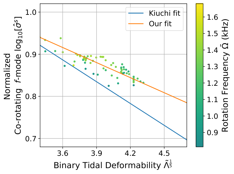
Without further constraints, this does not immediately lead to a universal relation. In fact, we observe a clear distinction between the soft and stiff EoSs (cf. Section II.2), and stars with low angular rotation rates also do not seem to fit very well into a single relation.
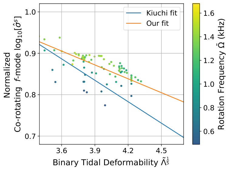
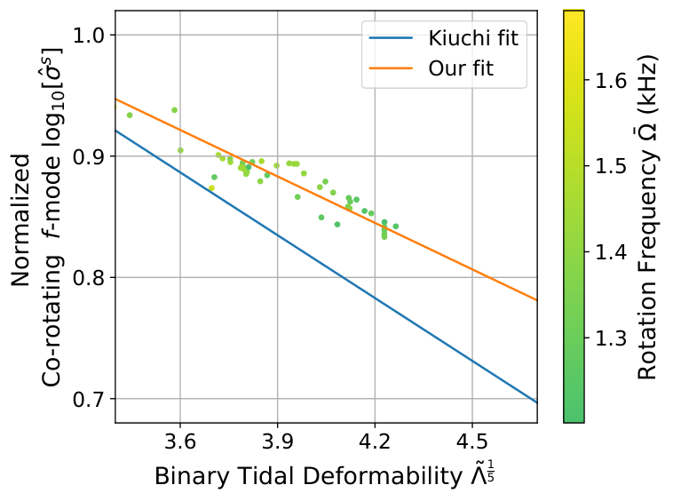
To remedy these issues, we add two constraints: first, since the EoSs used in Kiuchi et al. 2020 correspond mostly to the soft EoSs considered here, we, for now, ignore the stiff EoSs. Second, as we expect the remnant to be fast rotating, we require it to have a rotation frequency above a minimum rotation frequency threshold . While we considered a range of values for in our analyses, we here exemplarily discuss the result for . The corresponding figures for can be found in Appendix B.
The relation that includes the linear fit for stars with soft EoSs (i.e. APR4, SLy and WFF1) and rotation frequencies is shown in Figure 3. We can clearly observe a deviation from the relation put forward in Kiuchi et al. 2020 that is caused by us considering uniformly rotating neutron stars with cold EoSs (for a long-lived remnant), while the numerical relativity simulations performed in Kiuchi et al. 2020 include differential rotation and thermal corrections for the early post-merger remnants with hot EoSs. However, we are still able to reproduce the same functional form of the relation between and .
Generalizing this linear fit for arbitrary pre-merger mass ratios , we obtain a relation of the form
| (15) |
where
| (16) |
and
| (17) |
| 400 | ||||||||
| 800 | ||||||||
| 1200 |
The exact values of these coefficients for different rotation frequency thresholds are given in Table 1. We also give the RMSE and the average relative error of the estimated values for through Equation (15) compared to the original value (only considering stars with rotation frequency ). As one would expect, the higher the rotation frequency threshold is chosen, the more accurate the linear fit becomes. For instance, with , our linear fit achieves an RMSE of , and an average relative error of .
III.2 Counter-rotating -mode
Since we have access to the counter-rotating -mode of the rotating remnant neutron star, we also investigate the relation between the binary tidal deformability and the normalized and dimensionless counter-rotating -mode frequency
| (18) |
The superscript is used to indicate the potentially (CFS) unstable (i.e. counter-rotating) branch of the -mode for rotating stars. We again perform our analyses for different rotation frequencies and for different mass ratios . We also continue to only consider the soft EoSs (APR4, WFF1 and SLy), as before.
Since the counter-rotating -mode frequency can reach negative values, we cannot straightforwardly adapt the same form for our relation as above due to the logarithm used there. While there are several approaches one could take to alleviate this issue (e.g. ignore negative frequencies, or only consider the absolute value of the frequency), our evaluations have shown that the best results are achieved when one attempts a simple linear relation.
In Figure 4, we show the counter-rotating -mode against the binary tidal deformability, colored by the rotation frequency of the star. We can immediately see that a single, rotation independent relation is clearly out of reach. However, we do observe a clear separation of the points by said rotation frequency, suggesting a linear relation of the form
| (19) |
where
| (20) |
is the normalized angular rotation rate, and and are given by
| (21) |
| (22) |
where each of the -dependent coefficients is again a quadratic function of . Note that, while we did examine different parameterizations for the rotation rate, the normalized angular rotation rate proved to provide the best fit.

Our best fit for this relation is also illustrated in Figure 4 for . We also show our estimates for all of the data points, each indicated by an ‘’. The lines connecting corresponding pairs are shown in pink if the estimate is smaller than the actual value, and in green if the estimate is larger.
| 2 | 1 | 0 | |
|---|---|---|---|
The coefficients for this fit are listed Table 2. They have the form
| (23) |
This fit achieves an RMSE of within our data set, and an average relative error of . Note that the relative error is necessarily higher here as we have frequency values around zero. If we only compare the RMSE with the error for the co-rotating relation, we achieve similar accuracy (note that there we estimated the logarithm of the normalized -mode frequency). However, we now have a two-parameter fit, which is more difficult to utilize in practice, as in addition to an estimate for the mass ratio, we would also need an accurate estimate for the rotation frequency of the remnant.
Still, in cases where we are able to obtain accurate estimates for these two quantities for a BNS merger, we can use the relation presented here to predict whether we might observe, e.g., a CFS-instability in the remnant due to a negative counter-rotating -mode frequency Chandrasekhar 1970; Friedman and Schutz 1978; Doneva et al. 2015.
III.3 Combined Relation
Combining the linear fit in Equation (15) with the fit in (Krüger and Kokkotas 2020a, Equation (6)), we obtain a combined relation for the effective compactness of the form
| (24) |
where is again the normalized angular rotation rate (cf. Equation (20)) of the long-lived remnant, and the coefficients and are given in Krüger and Kokkotas 2020a. This relation allows us to estimate the effective compactness of the long-lived post-merger star from the tidal deformabilities of the pre-merger neutron stars.
A comparison of the estimated effective compactnesses through Equation (24) (shown as triangles) and the actual effective compactnesses (shown as dots) is illustrated in Figure 5. Again, lines connecting corresponding pairs are shown in pink if the estimate is smaller than the actual value, and in green if the estimate is larger.

The RMSE, average relative error and the maximum relative error for each rotation frequency threshold are given in Table 3. On average, we achieve a relative error of around .
Conceptually, we could formulate a similar relation using the counter-rotating -mode, as well. However, the combined relation presented here is only intended as a motivating starting point, and will be replaced by a direct relation in the next section. We therefore do not further detail this approach at this point.
IV Direct Universal Relations
After using the results presented in Section III and in Krüger and Kokkotas 2020a to derive a combined relation between the pre-merger binary tidal deformability and the effective compactness of the long-lived remnant via the -mode frequency, we now attempt a direct relation between these two quantities with the goal of achieving improved accuracy.
IV.1 Two-Parameter, Linear Relation
As with the combined relation in Section III.3, we begin by considering the EoSs that we call soft, i.e. WFF1, APR4 and SLy (cf. Section II.2). A good fit is achieved by comparing with . The resulting relation is illustrated in Figure 6.

We can observe a clear separation of the data points by the rotation frequency . After examining different rotation parameters, the normalized angular rotation rate (cf. Equation (24)) again proved to perform best in our fits. Ultimately, we reach a linear, two-parameter fit of the form
| (25) |
with
| (26) |
| (27) |
where each of the -dependent coefficients is again a quadratic function of .
The best fit of Equation (25) to our data is illustrated in Figure 6 for the case of . The errors incurred over all mass ratios are given in the first row of Table 6: the fit achieves an RMSE of , an average relative error of , and a maximum relative error of . The coefficients of this fit are listed in Table 4. They are defined as in Equation (23). The direct relation thus shows improved accuracy compared to the combined relation presented earlier: we go from an average relative error of to .
| 2 | 1 | 0 | |
|---|---|---|---|
With this improved accuracy, we can now also attempt to reintroduce the stiff EoSs (H4 and MS1) that we previously excluded for the combined relation. The resulting best fit is illustrated in Figure 7. Here, the data points for the stiff EoSs are indicated in red. This new fit for all EoSs achieves an RMSE of , an average relative error of , and a maximum relative error of . The coefficients of this fit can be found in Table 5. They are again defined as in Equation (23).
| 2 | 1 | 0 | |
|---|---|---|---|
As we can see, the direct relation admits the stiff EoSs with close to double the error. However, the error remains small and we achieve high accuracy even including stiff EoSs, thus improving the universality of our direct relation.
The inclusion of the stiff EoSs has a similar effect on the other relations we present below. For the sake of brevity, we will therefore present the results including only the soft EoSs in the remainder of the text, and refer to the appendix for the results with all EoSs.

| linear, two-parameter | |||
|---|---|---|---|
| quadratic, one-parameter | |||
| constrained |
IV.2 One-Parameter, Quadratic Relation
The plots in Figures 6 and 7 suggest that a one-parameter fit that only depends on the mass ratio , and is independent of the rotation frequency, might also be possible. We therefore attempt a relation of the form
| (28) |
where each of the coefficients and are quadratic in and take the form
| (29) |
The best fit of our data to this relation is shown in Figure 8. The coefficients corresponding to this fit are listed in Table 7 and the resulting errors in the second row of Table 6.
The quadratic fit performs only slightly worse than the linear, two-parameter fit, going from an average relative error of for the two-parameter fit, to for the one-parameter fit. However, it only depends on one free parameter, the mass ratio , and no longer on the rotation rate of the remnant. As such, the quadratic fit is preferable to the linear two-parameter fit in practice as we reduce the number of parameters that need to be estimated, while still achieving very similar accuracy.

IV.3 Compactness Relation
The compactness of neutron star has been the object of various universal relations considered in the past Andersson and Kokkotas 1998; Benhar et al. 2004; Tsui and Leung 2005; Chirenti et al. 2015. The advantage of an accurate universal relation that connects the binary tidal deformability of the BNS to the compactness of the long-lived remnant is that it allow us to directly constrain the remnant’s radius (using independent estimates for its gravitational mass), and through that its EoS. We therefore now investigate the possibility of such a relation.
We compute the compactness of the long-lived remnant through where is its equatorial radius.

After considering several options, we find that the best fit is obtained for a relation of the form
| (30) |
where the coefficients and have the same (quadratic) form as given in Equation (29).
The best fit for Equation (30) is illustrated in Figure 9. The coefficients of the best fit are given in Table 8.
| 2 | 1 | 0 | |
|---|---|---|---|
As we can see, the spread of the data points for the compactness relation is higher than for the effective compactness relations considered above. As listed in the first row of Table 9, the compactness relation achieves an RMSE of and an average relative error of . These errors are around an order of magnitude larger than for the effective compactness relations. Thus, the compactness relation clearly shows worse universality.
Despite the notably worse accuracy of the compactness relation, it might still be useful in practice by allowing us to directly constrain the remnant’s (equatorial) radius. Of course, the worse accuracy of this relation would also impact the accuracy of the radius constraints obtained in such a way.
V Relations with Constrained Rotation Rates
The universal relations discussed above allows for the full range of rotation frequencies of the long-lived remnant, from non-rotating up to the Keplerian limit. As such, imposing additional constraints to the remnant’s rotation rate appears to be a straightforward way to further improve the accuracy of our relations.
As we discussed in Section II, Radice et al. Radice et al. 2018a propose a universal relation for the spin-period of long-lived remnants (cf. Equation (13)) of BNS mergers, which they derived from numerical relativity simulations. We apply this universal relations here to our own long-lived remnants to constrain their rotation rates: given the baryon mass of the remnant, we only allow rotation rates that are predicted by Equation (13).
Through this, we end up with rotation frequencies around (depending on the remnant’s baryon mass). For our evaluations, we only consider neutron stars with rotation rates in a range around this value. In the following, we investigate how much the accuracy of the one-parameter relations for the effective compactness (cf. Section IV.2) and the compactness (cf. Section IV.3) relations improves by introducing this rotation rate constraint. We list the resulting errors for the effective compactness relation in the third row of Table 6, and for the compactness relation in the second row of Table 9.
Overall, this constraint only has a small impact on the accuracy of our relations: for the effective compactness relation, for instance, we go from an average relative error of from the quadratic relation without constraint (cf. second row of Table 6), to with constraint. We observe the largest change with the maximum relative error: it improves from without constraint, to with constraint.
The effect is similar for the compactness relation: the relative error again shows a slight improvement, from without constraint, to with constraint. The maximum relative error again shows a more significant improvement, going from for the unconstrained case, to in the constrained case, mirroring our observations for the effective compactness relation.
As such, we have found that introducing constraints on the free parameters in our relations can indeed improve the accuracy, albeit only slightly. Investigating how adding further constraints could more significantly improve our relations could be a fruitful direction for future work.
| unconstrained | |||
|---|---|---|---|
| constrained |
VI Mass Loss During Spin Down
Until now, we have assumed a negligible baryon mass loss going from the pre-merger neutron stars to the long-lived remnant of the merger. As we discussed in Section II, while the baryon mass loss during the merger is indeed negligible Bauswein et al. 2013; Hotokezaka et al. 2013; Sekiguchi et al. 2016; Radice et al. 2018b, Radice et al. Radice et al. 2018a put an upper bound of baryon mass lost during the spin down of the early, differentially rotating remnant to the long-lived, uniformly rotating remnant. Since this potential mass loss is substantial, we here revisit our universal relations for the effective compactness under the assumption that a baryon mass of is lost during the transition from the pre-merger stars to the long-lived remnant, i.e.
| (31) |
where is the baryon mass of the long-lived remnant, and and the baryon masses of the pre-merger stars.
Since we have a fixed data set of remnant configurations from Krüger and Kokkotas 2020a, we implement the mass loss by keeping the remnant configuration fixed, and instead increasing the masses of the pre-merger stars to account for the mass loss. We then recompute the solution of the TOV equations and the tidal deformability for this new set of pre-merger stars. In general, the inclusion of a non-negligible baryon mass loss will therefore cause a slight shift on the axis in Figures 6 to 9 as the increase of the pre-merger baryon masses will be reflected in a decrease of the binary deformability .
Since the effect of the mass loss is essentially the same for all of the universal relations presented in this paper, we here exemplarily only discuss the quadratic, one-parameter relation introduced in Section IV.2. We here also also only discuss the case of soft EoSs, and refer to Appendix C.3 for the case with all EoSs. However, the effect of including stiff EoSs is essentially the same as in the relations considered previously, and does not have any additional effect when combined with a non-negligible mass loss.
In the following, we first re-compute the new best fit of this relation to the new set of BNS merger data that assumes a baryon mass loss of , and present the resulting errors. Afterwards, we try to apply our original relation (without mass loss) to the mergers with mass loss and give an estimate of the error incurred if the original relation were used for such mergers.
VI.1 New Best Fits for Mergers with Mass Loss
| 0 | |||
The data points and new best fits of the quadratic, one-parameter relation for BNS mergers with and are shown in Figure 10. For the sake of comparison, we also show our original fit (without mass loss) as a dashed line.
As we can see, the inclusion of mass loss does not change the form of our relation, or invalidate their universality. While there is a shift of the data points caused by the different pre-merger masses, the same relation as previously can be constructed with very similar errors. We list the errors of the new best fits together with the errors of our original relation in Table 10. We increased the number of decimal places shown compared to previous tables to show when the first differences appear. Ultimately, there is effectively no change in the accuracy of the best fits with increasing mass loss.
| Mass Loss | |||
|---|---|---|---|
| 0 | |||
VI.2 Original Relation for Mergers with Mass Loss
We have seen above that the inclusion of a non-negligible baryon mass loss still allows us to construct universal relations between the pre-merger binary tidal deformability and the effective compactness of the long-lived remnant (assuming a good estimate for the actual baryon mass loss is known). We now estimate the error incurred by using the original relation (without mass loss) for the mergers with and baryon mass loss, respectively. We give the resulting errors in Table 11.
As one would expect, the accuracy of our original relation (without mass loss) decreases as the mass loss increases. However, even for the worst case of , our original relation remains fairly accurate: we achieve an average relative error of if we only consider soft EoSs, compared to for mergers without mass loss.
Consequently, the relations presented in the paper seem to be robust against limited mass losses during the post-merger phase at the range of as predicted by Radice et al. Radice et al. 2018a. Therefore, even if we are not able to further constrain the post-merger mass loss, our original relation will remain useful.
VII Discussion & Conclusion
In this paper, we proposed a novel approach to developing universal relations for BNS mergers using results from perturbative calculations instead of using full-fledged numerical relativity simulations.
Our approach is based on a simplified model for a BNS merger that results in a long-lived neutron star remnant: instead of performing a detailed simulation of the merger process, we individually consider the pre-merger phase, represented by two irrotational neutron stars, and the long-lived remnant, represented by a rapidly rotating neutron star. By comparing the neutron stars in these two phases, we then obtain relations connecting their properties.
Inspired by previous results by Kiuchi et al. Kiuchi et al. 2020, and using the results from Krüger and Kokkotas 2020a, we proposed a novel universal relation between the pre-merger binary tidal deformability and the effective compactness of the long-lived remnant with high accuracy, reaching average relative error of if we only conisder soft EoSs, and if we also include stiff EoSs.
Similarly, we find a novel universal relation between the pre-merger binary tidal deformability and the compactness of the long-lived remnants, however with larger average relative error of if we only consider soft EoSs (and with all EoSs).
We furthermore find that the impact of a non-negligible mass loss during the transition from the differentially rotating, early remnant to the uniformly, rotating long-lived remnant on our relations is small. In particular, we find that a) we can easily construct new universal relations if good estimates for the post-merger baryon mass loss is known, and b) even the original relations (without mass loss) we presented in this paper can be applied to mergers with non-negligible baryon mass loss (up to ) with only a slight increase in the average relative error.
As the binary tidal deformability can be constrained fairly well from the observation of the gravitational waves emitted during the pre-merger phase Flanagan and Hinderer 2008; Favata 2014, and as the spectrum of the pre-merger gravitational waves lie very well within the sensitivity range of current-generation GW detectors Rodriguez et al. 2014, the relations presented in this paper can be useful for predicting the stellar parameters of a potentially long-lived remnant produced by a BNS merger.
They can, in particular, be useful for further constraining the true EoS of neutron stars: for instance, as recently discussed by Greif et al. Greif et al. 2020, combining accurate estimates for the gravitational mass (found directly from the gravitational waves) and the moment of inertia (derived by using Equation (3) to estimate ), can put further constraints on the radius of the neutron star, and thus its EoS.
While we only used perturbative calculations for our analyses, they were not performed in a vacuum: numerical relativity simulations still play an important role in directing our efforts into the right direction. Not only were our efforts inspired by previous, simulation-based results by Kiuchi et al. Kiuchi et al. 2020, but also, by employing the universal relation for the remnant spin period put forward by Radice et al. Radice et al. 2018a, we were able to further constrain our universal relations to more physical rotation rates of the remnant, improving our accuracy, and reducing the number of free parameters. As such, the approach presented in this paper should mostly be considered supplementary to existing numerical relativity efforts.
Future Directions. As already mentioned in the introduction, our model for the BNS merger is markedly simple and does not cover all aspects and details relevant for the merger of two neutron stars. Our approach, however, can be freely extended to include more involved measures such as hot EoSs to model the remnant right after the merger before it cools down. As discussed in Section II, considering EoSs with phase transitions, specifically, will be an important direction for future work.
Of interest would also be to include differential rotation into our post-merger model and to compute the corresponding oscillation modes (and other stellar parameters). This task has already been performed for simple differential rotation models under various approximations, such as the Cowling approximation Yoshida et al. 2002; Krüger et al. 2010. However, a more comprehensive approach with a more accurate model of differential rotation, and the treatment of the oscillations modes without approximation, would be desirable.
Acknowledgements.
C.K. gratefully acknowledges financial support by DFG research Grant No. 413873357.Appendix A Equilibrium Model

In general, the metric of a non-rotating neutron star is given by
| (32) |
where the function fulfills the conditions
| (33) |
With the energy-momentum tensor of a perfect fluid
| (34) |
the metric can be determined by solving the Tolman-Oppenheimer-Volkoff (TOV) equations
| (35) |
| (36) |
| (37) |
through integration from the center of the neutron star to its surface. We determine the surface to be at the radius at which the pressure first reaches .
For the initial values, we set (and thus ). Given a central energy density , the corresponding central pressure can be determined by Equations (6) and (7).
Since we aim to evolve neutron stars with given gravitational masses and for a BNS of total mass , we need to specify the correct central density that results in these masses. For low to medium mass neutron stars, we use a simple bisection search to find the correct central density. Closer to the maximum mass limit, the bisection search usually fails, and we fall back to linearly searching through the full range of central densities.

Appendix B Combined Relation for Different Rotation Thresholds
Appendix C Direction Relations with all EoSs
We here present the results for the direct relation considering all of the EoSs we described in Section II.2: in addition to the soft EoSs (WFF1, APR4 and SLy) we considered in the main body of the paper, we now also include the stiff EoSs (H4 and MS1). Throughout all of the presented plots, the points corresponding to the stiff EoSs will be indicated in red.
Note that the linear, two-parameter relation with all EoSs was already discussed in Section IV.1. It’s errors are again given in the first row of Table 12.
| linear, two-param. | |||
|---|---|---|---|
| quadratic, one-param. | |||
| constr. |
C.1 Quadratic, One-Parameter Relation
We first revisit the quadratic, one-parameter relation discussed in Section IV.2, now with all EoSs. The relation is illustrated in Figure 13a. The coefficients of the best fit are given in Table 13 and the resulting errors are given in the second row of Table 12. We go from an average relative error of for the case with only soft EoSs, to now .

C.2 Compactness Relation for all EoSs
We here revisit the compactness relation discussed in Section IV.3, now for all EoSs. The relation is illustrated in Figure 13b, with the corresponding coefficients given in Table 14. The relation achieves an average relative error of once we introduce the stiff EoSs, which again is slightly worse than for the case with only soft EoSs, where we achieved .
C.3 Relations with Mass Loss for all EoSs
We finally also investigate the impact of a non-negligible mass going from the pre-merger stars to the long-lived remnant while considering soft and stiff EoSs. In Figure 14, we show the data points and new best fits for the quadratic, one-parameter relation, together with the original fit (without mass loss) represented as a dashed line.
In Table 15 we list the errors of the two new fits, and compare them to the old fit without mass loss. Clearly, the new fits are exactly as accurate as the old relations, similar to what we observed in the main part of the paper for the case of only soft EoSs.
In Table 16, we show how accurate our original relation (without mass loss) is when applied to mergers with mass loss. As with the case with only soft EoSs that we considered in the main body of the paper, the case with all EoSs also incurs a small decrease in the accuracy of our original relation with increasing mass loss, in the range of for the average relative error.
Consequently, the behavior of our relations when considering a non-negligible mass loss is identical, independent of whether we consider only soft or all EoSs.

| 0 | |||
| Mass Loss | |||
|---|---|---|---|
| 0 | |||
References
- et al. et al. (2017) B. P. A. et al., LIGO Scientific Collaboration, and Virgo Collaboration, Phys. Rev. Lett. 119, 161101 (2017).
- et al. et al. (2020) B. P. A. et al., LIGO Scientific Collaboration, and Virgo Collaboration, ApJ 892, L3 (2020).
- Andersson and Kokkotas (1996) N. Andersson and K. D. Kokkotas, Phys. Rev. Lett. 77, 4134 (1996).
- Kokkotas et al. (2001) K. D. Kokkotas, T. A. Apostolatos, and N. Andersson, MNRAS 320, 307 (2001).
- Rezzolla et al. (2018) L. Rezzolla, E. R. Most, and L. R. Weih, ApJ 852, L25 (2018).
- Most et al. (2018) E. R. Most, L. R. Weih, L. Rezzolla, and J. Schaffner-Bielich, Phys. Rev. Lett. 120, 261103 (2018).
- Bauswein et al. (2020) A. Bauswein, S. Blacker, V. Vijayan, N. Stergioulas, K. Chatziioannou, J. A. Clark, N.-U. F. Bastian, D. B. Blaschke, M. Cierniak, and T. Fischer, Phys. Rev. Lett. 125, 141103 (2020).
- Andersson and Kokkotas (1998) N. Andersson and K. D. Kokkotas, MNRAS 299, 1059 (1998).
- Benhar et al. (2004) O. Benhar, V. Ferrari, and L. Gualtieri, Phys. Rev. D 70, 124015 (2004).
- Yagi and Yunes (2017) K. Yagi and N. Yunes, Phys. Rep. 681, 1 (2017).
- Bernuzzi et al. (2015) S. Bernuzzi, T. Dietrich, and A. Nagar, Phys. Rev. Lett. 115, 091101 (2015).
- Rezzolla and Takami (2016) L. Rezzolla and K. Takami, Phys. Rev. D 93, 124051 (2016).
- Kiuchi et al. (2020) K. Kiuchi, K. Kawaguchi, K. Kyutoku, Y. Sekiguchi, and M. Shibata, Phys. Rev. D 101, 084006 (2020).
- Flanagan and Hinderer (2008) É. É. Flanagan and T. Hinderer, Phys. Rev. D 77, 021502 (2008).
- Favata (2014) M. Favata, Phys. Rev. Lett. 112, 101101 (2014).
- Vretinaris et al. (2020) S. Vretinaris, N. Stergioulas, and A. Bauswein, Phys. Rev. D 101, 084039 (2020).
- Dietrich et al. (2018) T. Dietrich, D. Radice, S. Bernuzzi, F. Zappa, A. Perego, B. Brueugmann, S. V. Chaurasia, R. Dudi, W. Tichy, and M. Ujevic, (2018), arXiv:1806.01625 [gr-qc] .
- Krüger and Kokkotas (2020a) C. J. Krüger and K. D. Kokkotas, Phys. Rev. Lett. 125, 111106 (2020a).
- Krüger and Kokkotas (2020b) C. J. Krüger and K. D. Kokkotas, Phys. Rev. D 102, 064026 (2020b).
- Chandrasekhar (1970) S. Chandrasekhar, Phys. Rev. Lett. 24, 611 (1970).
- Friedman and Schutz (1978) J. L. Friedman and B. F. Schutz, ApJ 221, 937 (1978).
- Radice et al. (2018a) D. Radice, A. Perego, S. Bernuzzi, and B. Zhang, MNRAS 481, 3670 (2018a).
- Bauswein et al. (2013) A. Bauswein, S. Goriely, and H. T. Janka, ApJ 773, 78 (2013).
- Hotokezaka et al. (2013) K. Hotokezaka, K. Kiuchi, K. Kyutoku, H. Okawa, Y.-i. Sekiguchi, M. Shibata, and K. Taniguchi, Phys. Rev. D 87, 024001 (2013).
- Sekiguchi et al. (2016) Y. Sekiguchi, K. Kiuchi, K. Kyutoku, M. Shibata, and K. Taniguchi, Phys. Rev. D 93, 124046 (2016).
- Radice et al. (2018b) D. Radice, A. Perego, K. Hotokezaka, S. A. Fromm, S. Bernuzzi, and L. F. Roberts, ApJ 869, 130 (2018b).
- Bauswein et al. (2019) A. Bauswein, N.-U. F. Bastian, D. B. Blaschke, K. Chatziioannou, J. A. Clark, T. Fischer, and M. Oertel, Phys. Rev. Lett. 122, 061102 (2019).
- Nandi and Pal (2021) R. Nandi and S. Pal, European Physical Journal Special Topics 10.1140/epjs/s11734-021-00004-4 (2021).
- Cromartie et al. (2020) H. T. Cromartie, E. Fonseca, S. M. Ransom, P. B. Demorest, Z. Arzoumanian, H. Blumer, P. R. Brook, M. E. DeCesar, T. Dolch, J. A. Ellis, R. D. Ferdman, E. C. Ferrara, N. Garver-Daniels, P. A. Gentile, M. L. Jones, M. T. Lam, D. R. Lorimer, R. S. Lynch, M. A. McLaughlin, C. Ng, D. J. Nice, T. T. Pennucci, R. Spiewak, I. H. Stairs, K. Stovall, J. K. Swiggum, and W. W. Zhu, Nature Astronomy 4, 72 (2020).
- Han and Steiner (2019) S. Han and A. W. Steiner, Phys. Rev. D 99, 083014 (2019).
- Read et al. (2009) J. S. Read, B. D. Lackey, B. J. Owen, and J. L. Friedman, Phys. Rev. D 79, 124032 (2009).
- Douchin and Haensel (2001) F. Douchin and P. Haensel, A&A 380, 151 (2001).
- Wiringa et al. (1988) R. B. Wiringa, V. Fiks, and A. Fabrocini, Phys. Rev. C 38, 1010 (1988).
- Akmal et al. (1998) A. Akmal, V. R. Pandharipande, and D. G. Ravenhall, Phys. Rev. C 58, 1804 (1998).
- Lackey et al. (2006) B. D. Lackey, M. Nayyar, and B. J. Owen, Phys. Rev. D 73, 024021 (2006).
- Müller and Serot (1996) H. Müller and B. D. Serot, in APS Meeting Abstracts, APS Meeting Abstracts (1996) p. E7.04.
- Hinderer (2009) T. Hinderer, ApJ 697, 964 (2009).
- Damour and Nagar (2009) T. Damour and A. Nagar, Phys. Rev. D 80, 084035 (2009).
- Binnington and Poisson (2009) T. Binnington and E. Poisson, Phys. Rev. D 80, 084018 (2009).
- Thorne and Campolattaro (1967) K. S. Thorne and A. Campolattaro, ApJ 149, 591 (1967).
- Hinderer (2008) T. Hinderer, ApJ 677, 1216 (2008).
- Stergioulas and Friedman (1995) N. Stergioulas and J. L. Friedman, ApJ 444, 306 (1995).
- Nozawa et al. (1998) T. Nozawa, N. Stergioulas, E. Gourgoulhon, and Y. Eriguchi, A&AS 132, 431 (1998).
- Stergioulas (1995) N. Stergioulas, Rapidly Rotating Neutron Star, gravity.phys.uwm.edu/rns/ (1995).
- Tassoul (2000) J. L. Tassoul, Cambridge Astrophysics Series 36 (2000).
- Gaertig and Kokkotas (2008) E. Gaertig and K. D. Kokkotas, Phys. Rev. D 78, 064063 (2008).
- Paschalidis and Stergioulas (2017) V. Paschalidis and N. Stergioulas, Living Reviews in Relativity 20, 7 (2017).
- Doneva et al. (2015) D. D. Doneva, K. D. Kokkotas, and P. Pnigouras, Phys. Rev. D 92, 104040 (2015).
- Tsui and Leung (2005) L. K. Tsui and P. T. Leung, Phys. Rev. Lett. 95, 151101 (2005).
- Chirenti et al. (2015) C. Chirenti, G. H. de Souza, and W. Kastaun, Phys. Rev. D 91, 044034 (2015).
- Rodriguez et al. (2014) C. L. Rodriguez, B. Farr, V. Raymond, W. M. Farr, T. B. Littenberg, D. Fazi, and V. Kalogera, ApJ 784, 119 (2014).
- Greif et al. (2020) S. K. Greif, K. Hebeler, J. M. Lattimer, C. J. Pethick, and A. Schwenk, ApJ 901, 155 (2020).
- Yoshida et al. (2002) S. Yoshida, L. Rezzolla, S. Karino, and Y. Eriguchi, ApJ 568, L41 (2002).
- Krüger et al. (2010) C. Krüger, E. Gaertig, and K. D. Kokkotas, Phys. Rev. D 81, 084019 (2010).