Jamming Detection with Subcarrier Blanking for 5G and Beyond in Industry 4.0 Scenarios

Security has been one of the main pillars driving the 3rd Generation Partnership Project (3GPP) design of the fifth generation (5G) of mobile communication systems. In fact, several security functionalities are available in 5G at the packet data convergence protocol (PDCP) and above layers to guarantee authentication, privacy and data integrity [1]. On the other hand, denial of service attacks in the form of radio jamming have been recently recognized as a major threat for the 5G deployment in Industry 4.0 scenarios, in particular with ultra-reliable low-latency communications (URLLC). As an example, while we can assume that no malicious device can be activated inside a factory, it might happen that a jammer stationed outside the plant blocks the transmission of some legitimate devices inside that plant. Such attack can cause large economic losses to the factory by interrupting the production. Moreover, besides these 5G Industry 4.0 use cases, jamming detection and mitigation has been recognized as an extremely relevant topic also for sixth generation (6G) technologies [2].

Jamming attacks have been known as a threat for communication and localization systems for many years, and jammers have been extensively used in the military context to degrade the effectiveness of enemy radars. Mainly for that reason, it is very simple and inexpensive nowadays to obtain a jammer that is capable of emitting high jamming power [3]. Furthermore, aside from simple devices that can generate narrow- or wide-bands radio frequency (RF) interference [4], there exist much smarter but still easily available jamming devices too [5]. This last type, a.k.a. as reactive jammers, are inactive while no legitimate transmission is happening, and then starts generating interference as soon as they sense some transmission on the channel, making them very difficult to be detected. Differently from other security aspects like authentication and privacy that can and are well managed at PDCP and above layers in 5G, jamming, as a form of malicious interference, can be handled at the physical layer. In fact, physical layer security mechanisms are expected to play an important role in 6G [6].

A fundamental difference exists between a legitimate interfering device and a jammer. A legitimate device creates interference while respecting the rules of the standard regulating communications in that band and several well-known techniques exist to deal with that type of interference. A jammer is a malicious device that intentionally attacks the system, also violating the regulatory and standardization rules, and its activity can be extremely dangerous [7]. For that reason, a jamming-resilient communication system needs to perform two tasks: a) detection, to understand that some network performance degradation happens because of a malicious jamming attack and not because of fading or some legitimate cellular interference, and b) mitigation, with the implementation of focused techniques to limit the impact of the attacker.

Here, we consider the problem of jamming detection in 5G-and-beyond communication systems, with particular focus on URLLC. Some work has recently been done in this framework. In [8], a detection technique has been proposed for massive multiple-input multiple-output (MIMO) base stations (BSs) exploiting pseudo-random hopping of the scheduled user equipments (UEs) among the pilot sequences and allowing the BS to design a jamming-resilient combiner. A more specific analysis for URLLC has been done by [9], where an advanced feedback is proposed and relays implementing promiscuous listening are used to detect rare events like a jammer. Along this direction, [10] proposes to deploy a guard node that generates and transmits a signal known at the legitimate receiver: the received signal is then post-processed to determine if a jamming attack occurred.

In this work we consider a system using orthogonal frequency division multiplexing (OFDM) and propose a novel method based on pseudo-random blanking of subcarriers to detect jamming attacks. Differently from [9, 10], our proposal does not require the deployment of additional nodes and, differently from [8], it applies also to the case of BSs with limited number of antennas, which occurs in particular with 5G deployments for Industry 4.0 indoor scenarios. Moreover, our proposal can be seamlessly embedded in the air interface design of OFDM-based technologies, including the long term evolution (LTE), 5G new radio (NR) and the anticipated 6G. More specifically, we design a detector exploiting the generalized likelihood ratio test (GLRT) and aiming to detect a smart jammer. Namely, we study a jammer with one of the following objectives: a) maximize the missed detection (MD) probability to remain stealthy, b) minimize the spectral efficiency (SE), assuming a mobile broadband (MBB) type of traffic, and c) maximize the block error rate (BLER), considering a URLLC type of traffic. The subcarrier blanking represents a loss in terms of system performance as some resources are not used for communication. Numerical results are provided to show the benefits of the proposed approach and the trade-off between the capability of detecting a jammer and the system performance.

Notation. $(\cdot)^{\textnormal{T}}$ denotes the transpose. $\lVert\textbf{X}\rVert$ is the Euclidean norm of X. $|\mathcal{X}|$ denotes the cardinality of the set $\mathcal{X}$.  $\overline{\hbox{}}$$\mathcal{X}$ denotes the complement of the set $\mathcal{X}$. $\textnormal{diag}(x_{1},\dots,x_{N})$ denotes the diagonal matrix where $x_{1},\dots,x_{N}$ are the diagonal elements. $C_{n,k}=\binom{n}{k}=\frac{n!}{k!(n-k)!}$ denotes the number of $k$-combinations from a given set of $n$ elements. $\mathcal{CN}(\mu,\sigma^{2})$ denotes the complex Gaussian distribution with mean $\mu$ and variance $\sigma^{2}$. $Q(\cdot)$ denotes the Gaussian Q-function. $P[A]$ denotes the probability of event $A$. $\mathbb{E}[X]$ denotes the expectation of random variable (r.v.) $X$.

We consider a single-cell single-user uplink scenario with a UE transmitting toward a BS; both UE and BS are single-antenna. Moreover, we assume a jammer that tries to disrupt the ongoing communication by sending a malicious signal to the BS. The considered system uses an OFDM modulation where the available radio resources can be thought as in a resource grid composed of resource elements (REs), where each RE occupies one subcarrier in frequency and one OFDM symbol in time, for a total of $S$ subcarriers per OFDM symbol (see also Fig. 1).

We now define the signal received by the BS on subcarrier $s\in\{1,\dots,S\}$ at symbol $n\in\mathbb{N}$ as

where $u_{s}(n)$ is the signal from the UE, $h_{s}(n)$ is the UE channel, $j_{s}(n)$ is the signal from the jammer, and $g_{s}(n)$ is the jammer channel. Moreover, $w_{s}(n)\sim\mathcal{CN}(0,\sigma_{w}^{2})$ is the complex Gaussian noise with $\sigma_{w}^{2}$ as statistical power. In particular, in this paper we consider two types of channel:

• •

  additive white Gaussian noise (AWGN) channel with $h_{s}(n)=H$ and $g_{s}(n)=G$, where $H$ and $G$ are constant for each subcarrier and OFDM symbol;

• •

  Rayleigh channel with $h_{s}(n)\sim\mathcal{CN}(0,\sigma_{h}^{2})$ and $g_{s}(n)\sim\mathcal{CN}(0,\sigma_{g}^{2})$.

We can now write the corresponding signal to interference plus noise ratio (SINR) on subcarrier $s\in\{1,\dots,S\}$ at symbol $n\in\mathbb{N}$ as

where $P_{\textnormal{UE},s}(n)$ is the UE power and $P_{\textnormal{J},s}(n)$ is the jammer power. We denote the respective total power per symbol as $P_{\textnormal{UE}}(n)=\sum_{s=1}^{S}P_{\textnormal{UE},s}(n)$ and $P_{\textnormal{J}}(n)=\sum_{s=1}^{S}P_{\textnormal{J},s}(n)$.

Regarding the key performance indicators (KPIs) that will be used to evaluate the damage caused by the jammer to the legitimate system, in this work we focus on SE and BLER. SE is most relevant when considering MBB type of traffic and we define it as

For what concerns the BLER, it comes in handy for evaluating the system performance in a URLLC type of traffic. In fact, in the URLLC case we assume that we have small packets sent by the UE, each packet scheduled on a set of REs allocated within a limited number of OFDM symbols: because of the tight latency constraint of URLLC, we do not assume retransmission capabilities. For our analysis, we define a certain $\textnormal{SINR}_{\textnormal{pkt}}$ as the equivalent SINR experienced by a packet (which can be computed by using different link-to-system mapping criteria [11]), and using this we compute the BLER from the normal approximation of the finite blocklength capacity:

where $V$ is the channel dispersion, $\rho$ is the packet spectral efficiency, and $C$ is the coded packet size [12, Eq. (5)].

In this work, we propose to blank some REs in each OFDM symbol in a pseudo-random manner, such that the attacker cannot predict in advance which resources will be used for transmission and which will be blanked. With our proposal, we have then two types of REs: data REs and blanked REs. The former is used for data transmission, while the latter is, indeed, left blanked and will be used for jamming detection. In particular, at each OFDM symbol $n$, the UE blanks a set $\mathcal{M}(n)=\{m_{1}(n),\dots,m_{M}(n)\}$ (with cardinality $M=|\mathcal{M}(n)|$) of REs, where $m_{1}(n),\dots,m_{M}(n)$ are chosen in a pseudo-random manner from the set $\{1,\dots,S\}$; the remaining REs are used for data transmission. Since no data is transmitted on the blanked REs, we define the UE signal introduced in (1) as

where $d_{s}(n)$ is the data sample sent by the UE. At the same time, the attacker transmits on a set $\mathcal{L}(n)=\{\ell_{1}(n),\dots,\ell_{L}(n)\}$ (with cardinality $L=|\mathcal{L}(n)|$) of REs, where $\ell_{1}(n),\dots,\ell_{L}(n)$ are chosen from the set $\{1,\dots,S\}$ according to the jammer strategy. Note that while here we consider mainly for sake of notation $M$ and $L$ constant, in practice they can also be discrete random variables. Fig. 1 shows an example of the resource grid in such situation.

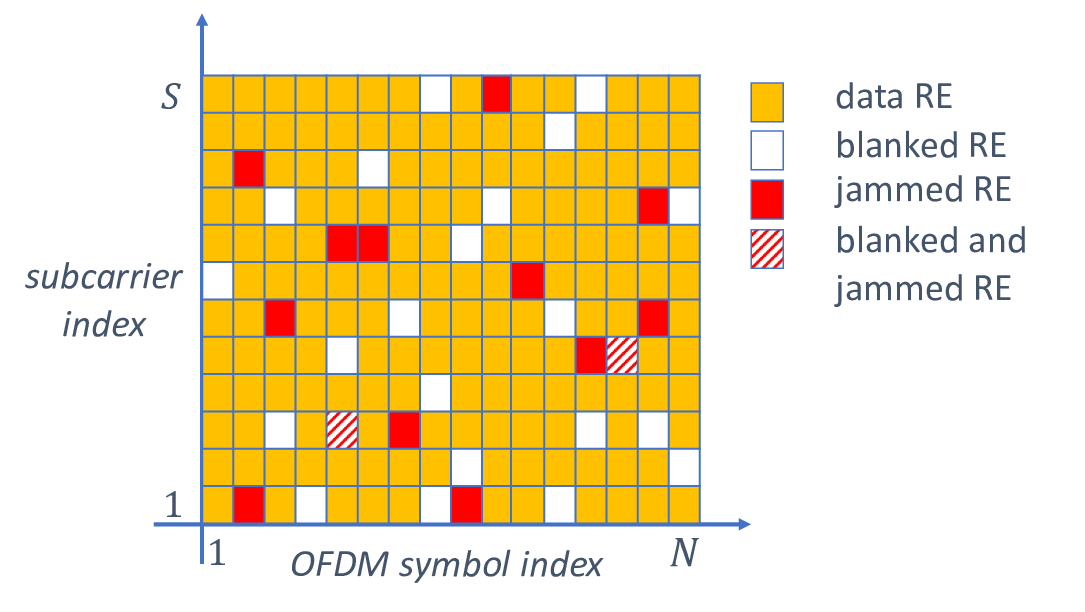
The defense strategy takes advantage of the blanked REs to detect the presence of jamming by means of statistical hypothesis testing [13]. The two hypotheses for the sequence of blanked REs are as follows:

• •

  There is no jamming and we have just thermal noise (null hypothesis $\mathcal{H}_{0}$);

• •

  There is jamming (alternative hypothesis $\mathcal{H}_{1}$).

Although we consider here a single-cell scenario, this method can be extended to the case with multiple BSs that share the same sequence of REs to be blanked. That is particularly beneficial for instance in Industry 4.0 scenarios in the several countries where specific bands are now being allocated to industry players for deploying their own 5G-and-beyond network without interference from neighbouring networks [14].

By denoting with $N$ the number of OFDM symbols that will be used at the BS for jamming detection, the above hypotheses translate in the following hypothesis test:

where $\mathbf{r}=\left[r_{m_{1}(1)}\cdots r_{m_{M}(1)}\cdots r_{m_{1}(N)}\cdots r_{m_{M}(N)}\right]^{\textnormal{T}}$, $\mathbf{w}=\left[w_{m_{1}(1)}\cdots w_{m_{M}(1)}\cdots w_{m_{1}(N)}\cdots w_{m_{M}(N)}\right]^{\textnormal{T}}$, and $\mathbf{j}=\left[j_{m_{1}(1)}\cdots j_{m_{M}(1)}\cdots j_{m_{1}(N)}\cdots j_{m_{M}(N)}\right]^{\textnormal{T}}$. These are vectors containing the samples of all the blanked REs for, respectively, received, noise, and jamming signal. Moreover, $\mathbf{G}=\textnormal{diag}(g_{m_{1}(1)},\dots,g_{m_{M}(1)},\dots,g_{m_{1}(N)},\dots,g_{m_{M}(N)})$ is the jammer channel matrix.

After defining the received jamming signal as $\tilde{\mathbf{j}}=\mathbf{G}\mathbf{j}$, we propose here a detector in the most general case where no assumption can be made about $\tilde{\mathbf{j}}$. Then, in Section IV, we use the derived detector for computing the MD probability in closed form in the case that $\tilde{\mathbf{j}}$ has zero-mean complex Gaussian distribution.

By assuming that the statistics of the jamming signal received by the BS are unknown, $\mathcal{H}_{1}$ becomes a composite alternative hypothesis and we need to resort to the GLRT [13]. The GLRT decides for $\mathcal{H}_{1}$ if

where $p(\mathbf{r};\mathcal{H}_{0})$ is the probability density function (PDF) of $\mathbf{r}$ under $\mathcal{H}_{0}$ and $p(\mathbf{r}|\hat{\mathbf{j}};\mathcal{H}_{1})$ is the PDF of $\mathbf{r}$ conditioned on $\tilde{\mathbf{j}}=\hat{\mathbf{j}}$ and under $\mathcal{H}_{1}$. Moreover, $\hat{\mathbf{j}}$ is the maximum likelihood estimate (MLE) of $\tilde{\mathbf{j}}$ assuming $\mathcal{H}_{1}$ is true, $\Lambda(\mathbf{r})$ is the test statistic, and $\lambda$ is the threshold. In particular, $\lambda$ is found from

where $P_{\textnormal{FA}}$ is the false alarm (FA) probability, i.e., the probability of declaring jamming even if it is not present.

We now derive the threshold $\lambda$ by fixing the value of $P_{\textnormal{FA}}$. First of all, we need to compute the test statistic formula, and we start by deriving the PDF of $\mathbf{r}$ under $\mathcal{H}_{0}$ and $\mathcal{H}_{1}$. When $\mathcal{H}_{0}$ is true, the signal received at the BS is $\mathbf{r}=\mathbf{w}$, therefore, we have $\mathbf{r}\sim\mathcal{CN}(\mathbf{0},\sigma_{w}^{2}\mathbf{I})$. When $\mathcal{H}_{1}$ is true, the received signal becomes $\mathbf{r}=\mathbf{w}+\tilde{\mathbf{j}}$, where $\tilde{\mathbf{j}}$ is an unknown vector, with resulting distribution $\mathbf{r}\sim\mathcal{CN}(\tilde{\mathbf{j}},\sigma_{w}^{2}\mathbf{I})$. In order to derive the corresponding PDF, we need to compute the MLE of $\tilde{\mathbf{j}}$ by maximizing $p(\mathbf{r}|\tilde{\mathbf{j}};\mathcal{H}_{1})$ through the following optimization problem:

Under our assumptions, the solution is just $\hat{\mathbf{j}}=\mathbf{r}$, thus leading to

By applying (10) to (7) and after some computations, the resulting decision rule can be rewritten as

with $\Lambda^{\prime}(\mathbf{r})\triangleq\frac{\sigma_{w}^{2}\ln{\Lambda(\mathbf{r})}}{MN}$ being the new test statistic and $\lambda^{\prime}\triangleq\frac{\sigma_{w}^{2}\ln{\lambda}}{MN}$ the new threshold. This is, basically, an energy detector, which is quite an intuitive result: when we have no knowledge about the jamming signal, we can just compute the energy of the received signal on the blanked REs and compare it against a thereshold.

The test statistic distribution under $\mathcal{H}_{0}$ is then

where $\textnormal{Gamma}(k,\theta)$ is the gamma distribution with shape paramenter $k$ and scale parameter $\theta$. From (8), the resulting FA probability turns out to be

where $F_{X}(x)$ denotes the cumulative distribution function (CDF) of the r.v. $X$ computed in $x$. This leads to

which can be now used to evaluate the detection performance of this defense strategy. This is done by means of the MD probability, defined as the probability of accepting $\mathcal{H}_{0}$ when jamming is present. In this model, the test statistic distribution under $\mathcal{H}_{1}$ can be written as

where $\chi^{2}(\nu,\delta)$ is the non-central $\chi^{2}$ distribution with $\nu$ degrees of freedom and non-centrality parameter $\delta$. Eventually, we can write the MD probability as

We now evaluate the effectiveness of the proposed defense strategy against a jamming signal with distribution $\tilde{\mathbf{j}}\sim\mathcal{CN}\left(\mathbf{0},\mathbf{D}\right)$, where $\mathbf{D}=\textnormal{diag}(d_{m_{1}(1)},\dots,d_{m_{M}(1)},\dots,d_{m_{1}(N)},\dots,d_{m_{M}(N)})$ is the covariance matrix with diagonal elements defined as

with $P_{\textnormal{J}}$ the jamming power per symbol, $i=1,\dots,M$, and $n=1,\dots,N$. In order to evaluate the performance of this type of attack against the defense mechanism, we apply the decision rule defined in (11) and we compute in closed form the corresponding MD probability. This result, besides for the analysis purpose, will be useful in Section V when deriving the best jammer strategy for minimizing its detectability.

For this computation, we need to take into account that the MD probability at a given time depends on the number of jammed REs that falls into the blanked ones. Therefore, first of all, we define the set $\mathcal{E}=\left[\mathcal{M}(1)\cap\mathcal{L}(1)\right]\cup\dots\cup\left[\mathcal{M}(N)\cap\mathcal{L}(N)\right]=\{e_{1},\dots,e_{E}\}$ (with cardinality $E=|\mathcal{E}|$) of overlapping blanked and jammed REs. Then, by denoting with $\widetilde{\Lambda}^{\prime}(\mathbf{r},E;\mathcal{H}_{1})$ the test statistic under $\mathcal{H}_{1}$ in (15) with the new assumption of Gaussian jammer, the MD probability can be computed as

where the law of total probability has been applied. Moreover,

are the minimum and maximum number of overlapping REs, given $M$, $L$, and $S$. We now need to derive the two factors in (17), i.e., the CDF of the test statistic under $\mathcal{H}_{1}$ and the probability mass function (PMF) of $E$.

Starting from the former, the test statistic distribution under $\mathcal{H}_{1}$, after some computations, results in

where $\mathcal{E}(1/\beta)$ is the exponential distribution with rate parameter $1/\beta$. To derive its CDF, we take advantage of a result in [15, Eq. (9)] on the CDF of the sum of independent exponential r.v.s:

where $\alpha_{1}=E$, $\alpha_{2}=MN-E$, $\beta_{\langle 1\rangle}=\frac{\sigma_{w}^{2}+\sigma_{j}^{2}}{MN}$, $\beta_{\langle 2\rangle}=\frac{\sigma_{w}^{2}}{MN}$, and

with $b\neq i$ and $\omega_{i,j}=\alpha_{i}-j$.

Finally, we observe that $E$ is a hypergeometric random variable, whose PMF can be written as

where

• •

  $C_{SN,MN}$ is the number of ways to choose $MN$ total blanked subcarriers out of $SN$ total subcarriers;

• •

  $C_{(S-L)N,MN-e}$ is the number of ways to choose $MN-e$ blanked subcarriers ($e$ overlapping subcarriers are fixed) out of $(S-L)N$ subcarriers ($LN$ jammed subcarriers are fixed);

• •

  $C_{LN,e}$ is the number of ways to choose $e$ overlapping subcarriers out of $LN$ total jammed subcarriers.

A jammer has the two tasks of a) not being detected and b) minimize the system performance. Since expressing an optimization problem that considers both tasks at the same time is not trivial , we consider in this work the following three heuristic strategies in order to achieve the above objectives:

• •

  maximize the MD probability, to remain as much undetected as possible, but still transmitting at maximum power;

• •

  minimize the SE, to reduce the performance with MBB type of traffic;

• •

  maximize the BLER, to disrupt a URLLC type of traffic.

Before going through all of them, we first make some assumptions on the jammer knowledge of the system. While it is fair that the jammer knows or can estimate many parameters (either because defined by the standard or just because it can listen to BS and UE transmission), some variables cannot be easily tracked by the attacker, like the instantaneous channel between the UE and the BS. Therefore, in general, we assume the jammer to know the format of the transmission, the large scale fading, and the noise statistical power at the BS. Moreover, regarding the defensive parameters, it is reasonable to assume that the jammer knows the number of blanked REs $M$, by estimating it (since we consider it fixed in time), and the number of symbols $N$ that the defense strategy uses for detection.

We consider an OFDM system with $S=300$ subcarriers, compliant to a 5G numerology with $60\,\textnormal{kHz}$ as subcarrier spacing for a $20\,\textnormal{MHz}$ bandwidth. The subcarriers are grouped into physical resource blocks (PRBs), each consisting of $S_{P}=12$ consecutive subcarriers, and transmission happens in slot of $14$ OFDM symbols [1]. Therefore, we have $P=S/S_{P}=25$ PRBs per slot, and we assume the detection to be performed per slot, i.e., $N=14$. As the PRB is the smallest time-frequency resource that can be scheduled to a device, we implement a 5G standard compliant defense with blanking performed per PRB and, as a consequence, introduce $M_{P}$ as the number of blanked PRBs per slot. For simplicity, we also assume the jammer to perform attacks on a PRB basis and denote with $L_{P}$ the number of jammed PRBs per slot.

We introduce now some parameters to better define the considered simulation setup:

• •

  $\textnormal{SNR}_{\textnormal{UE}}(n)=P_{\textnormal{UE}}(n)/(S\cdot\sigma_{w}^{2})$ is the UE signal to noise ratio (SNR) at OFDM symbol $n$, where $P_{\textnormal{UE}}(n)$ is the power that the UE allocates at symbol $n$ and evenly distributes among the data subcarriers; in our simulations we set $\textnormal{SNR}_{\textnormal{UE}}=10\,\textnormal{dB}$;

• •

  $\textnormal{SNR}_{\textnormal{J}}(n)=P_{\textnormal{J}}(n)/(S\cdot\sigma_{w}^{2})$ is the jammer SNR at OFDM symbol $n$, where $P_{\textnormal{J}}(n)$ is the power that the jammer allocates at symbol $n$ and evenly distributes among the jammed subcarriers.

Moreover, for the Rayleigh case, we consider a block fading model and assume different channel realizations on different PRBs. For URLLC type of traffic, we consider one packet per PRB, with $\rho=0.48\,\textnormal{bit/s/Hz}$.

Let’s start with the performance evaluation of the defense strategy, in terms of MD probability as a function of the FA probability, a.k.a. receiver operating characteristic (ROC) curve. Fig. 2 shows the ROC for $M_{P}=1,5$, $L_{P}=5,21$ (an almost narrow- and an almost wide-band jammer), $\textnormal{SNR}_{\textnormal{J}}=0\,\textnormal{dB}$, and for both AWGN and Rayleigh. First, we notice a huge performance improvement when using $M_{P}=5$ when compared to $M_{P}=1$, especially with $L_{P}=21$ subcarriers and AWGN: in fact, while with $M_{P}=1$ the MD is almost always above $10^{-1}$ for the considered range of target FA, with $M_{P}=5$ the detection performance strongly improves. Moreover, we also observe that while the narrow-band jammer ($L_{P}=5$) is hardly detectable, the wide-band one can be easily spotted by the proposed method even if we have small jamming power. Finally, results show that detection in a AWGN scenario is far easier when compared to detection in a more random channel like the Rayleigh considered here.

To evaluate the performance degradation with a MBB type of traffic, Fig. 3 shows the SE as a function of $\textnormal{SNR}_{\textnormal{J}}$ with $M_{P}=5$, for the almost narrow- and almost wide-band attack, and for a system with no blanking and no jamming that provides an upper bound to the proposed method. First, we notice, as expected, a small performance loss of the proposed method against the upper bound at very low jamming power because of the PRB blanking. Moreover, while the wide-band attack causes significant SE loss, especially for high $\textnormal{SNR}_{\textnormal{J}}$, the narrow-band attack, that resulted in Fig. 2 to be more stealthy, only slightly limits the system SE.

Concerning the URLLC type of traffic, Fig. 4 shows the BLER as a function of $\textnormal{SNR}_{\textnormal{J}}$ for $L_{P}=5,21$ jammed PRBs and $M_{P}=5$ blanked PRBs. In the AWGN channel, we observe that with limited jamming power, a narrow-band attack allows the jammer to strongly degrade the performance and at the same time avoid the blanked PRBs. But, as its power increases, the BLER reaches a saturation value, which depends on the probability of intersection between blanked and jammed PRBs, and for higher $\textnormal{SNR}_{\textnormal{J}}$ it should switch to a wide-band attack. When looking at the Rayleigh case, we observe that, in general, the system performs worse than the AWGN case.

In Fig. 5 we evaluate the jammer strategy for MD maximization proposed in Section V-A by showing for $\textnormal{SNR}_{\textnormal{J}}=-10,0\,\textnormal{dB}$ the best MD probability achievable by the attacker and the corresponding number of jammed PRBs to achieve it. For the low power jammer, i.e., $\textnormal{SNR}_{\textnormal{J}}=-10\,\textnormal{dB}$, we notice that if the defender’s target FA probability is $P_{\textnormal{FA}}\gtrsim 10^{-4}$, the best approach for the jammer is to perform a narrow-band attack; this happens because the defense tends to accept the $\mathcal{H}_{1}$ hypothesis more easily, and therefore the attacker tries to avoid the blanked PRBs by transmitting on a smaller number of PRBs. On the other hand, for $P_{\textnormal{FA}}\lesssim 10^{-4}$, the jammer best strategy is a wide-band attack because, in this way, it evenly distributes its power among all the subcarriers. On the contrary, with a higher jamming power, i.e., $\textnormal{SNR}_{\textnormal{J}}=0\,\textnormal{dB}$, we see that the optimal strategy is the narrow-band attack for the entire FA probability interval that we consider.

In Section V-B we showed that the best strategy to minimize the SE is a wide-band attack, while in Fig. 5 we learned that, on the contrary, in many cases the narrow-band attack is the best strategy to maximize the MD, thus suggesting a trade-off between MD probability and SE. In Fig. 6 we evaluate this trade-off by showing the MD probability versus the SE, for different values of $L_{P}$ and $\textnormal{SNR}_{\textnormal{J}}$, and for $P_{\textnormal{FA}}=10^{-3}$. The optimal situation for the attacker would be to achieve high $P_{\textnormal{MD}}$ and low SE, but, for the considered range of $\textnormal{SNR}_{\textnormal{J}}$, there is a maximum that can be achieved and, depending on its objective, the jammer needs to give up on SE reduction if it wants to increase the MD and viceversa.

Finally, Fig. 7 considers the BLER maximization problem of Section V-C and shows the MD probability versus the BLER, for different values of $L_{P}$ and $\textnormal{SNR}_{\textnormal{J}}$, and for $P_{\textnormal{FA}}=10^{-3}$. These results show that if the jammer has low power, for instance with $\textnormal{SNR}_{\textnormal{J}}=0\,\textnormal{dB}$, it cannot achieve high BLER and at the same time stay undetected. On the other hand, by looking at the top-right region of the plot, we observe that a jammer with a sufficiently high power can use a narrow-band attack to achieve high BLER and high $P_{\textnormal{MD}}$.

In this paper, we considered the problem of jamming detection for 5G-and-beyond in Industry 4.0 scenarios and designed a method based on pseudo-random blanking of subcarriers in an OFDM system. We then considered a smart jammer following three types of strategies: remain as stealthy as possible, maximize the damage to MBB communication, and maximize the disruption of URLLC type of traffic. Results show that, while for a MBB traffic the jammer has to compromise between MD and SE, with URLLC traffic, a smart jammer with sufficiently high power can achieve good results in reaching both high values of MD probability and BLER. Future works include performance evaluations in a 3GPP compliant Industry 4.0 scenario.

References

- [1] E. Dahlman, S. Parkvall, and J. Skold, 5G NR: the next generation wireless access technology. Academic Press, 2018.
- [2] H. Viswanathan and P. E. Mogensen, “Communications in the 6G era,” IEEE Access, vol. 8, pp. 57 063–57 074, 2020.
- [3] (2021) Jammer-store. [Online]. Available: http://www.jammer-store.com
- [4] W. Xu, K. Ma, W. Trappe, and Y. Zhang, “Jamming sensor networks: attack and defense strategies,” IEEE Netw., vol. 20, no. 3, pp. 41–47, May-Jun. 2006.
- [5] M. Wilhelm, I. Martinovic, J. B. Schmitt, and V. Lenders, “Short paper: Reactive jamming in wireless networks: How realistic is the threat?” in Proc. ACM Conference on Wireless Network Security (WiSec), Hamburg (Germany), Jun. 2011.
- [6] A. Chorti et al., “Context-aware security for 6G wireless: the role of physical layer security,” https://arxiv.org/abs/2101.01536, Jan. 2021.
- [7] C. Orakcal and D. Starobinski, “Rate adaptation in unlicensed bands under smart jamming attacks,” in Proc. ICST Conference on Cognitive Radio Oriented Wireless Networks and Communications (CROWNCOM), Stockholm (Sweden), Jun. 2012.
- [8] T. T. Do, E. Björnson, E. G. Larsson, and S. M. Razavizadeh, “Jamming-resistant receivers for the massive MIMO uplink,” IEEE Trans. Inf. Forensics Security, vol. 13, no. 1, pp. 210–223, Jan. 2018.
- [9] V. N. Swamy et al., “Monitoring under-modeled rare events for URLLC,” in Proc. IEEE International Workshop on Signal Processing Advances in Wireless Communications (SPAWC), Cannes (France), Jul. 2019.
- [10] P. Zhang and S. Sun, “One node to guard all: jamming-resistant and low-latency communication for IoT,” in Proc. IEEE Global Communications Conference (GLOBECOM), Abu Dhabi (UAE), Dec. 2018.
- [11] K. Brueninghaus et al., “Link performance models for system level simulations of broadband radio access systems,” in Proc. IEEE International Symposium on Personal, Indoor and Mobile Radio Communications (PIMRC), Berlin (Germany), Sep. 2005.
- [12] G. Durisi, T. Koch, and P. Popovski, “Toward massive, ultrareliable, and low-latency wireless communication with short packets,” Proc. IEEE, vol. 104, no. 9, pp. 1711–1726, Sep. 2016.
- [13] S. M. Kay, Fundamentals of statistical signal processing: detection theory. Prentice Hall, 1993.
- [14] Bundesnetzagentur, “Verwaltungsvorschrift für Frequenzzuteilungen für lokale Frequenznutzungen im Frequenzbereich 3.700-3.800 MHz (VV Lokales Breitband),” Nov. 2019.
- [15] T. V. K. Chaitanya and E. G. Larsson, “Optimal power allocation for hybrid ARQ with chase combining in i.i.d. rayleigh fading channels,” IEEE Trans. Commun., vol. 61, no. 5, pp. 1835–1846, May 2013.