Universal resource-efficient topological measurement-based quantum computation via color-code-based cluster states

We first present 2D color-code lattices on which CCCSs are based. We consider a lattice $\mathcal{L}_{2D}$ on a 2D plane which is 3-valent and has 3-colorable faces; namely, three edges meet at each vertex and one of the three colors (red, green, or blue) is assigned to each face in such a way that neighboring faces have different colors. Note that each edge, called link, is also colorable with the color of the faces it connects. Two typical examples (4-8-8 and 6-6-6) of such lattices are shown in Fig. 2. In the original 2D color codes, a qubit is attached to each vertex and two SGs ($X$- and $Z$-type) correspond to each face. Details on the codes are described in Ref. Bombin and Martin-Delgado 2006; Bombín 2013.

Regarding a color-code lattice $\mathcal{L}_{2D}$, three shrunk lattices are defined, one for each color by shrinking all the faces of that color, as shown in Fig. 3. For example, in the red shrunk lattice, each vertex corresponds to a red face in $\mathcal{L}_{2D}$ and each face corresponds to a blue or green face in $\mathcal{L}_{2D}$. Edges of the red shrunk lattice then correspond to red links in $\mathcal{L}_{2D}$. The blue and green shrunk lattices are also defined analogously.

The graph $G$ for a CCCS based on a color-code lattice $\mathcal{L}_{2D}$ has a 3D structure composed of multiple identical 2D layers stacked along the simulating time ($t$) axis. The layer of $t=t_{0}$ is referred to as the $t_{0}$-layer.

The structure of each layer is originated from $\mathcal{L}_{2D}$, as illustrated in Fig. 4(a) for the case of the 4-8-8 lattice. Each vertex in the layer is located at either a vertex of $\mathcal{L}_{2D}$ or the center of a face of $\mathcal{L}_{2D}$; the corresponding qubit is called a code qubit (CQ) or an ancilla qubit (AQ), respectively. Each AQ is colorable with the color of the corresponding face in $\mathcal{L}_{2D}$. For each face in $\mathcal{L}_{2D}$, the layer has an edge connecting the corresponding AQ and each surrounding CQ, on which a cz gate is applied. Each pair of CQs connected by a link in $\mathcal{L}_{2D}$ is called link here as well. Note that links are not edges of $G$.

Next, we stack multiple identical layers along the time axis as shown in Fig. 4(b). Every pair of CQs adjacent along the time axis is connected by an edge in $G$. The vertices (CQs and AQs) and edges (between CQs and AQs in the same layer and between CQs in the adjacent layers) constructed above finally complete the graph $G$ of the cluster state.

We assign each layer, qubit or link a “primality”: either primal or dual. Each layer is primal (dual) if it has an even (odd) time. An AQ is primal (dual) if it is in a primal (dual) layer, while a CQ or link is primal (dual) if it is in a dual (primal) layer. We label each qubit or link in an abbreviated form with its primality (“p” for primal and “d” for dual), color (“r” for red, “g” for green, and “b” for blue; omitted for CQs), and type (“AQ,” “CQ,” and “L” for a link). For example, a pgAQ means a primal green ancilla qubit. We also frequently use “c” instead of a specific color (r, g, or b) for a variable on colors.

We now present stabilizer generators (SGs) of a CCCS. Remark that, for each vertex $v$ in $G$, $S(v)$ given in Eq. (1) is a SG if $Q(v)$ is initialized to $\ket{+}$. We define A- and C-type SGs shown in Fig. 5(a) and (b) as follows.

The support ²² 2 The support of an operator $O$, written as $\mathrm{supp}(O)$, is the set of qubits on which $O$ applies non-trivially. of a C-type SG is distributed in three adjacent layers, while that of an A-type SG is contained in a layer.

Although these two types of SGs completely generate the stabilizer group, we need another two types of SGs: L- and J-type SGs in Fig. 5(c) and (d).

A-, L-, and J-type SGs together generate the stabilizer group over-completely. To see this, regarding a J-type SG $S_{I}$, we consider an L-type SG $S_{Li}:=S_{0}S_{i}$ for each $i\in\quantity{ 0, 1, 2, 3 }$, where $S_{i}$’s are defined in Definition 3. Then $S_{0}=S_{L1}S_{L2}S_{L3}S_{I}$ holds, thus any C-type SG can be written as the product of L- and J-type SGs.

Let the $P$-support $\mathrm{supp}_{P}(O)$ of a multi-qubit Pauli operator $O$ for $P\in\quantity{ X, Y, Z }$ be the subset of $\mathrm{supp}(O)$ corresponding to the $P$ operator. Note that, for every SG regardless of its type, qubits in its $X$- and $Z$-support always have different primalities.

Almost every discussion from now on is symmetric between the two primalities. Thus, throughout the rest of this paper, we frequently discuss only one of them, which implies that the other side can be treated similarly.

We now construct the shrunk lattices of a CCCS, which are analogous to those of the 2D color codes in Fig. 3. We then define correlation surfaces Raussendorf et al. 2006; Raussendorf and Harrington 2007; Raussendorf et al. 2007 within each shrunk lattice, through which logical gates are built for MBQC.

The primal c-colored shrunk lattice $\mathcal{L}^{\textup{{pc}}}$ is a 3D lattice containing every pcAQ as a vertex. Note that the vertices are only in primal layers. There are two types of edges connecting them: “spacelike” and “timelike” edges. Each spacelike edge corresponds to a pcL and connects two vertices in a layer. Each timelike edge connects two vertices adjacent along the time axis and contains a dcAQ between them. Faces and cells are then naturally defined by the vertices and edges. Cells in each primal shrunk lattice are visualized in Fig. 6 for 4-8-8 CCCSs. Note that each primal layer in $\mathcal{L}^{\textup{{pc}}}$ is identical with the c-colored shrunk lattice of the 2D color code on which the CCCS is based.

Each element (vertex, edge, face, or cell) in a shrunk lattice corresponds to an AQ or a link, as presented in Table 1. Here $Q(b)$ for an element $b$ denotes the set of qubits corresponding to $b$. Note that an element is colorable with the color of AQ or link corresponding to it. In particular, cells and spacelike faces have colors different from the color of the shrunk lattice, e.g., $\mathcal{L}^{\textup{{pr}}}$ is composed of green and blue cells.

We now regard the shrunk lattices as chain complexes Raussendorf et al. 2006; Raussendorf and Harrington 2007; Raussendorf et al. 2007. Let $\mathcal{B}_{i}^{\textup{{pc}}}$ for $i=0$, 1, 2, or 3 be the set of vertices, edges, faces, or cells in $\mathcal{L}^{\textup{{pc}}}$, respectively. We then consider a vector space $H_{i}^{\textup{{pc}}}$ generated by $\mathcal{B}_{i}^{\textup{{pc}}}$ over $\mathbb{Z}_{2}$. Each primal shrunk lattice may be regarded as a chain complex: $\mathcal{L}^{\textup{{pc}}}=\quantity{ H_3^\tsf{pc}, H_2^\tsf{pc}, H_1^\tsf{pc}, H_0^\tsf{pc} }$. Each element $h_{i}\in H_{i}^{\textup{{pc}}}$ is called an $i$-chain and corresponds to a set $B\quantity(h_i)\subseteq\mathcal{B}_{i}^{\textup{{c}}}$ where each $b\in B\quantity(h_i)$ has nonzero contribution in $h_{i}$. For example, if $f_{1}$, $f_{2}$, and $f_{3}$ are faces in $\mathcal{L}_{2}^{\textup{{pc}}}$, $h_{2}:=f_{1}+f_{2}+f_{3}$ is a 2-chain in $H_{2}^{\textup{{pc}}}$ and $B\quantity(h_2)=\quantity{ f_1, f_2, f_3 }$ holds. The correspondence is one-to-one, thus we do not distinguish $h_{i}$ and $B\quantity(h_i)$ from now on if it is not confusing. The chain complex $\mathcal{L}^{\textup{{pc}}}$ has a boundary map $\partial$ which maps $h_{i}\in H_{i}^{\textup{{pc}}}$ to $\partial h_{i}\in H_{i-1}^{\textup{{pc}}}$ corresponding to the geometrical boundary of $h_{i}$. Note that $\partial$ is a linear map and satisfies $\partial\circ\partial=0$.

For an $i$-chain $h_{i}$ and $P\in\quantity{X, Y, Z}$, we define a multi-qubit Pauli operator $P\quantity(h_i)$ by

where $Q(h_{i}):=\bigcup_{b_{i}\in h_{i}}Q(b_{i})$ and $P(q)$ is the tensor product of the $P$ operator on the qubit $q$ and the identity operator on all the other qubits. We now define correlation surfaces (CSs), essential elements for constructing logical operations through MBQC.

It is straightforward to see that, for a spacelike or timelike face $f$, $S_{\textup{{CS}}}\quantity(f)$ is an A- or L-type SG around the AQ or link corresponding to $f$, respectively. The following theorem relates general 2-chains to stabilizers of the CCCS.

Regarding a primal CS $S:=S_{\textup{{CS}}}\quantity( h_2 )$, $Q\quantity(h_2)$ is called the interior of $S$, in which every qubit is primal and in $\mathrm{supp}_{X}(S)$. Similarly, $Q\quantity(\partial h_2)$ is called the boundary of $S$, in which every qubit is dual and in $\mathrm{supp}_{Z}(S)$. We say that $S$ is timelike (spacelike) if $h_{2}$ is composed of timelike (spacelike) faces only.

CSs discussed above include all A- and L-type SGs, but not J-type SGs in Fig. 5(d). Each J-type SG can be regarded as three primal timelike CSs with different colors “joined” along a timelike series of CQs as Fig. 7(a), in the sense that each “wing” of a color c may be extended by multiplying ordinary pc-CSs. Note that the CQs along the joint are not included in the support.

A question arising naturally may be about “spacelike” joints, and those are also possible as presented in Fig. 7(b). A timelike pc-CS and two spacelike primal CSs with the other two colors may be joined along a spacelike series of pcLs. Such a joint can be obtained by multiplying several A-type SGs along a spacelike boundary of the timelike CS. Note that the ends of spacelike and timelike joints may fit perfectly with each other, in the sense that all the $Z$ operators on the joint cancel out when multiplying them.

A general joint of CSs with different colors can be obtained as Fig. 7(c) by multiplying several spacelike and timelike joints together with ordinary CSs. We refer to such a primal CS with a joint as a “pj-CS.” For consistency with ordinary CSs, we define the interior (boundary) of a pj-CS by its $X$($Z$)-support, which is intuitive considering its visualization in Fig. 7.

Remark that each qubit except the output qubits is measured in a Pauli basis determined by a predefined measurement pattern. Such a qubit is included in an area with one of the four types: vacuum, defect, Y-plane, and injection qubit. There may be multiple defects, Y-planes, and injection qubits, and the entire remaining area is the vacuum. We denote the set of all vacuum (defect) qubits as $V$ ($D$).

Defects are key ingredients for the protocol; all the logical operations completely depend on how to place them. Y-planes are used in fault-tolerant $Y$-measurements on physical qubits for the logical Hadamard and phase gates. Lastly, each injection qubit is a special area for state injection and consists of a single qubit. Qubits in each area are measured as follows:

Arranging these elements besides the vacuum properly is the key for implementing logical qubits and gates, which is what we cover in this section.

Defects are defined as follows and visualized in Fig. 8(a) schematically.

We say that a defect is timelike or spacelike if the defect area stretches timelikely or spacelikely, respectively. Figure 8(c) and (d) illustrate the explicit structures of timelike and spacelike defects, respectively, in an 4-8-8 CCCS.

After the measurement step, only CSs commuting with the measurement pattern survive. We say a CS is compatible with a set of qubits if it survives after the measurements of the qubits. If it is compatible with all the qubits except the output qubits, we say that it is a compatible CS. The following theorem gives the conditions which such CSs satisfy.

We particularly want to emphasize that a compatible CS cannot end in the vacuum qubits. Note that $Q_{\mathrm{IN}}$ is excluded in the right-hand side (RHS) of Eq. (9a) due to Theorem 1.

Table 2 shows allowed positional relations between a pc-D $d$ and a compatible CS with each primality and color, derived from Theorem 9 and Table 1. Remark that $d$ is composed of pcAQs and pCQs. A pc^′-CS has primal interior qubits which should be measured in the $X$ basis for the CS to be compatible, thus can overlap with $d$ unless they share common qubits, which is possible only if $\textup{{c}}^{\prime}=\textup{{c}}$ and the overlapped region of the CS is spacelike ³³ 3 If this is the case, the interior qubits of the CS correspond to spacelike faces in $\mathcal{L}^{\textup{{pc}}}$, which are $\textup{{pc}}^{\prime\prime}\textup{{AQ}}$s ($\textup{{c}}^{\prime\prime}\neq\textup{{c}}$) according to Table 1. They are surely not be in the pc-D. Otherwise, the pc^′-CS and defect share at least one qubit if they overlap. . Since its boundary qubits are dual, it cannot end at $d$. A dc^′-CS has primal boundary qubits, thus can end at $d$ if the boundary qubits are in $d$, which is possible if $\textup{{c}}^{\prime}=\textup{{c}}$ ⁴⁴ 4 The boundary qubits of a dc-CS correspond to edges in $\mathcal{L}^{\textup{{dc}}}$, which are pcAQs or pcLs. . Since its interior qubits are dual, it can freely pass $d$.

We mainly concern two types of CSs with respect to a pc-D: pc-CSs surrounding the defect and dc-CSs ending at it, as shown schematically in Fig. 8(a) and (b) and explicitly in Fig. 8(c) and (d). Each of such CSs is compatible with all the qubits except the boundary qubits in the two ends about the direction of the defect.

We first define connected 1-chains as follows.

To define a logical qubit, we consider three parallel timelike defects with different colors passing through the $t_{0}$- and $\quantity(t_0+1)$-layer for a given integer $t_{0}$, as visualized schematically in Fig. 9(a). The constructed logical qubit is primal (dual) if the defects are primal (dual) and $t_{0}$ is odd (even).

We define a logical qubit by specifying the logical-$X$ ($X_{L}$) and logical-$Z$ ($Z_{L}$) operators. To define $X_{L}$, we consider two closed connected spacelike 1-chains $h_{1}^{X\textup{{dcc}}^{\prime}}\in H^{\textup{{dc}}}_{1}$ and $h_{1}^{X\textup{{pcc}}^{\prime}}\in H^{\textup{{pc}}}_{1}$ for a given pair of different colors $\quantity( \tsf{c}, \tsf{c}' )$. $h_{1}^{X\textup{{dcc}}^{\prime}}$ is located in the $t_{0}$-layer and surrounding the $\textup{{pc}}^{\prime}\textup{{-D}}$. $h_{1}^{X\textup{{pcc}}^{\prime}}$ is defined by parallelly moving $h_{1}^{X\textup{{dcc'}}}$ one unit positively along the time axis. An example of $X_{L}$ is shown in Fig. 9(a) for the case of $\quantity( \tsf{c}, \tsf{c}' )=\quantity( \tsf{b}, \tsf{r} )$. Note that the two 1-chains consist of pcLs and dcLs, respectively. We then define

Note that $\mathrm{supp}_{Z}\quantity(X_L)=Q\quantity(h_1^{X\tsf{pcc'}})$ may be in the boundary of a pc-CS since the boundary is a 1-chain in $H^{\textup{{pc}}}_{1}$ as well. The colors c and $\textup{{c}}^{\prime}$ can be any pair of different colors, and they are proven to be equivalent in Sec. IV.5.2.

For the $Z_{L}$ operator, we consider an open connected spacelike 1-chain $h_{1}^{Z\textup{{c}}}\in H^{\textup{{dc}}}_{1}$ for each color c, which is located in the $t_{0}$-layer and connects the pc-D and a common pCQ $q_{I}$, as shown in Fig. 9(a) and (b). Note that $h_{1}^{Z\textup{{c}}}$ is composed of pcLs. We define

Note that $q_{I}$ is out of $\mathrm{supp}\quantity(Z_L)$. It is worth noticing that $\mathrm{supp}\quantity(Z_L)$ may be in the boundary of a dj-CS, which is verifiable by comparing $\mathrm{supp}\quantity(Z_L)$ and the structure of a timelike joint of CSs shown in Fig. 7(c).

$X_{L}$ and $Z_{L}$ defined above anticommute with each other, considering that $\mathrm{supp}_{Z}\quantity(Z_L)$ and $\mathrm{supp}_{X}\quantity(X_L)$ meet at a pCQ $q_{\mathrm{anti}}$ in Fig. 9(a). A dual logical qubit is defined analogously, but now the logical operators are defined oppositely; $\mathrm{supp}\quantity(Z_L)$ surrounds a defect and $\mathrm{supp}\quantity(X_L)$ ends at each defect.

We first describe initializing a primal logical qubit to an eigenstate of $X_{L}$ or $Z_{L}$. Initialization of a dual logical qubit can be analogously done. As mentioned at the beginning of this section, in each block of logical initialization, there is no input layer and the initialized state is prepared in the output layers $Q_{\mathrm{OUT}}$ ($t_{0}$- and $\quantity(t_0+1)$-layer) after the measurement step.

The $X_{L}$-initialization of a primal logical qubit is done by making the defects start from the $t_{0}$-layer. $X_{L}$ given in Eq. (10) is then a part of a “cup-shaped” pc-CS $S_{X}$ as shown in Fig. 9(c). Since $X_{L}S_{X}$ has the support out of the output qubits and commutes with each single-qubit measurement in the measurement step, the post-measurement state is an eigenstate of $X_{L}S_{X}$. $S_{X}$ is a stabilizer both before and after the measurement step due to Theorems 1 and 9. Therefore, the post-measurement state is also an eigenstate of $X_{L}$ and the eigenvalue is determined by the measurement result of $X_{L}S_{X}$.

The $Z_{L}$-initialization of a primal logical qubit is done by extending the defects to meet at a qubit before the $t_{0}$-layer, as shown in Fig. 9(d). $Z_{L}$ given in Eq. (11) is then a part of a dj-CS $S_{Z}$ which is a stabilizer. From an analogous argument, the post-measurement state is an eigenstate of $Z_{L}$ and the eigenvalue is determined by the measurement result of $Z_{L}S_{Z}$.

The $X_{L}$- or $Z_{L}$-measurement is done by reversing the time order from the corresponding initialization process, as shown in Fig. 9(e) and (f). This time, $Q_{\mathrm{IN}}$ is the $t_{0}$-layer and $Q_{\mathrm{OUT}}$ is empty. Regarding the $X_{L}$-measurement, there exists a pb-CS $S_{X}$ which is a stabilizer before the measurement step such that $X_{L}S_{X}$ commutes with each single-qubit measurement in the measurement step. Therefore, $X_{L}$ is equivalent to $X_{L}^{\prime}:=X_{L}S_{X}$; namely, $\expectationvalue{X_L}{\psi}=\expectationvalue{X_L'}{\psi}$ holds for every stabilized state $\ket{\psi}$ before the measurement step, thus redefining $X_{L}$ to $X_{L}^{\prime}$ does not change the logical state encoded in $\ket{\psi}$. The measurement result of $X_{L}^{\prime}$ can be directly obtained from the results of the measurement step. The $Z_{L}$-measurement process can be verified analogously.

Preparation of an arbitrary logical qubit $a\ket{0_L}+b\ket{1_L}$ is essential for implementing the logical $T$ gate as well as quantum computation with arbitrary input states. This is done in our scheme by injecting the corresponding unencoded state into a physical qubit.

We start from the configuration for the $Z_{L}$-initialization of a primal logical qubit shown in Fig. 9(c), where three defects meet at a point. First, a qubit $q_{\mathrm{inj}}$ in the pc-D for any color c is selected as an injection qubit which is the only input qubit in $Q_{\mathrm{IN}}$. We assume that the defect is “thicknessless” at $q_{\mathrm{inj}}$; namely, its cross-section at $q_{\mathrm{inj}}$ contains at most one qubit as shown in Fig. 16(a). The desired initial state is injected into $q_{\mathrm{inj}}$ in an unencoded form $\ket{\psi}=a\ket{0}+b\ket{1}$, then the associated cz gates are applied. Remark that $q_{\mathrm{inj}}$ is measured in the $X$ basis as stated in Eq. (IV.1). The $X$ ($Z$) operator on $q_{\mathrm{inj}}$ is transformed into $X_{L}$ ($Z_{L}$) up to a sign factor as shown in Fig. 16, thus the logical state $\ket{\psi_L}=a\ket{0_L}+b\ket{1_L}$ is prepared up to byproduct operators.

Note that the state injection procedure is inherently not fault-tolerant, since it uses an unprotected single-qubit state and the defect is thicknessless at $q_{\mathrm{inj}}$. Therefore, magic state distillation is essential for the faithful $T$ gate.

For error correction in the vacuum, we exploit parity-check operators (PCs) defined as follows:

PCs are classified into six groups according to primalities and cell colors. Here, the primality of a PC $S_{\textup{{CS}}}\quantity(\partial c)$ is that of the shrunk lattice $\mathcal{L}$ containing the cell $c$, and its cell color is the color of the AQ $Q\quantity(c)$. Remark that the cell color is different from the color of $\mathcal{L}$, as shown in Table 1. We refer to a primal c-colored PC as a “pc-PC.”

Remark that a given dcAQ $q$ corresponds to two primal cells, one for each of $\mathcal{L}^{\textup{{pc}}_{1}}$ and $\mathcal{L}^{\textup{{pc}}_{2}}$ where c, $\textup{{c}}_{1}$, and $\textup{{c}}_{2}$ are all different colors. However, the PCs corresponding to the cells are indeed the same, comparing Fig. 6(a) and (b) as an example. We can thus regard that one AQ ($q$) corresponds to one PC, and denote it as $S_{\textup{{PC}}}(q)$. The support of the pc-PC $S_{\textup{{PC}}}(q)$ for a dcAQ $q$ contains two pcAQs and multiple pCQs around $q$ as shown in Fig. 17(a)

We first consider only vacuum qubits. Since they are measured in the $X$ basis, all PCs survive as stabilizers after the measurement step. Any $Z$ error before the measurement or any $X$-measurement ($M_{X}$) error flips several PC outcomes. Note that $X$ errors do not affect the outcomes at all, so can be ignored. The final step for error correction is to decode errors from them and correct the errors.

An error may occur on either an AQ or a CQ. An error on a pcAQ $q$ flips two pc-PCs sandwiching $q$ along the time axis as shown in Fig. 17(b). An error on a pCQ $q$ flips pr-PC, pg-PC, and pb-PC surrounding $q$ spatially, as shown in Fig. 17(c). If both the pCQs constituting a pcL $l$ have errors, the two pc-PCs connected by $l$ are flipped.

Combining the above facts, we conclude that, if every qubit in $Q(h_{1}^{\textup{{dc}}})$ for a connected dual 1-chain $h_{1}^{\textup{{dc}}}\in H_{1}^{\textup{{dc}}}$ has an error, the pc-PC $S_{\textup{{PC}}}(q)$ for each qubit $q\in Q(\partial h_{1}^{\textup{{dc}}})$ is flipped, as shown in Fig. 17(d). Such an error set in the vacuum is called a primal c-colored error chain, referred to as a “pc-EC.” Formally, a pc-EC is written as the tensor product of the $Z$ operators on the error qubits. Furthermore, starting from an error on a pCQ, each flipped PC may be “moved” by multiplying a primal error chain of the corresponding color ending at the PC. An error set constructed by this way flips three primal PCs located at its ends and is referred to as a “pj-EC.” General error chains are obtained by connecting multiple pc-ECs for each color c and pj-ECs.

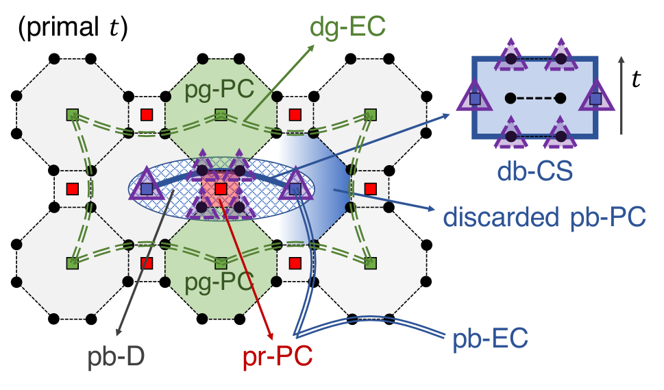
We now investigate the effects of a pc-D $d$ to the nearby PCs. First, all primal PCs whose supports contain any defect qubit no longer survive, while dual PCs are unaffected. Such incompatible PCs may be multiplied with each others to form larger compatible stabilizers, as shown in Fig. 18 where two pg-PCs and a pr-PC are merged. Like normal PCs, these merged PCs also can detect errors, although decoding errors from PCs may get more ambiguous. Some PCs for which such multiplication is impossible have no choice but to be discarded, as the pb-PC in Fig. 18. As a consequence, a pc-EC ending at $d$ is not detected by any PC near $d$.

A pc-D may make some dual CSs survive additionally. The dc-CS $S_{\textup{{CS}}}(f)$ for a face $f\in\mathcal{B}_{2}^{\textup{{dc}}}$, where $Q\quantity(\partial f)$ is in the defect as shown in Fig. 18, is compatible, thus can serve as a PC for detecting errors. We call such CSs defect PCs. A notable thing is that they may detect not only errors on vacuum qubits but also $X$ or $Z$-measurement ($M_{Z}$) errors on defect qubits.

We then identify nontrivial undetectable error chains, where “nontrivial” here means that they incur logical errors. Such an error chain is closed or ends at defects with the same primality and color. Considering the identity gate of a primal logical qubit, the shortest error chain inducing an $X_{L}$ error is a pj-EC ending at the three defects, and the shortest one inducing a $Z_{L}$ error is a closed dc-EC surrounding the $\textup{{pc}}^{\prime}\textup{{-D}}$ ($\textup{{c}}^{\prime}\neq\textup{{c}}$), as shown schematically in Fig. 10 and explicitly in Fig. 18. Note that a closed dc-EC penetrating a defect is detected by defect PCs, although not detected by ordinary PCs. The code distance of a logical qubit is defined by the size of the smallest nontrivial undetectable error set, and it increases as the defects get thicker or get farther from each other ⁵⁵ 5 Such an error set may not be an error chain, because errors in defects may also be nontrivial and undetectable. However, since error correction in defects gets more accurate as the defects get thicker, the dependency of the code distance to their thicknesses is still valid. It can be verified that the smallest nontrivial undetectable error set containing only defect qubits completely covers a cross-section of the defect, thus its size is roughly a quadratic function of the circumference of the defect. .

To correct errors in Y-planes, we use hybrid PCs defined with open PCs, which are visualized in Fig. 19(a).

Remark that CQs in Y-planes are measured in the $Y$ basis, thus ordinary PCs whose supports contain those CQs are incompatible with the qubits. Instead of them, we use hybrid PCs whose $Y$-supports are on the Y-planes, as shown in Fig. 19(b). Error correction in the Y-planes is done with a set of hybrid PCs covering the entire Y-planes.

We now calculate and compare the resource overheads of MBQC via RTCSs or CCCSs. For each case, we consider a periodic hexagonal arrangement of parallel timelike primal defects, where primal logical qubits with the code distances of $d$ are compactly packed in the space. In other words, the intervals of the arrangement are determined to minimize the number of physical qubits per logical qubit while keeping all the possible nontrivial undetectable error chains to contain $d$ or more qubits. We present such arrangements of defects in Appendix B.

Table 3 shows the calculated numbers of physical qubits ($n$) and cz gates ($N_{\mathrm{\textsc{cz}}}$) per layer in terms of $d$ and the number of logical qubits ($k$), considering the optimal hexagonal arrangements. It is worth noticing that MBQC via CCCSs is definitely more resource-efficient than MBQC via RTCSs; $n/k$ is about 1.7–1.8 times smaller for CCCSs than for RTCSs. Note that the compact packing of logical qubits may be unrealistic; extra spaces may be needed for implementing logical gates except the identity gate.

We numerically calculate and compare error thresholds of MBQC via RTCSs and CCCSs.

References

- Galindo and Martín-Delgado (2002) A. Galindo and M. A. Martín-Delgado, Information and computation: Classical and quantum aspects, Rev. Mod. Phys. 74, 347 (2002).
- Nielsen and Chuang (2010) M. A. Nielsen and I. L. Chuang, Quantum Computation and Quantum Information (Cambridge University Press, 2010).
- Shor (1995) P. W. Shor, Scheme for reducing decoherence in quantum computer memory, Phys. Rev. A 52, R2493 (1995).
- Bennett et al. (1996) C. H. Bennett, D. P. DiVincenzo, J. A. Smolin, and W. K. Wootters, Mixed-state entanglement and quantum error correction, Phys. Rev. A 54, 3824 (1996).
- Laflamme et al. (1996) R. Laflamme, C. Miquel, J. P. Paz, and W. H. Zurek, Perfect quantum error correcting code, Phys. Rev. Lett. 77, 198 (1996).
- Calderbank and Shor (1996) A. R. Calderbank and P. W. Shor, Good quantum error-correcting codes exist, Phys. Rev. A 54, 1098 (1996).
- Steane (1996) A. Steane, Multiple-particle interference and quantum error correction, P. Roy. Soc. Lond. A Mat. 452, 2551 (1996).
- Bombín (2013) H. Bombín, Topological codes, in Quantum Error Correction, edited by D. A. Lidar and T. A. Brun (Cambridge, 2013) Chap. 19, pp. 455–481.
- Cory et al. (1998) D. G. Cory, M. D. Price, W. Maas, E. Knill, R. Laflamme, W. H. Zurek, T. F. Havel, and S. S. Somaroo, Experimental quantum error correction, Phys. Rev. Lett. 81, 2152 (1998).
- Chiaverini et al. (2004) J. Chiaverini, D. Leibfried, T. Schaetz, M. D. Barrett, R. B. Blakestad, J. Britton, W. M. Itano, J. D. Jost, E. Knill, C. Langer, R. Ozeri, and D. J. Wineland, Realization of quantum error correction, Nature 432, 602 (2004).
- Schindler et al. (2011) P. Schindler, J. T. Barreiro, T. Monz, V. Nebendahl, D. Nigg, M. Chwalla, M. Hennrich, and R. Blatt, Experimental repetitive quantum error correction, Science 332, 1059 (2011).
- Reed et al. (2012) M. D. Reed, L. DiCarlo, S. E. Nigg, L. Sun, L. Frunzio, S. M. Girvin, and R. J. Schoelkopf, Realization of three-qubit quantum error correction with superconducting circuits, Nature 482, 382 (2012).
- Nigg et al. (2014) D. Nigg, M. Müller, E. A. Martinez, P. Schindler, M. Hennrich, T. Monz, M. A. Martin-Delgado, and R. Blatt, Quantum computations on a topologically encoded qubit, Science 345, 302 (2014).
- Córcoles et al. (2015) A. D. Córcoles, E. Magesan, S. J. Srinivasan, A. W. Cross, M. Steffen, J. M. Gambetta, and J. M. Chow, Demonstration of a quantum error detection code using a square lattice of four superconducting qubits, Nat. Commun. 6, 1 (2015).
- Kelly et al. (2015) J. Kelly, R. Barends, A. G. Fowler, A. Megrant, E. Jeffrey, T. C. White, D. Sank, J. Y. Mutus, B. Campbell, Y. Chen, B. Chiaro, A. Dunsworth, I.-C. Hoi, C. Neill, P. J. J. O’Malley, C. Quintana, P. Roushan, A. Vainsencher, J. Wenner, A. N. Cleland, and J. M. Martinis, State preservation by repetitive error detection in a superconducting quantum circuit, Nature 519, 66 (2015).
- Ofek et al. (2016) N. Ofek, A. Petrenko, R. Heeres, P. Reinhold, Z. Leghtas, B. Vlastakis, Y. Liu, L. Frunzio, S. M. Girvin, L. Jiang, M. Mirrahimi, M. H. Devoret, and R. J. Schoelkopf, Extending the lifetime of a quantum bit with error correction in superconducting circuits, Nature 536, 441 (2016).
- Andersen et al. (2020) C. K. Andersen, A. Remm, S. Lazar, S. Krinner, N. Lacroix, G. J. Norris, M. Gabureac, C. Eichler, and A. Wallraff, Repeated quantum error detection in a surface code, Nat. Phys. 16, 875 (2020).
- Kitaev (1997) A. Y. Kitaev, Quantum computations: algorithms and error correction, Russ. Math. Surv. 52, 1191 (1997).
- Bravyi and Kitaev (1998) S. B. Bravyi and A. Y. Kitaev, Quantum codes on a lattice with boundary, arXiv preprint quant-ph/9811052 (1998).
- Dennis et al. (2002) E. Dennis, A. Kitaev, A. Landahl, and J. Preskill, Topological quantum memory, J. Math. Phys. 43, 4452 (2002).
- Kitaev (2003) A. Y. Kitaev, Fault-tolerant quantum computation by anyons, Ann. Phys. 303, 2 (2003).
- Fowler et al. (2009) A. G. Fowler, A. M. Stephens, and P. Groszkowski, High-threshold universal quantum computation on the surface code, Phys. Rev. A 80, 052312 (2009).
- Bombin and Martin-Delgado (2009) H. Bombin and M. A. Martin-Delgado, Quantum measurements and gates by code deformation, J. Phys. A: Math. Theor. 42, 095302 (2009).
- Fowler et al. (2012a) A. G. Fowler, M. Mariantoni, J. M. Martinis, and A. N. Cleland, Surface codes: Towards practical large-scale quantum computation, Phys. Rev. A 86, 032324 (2012a).
- Terhal (2015) B. M. Terhal, Quantum error correction for quantum memories, Rev. Mod. Phys. 87, 307 (2015).
- Bombin and Martin-Delgado (2006) H. Bombin and M. A. Martin-Delgado, Topological quantum distillation, Phys. Rev. Lett. 97, 180501 (2006).
- Fowler (2011) A. G. Fowler, Two-dimensional color-code quantum computation, Phys. Rev. A 83, 042310 (2011).
- Kesselring et al. (2018) M. S. Kesselring, F. Pastawski, J. Eisert, and B. J. Brown, The boundaries and twist defects of the color code and their applications to topological quantum computation, Quantum 2, 101 (2018).
- (29) That a logical gate is transversal means that can be expressed as such that a unitary operator acts only on the th physical qubit for each logical qubit for all ’s. For example, if for code where is the operator on the th physical qubit, is transversal. Specific 2D color codes implement the logical Hadamard gate by the combination of the Hadamard gate on every physical qubit, and similarly for the logical phase gate Bombin and Martin-Delgado 2006; Fowler 2011.
- Bombin and Martin-Delgado (2007a) H. Bombin and M. A. Martin-Delgado, Topological computation without braiding, Phys. Rev. Lett. 98, 160502 (2007a).
- Bombin and Martin-Delgado (2007b) H. Bombin and M. A. Martin-Delgado, Exact topological quantum order in and beyond: Branyons and brane-net condensates, Phys. Rev. B 75, 075103 (2007b).
- Bombín (2015) H. Bombín, Gauge color codes: optimal transversal gates and gauge fixing in topological stabilizer codes, New J. Phys. 17, 083002 (2015).
- Kubica and Beverland (2015) A. Kubica and M. E. Beverland, Universal transversal gates with color codes: A simplified approach, Phys. Rev. A 91, 032330 (2015).
- Watson et al. (2015) F. H. E. Watson, E. T. Campbell, H. Anwar, and D. E. Browne, Qudit color codes and gauge color codes in all spatial dimensions, Phys. Rev. A 92, 022312 (2015).
- Kubica et al. (2018) A. Kubica, M. E. Beverland, F. Brandão, J. Preskill, and K. M. Svore, Three-dimensional color code thresholds via statistical-mechanical mapping, Phys. Rev. Lett. 120, 180501 (2018).
- Bombin (2018a) H. Bombin, 2d quantum computation with 3d topological codes, arXiv preprint arXiv:1810.09571 (2018a).
- Bombin (2018b) H. Bombin, Transversal gates and error propagation in 3d topological codes, arXiv preprint arXiv:1810.09575 (2018b).
- Bravyi and Kitaev (2005) S. Bravyi and A. Kitaev, Universal quantum computation with ideal clifford gates and noisy ancillas, Phys. Rev. A 71, 022316 (2005).
- Jones (2013) C. Jones, Multilevel distillation of magic states for quantum computing, Phys. Rev. A 87, 042305 (2013).
- Raussendorf et al. (2007) R. Raussendorf, J. Harrington, and K. Goyal, Topological fault-tolerance in cluster state quantum computation, New J. Phys. 9, 199 (2007).
- Raussendorf and Briegel (2001) R. Raussendorf and H. J. Briegel, A one-way quantum computer, Phys. Rev. Lett. 86, 5188 (2001).
- Raussendorf et al. (2003) R. Raussendorf, D. E. Browne, and H. J. Briegel, Measurement-based quantum computation on cluster states, Phys. Rev. A 68, 022312 (2003).
- Raussendorf et al. (2006) R. Raussendorf, J. Harrington, and K. Goyal, A fault-tolerant one-way quantum computer, Ann. Phys. 321, 2242 (2006).
- Raussendorf and Harrington (2007) R. Raussendorf and J. Harrington, Fault-tolerant quantum computation with high threshold in two dimensions, Phys. Rev. Lett. 98, 190504 (2007).
- Fowler and Goyal (2009) A. G. Fowler and K. Goyal, Topological cluster state quantum computing, Quantum Info. Comput. 9, 721–738 (2009).
- Barrett and Stace (2010) S. D. Barrett and T. M. Stace, Fault tolerant quantum computation with very high threshold for loss errors, Phys. Rev. Lett. 105, 200502 (2010).
- Whiteside and Fowler (2014) A. C. Whiteside and A. G. Fowler, Upper bound for loss in practical topological-cluster-state quantum computing, Phys. Rev. A 90, 052316 (2014).
- Li et al. (2010) Y. Li, S. D. Barrett, T. M. Stace, and S. C. Benjamin, Fault tolerant quantum computation with nondeterministic gates, Phys. Rev. Lett. 105, 250502 (2010).
- Nielsen (2004) M. A. Nielsen, Optical quantum computation using cluster states, Phys. Rev. Lett. 93, 040503 (2004).
- Dawson et al. (2006) C. M. Dawson, H. L. Haselgrove, and M. A. Nielsen, Noise thresholds for optical cluster-state quantum computation, Phys. Rev. A 73, 052306 (2006).
- Menicucci et al. (2006) N. C. Menicucci, P. van Loock, M. Gu, C. Weedbrook, T. C. Ralph, and M. A. Nielsen, Universal quantum computation with continuous-variable cluster states, Phys. Rev. Lett. 97, 110501 (2006).
- Devitt et al. (2009) S. J. Devitt, A. G. Fowler, A. M. Stephens, A. D. Greentree, L. C. L. Hollenberg, W. J. Munro, and K. Nemoto, Architectural design for a topological cluster state quantum computer, New J. Phys. 11, 083032 (2009).
- Herrera-Martí et al. (2010) D. A. Herrera-Martí, A. G. Fowler, D. Jennings, and T. Rudolph, Photonic implementation for the topological cluster-state quantum computer, Phys. Rev. A 82, 032332 (2010).
- Fujii and Tokunaga (2010) K. Fujii and Y. Tokunaga, Fault-tolerant topological one-way quantum computation with probabilistic two-qubit gates, Phys. Rev. Lett. 105, 250503 (2010).
- Myers and Ralph (2011) C. R. Myers and T. C. Ralph, Coherent state topological cluster state production, New J. Phys. 13, 115015 (2011).
- Yao et al. (2012) X.-C. Yao, T.-X. Wang, H.-Z. Chen, W.-B. Gao, A. G. Fowler, R. Raussendorf, Z.-B. Chen, N.-L. Liu, C.-Y. Lu, Y.-J. Deng, Y.-A. Chen, and J.-W. Pan, Experimental demonstration of topological error correction, Nature 482, 489 (2012).
- Gimeno-Segovia et al. (2015) M. Gimeno-Segovia, P. Shadbolt, D. E. Browne, and T. Rudolph, From three-photon greenberger-horne-zeilinger states to ballistic universal quantum computation, Phys. Rev. Lett. 115, 020502 (2015).
- Li et al. (2015) Y. Li, P. C. Humphreys, G. J. Mendoza, and S. C. Benjamin, Resource costs for fault-tolerant linear optical quantum computing, Phys. Rev. X 5, 041007 (2015).
- Omkar et al. (2020) S. Omkar, Y. S. Teo, and H. Jeong, Resource-efficient topological fault-tolerant quantum computation with hybrid entanglement of light, Phys. Rev. Lett. 125, 060501 (2020).
- Bolt et al. (2016) A. Bolt, G. Duclos-Cianci, D. Poulin, and T. M. Stace, Foliated quantum error-correcting codes, Phys. Rev. Lett. 117, 070501 (2016).
- Bolt et al. (2018) A. Bolt, D. Poulin, and T. M. Stace, Decoding schemes for foliated sparse quantum error-correcting codes, Phys. Rev. A 98, 062302 (2018).
- Brown and Roberts (2020) B. J. Brown and S. Roberts, Universal fault-tolerant measurement-based quantum computation, Phys. Rev. Research 2, 033305 (2020).
- (63) The support of an operator , written as , is the set of qubits on which applies non-trivially.
- (64) If this is the case, the interior qubits of the CS correspond to spacelike faces in , which are s () according to Table 1. They are surely not be in the pc-D. Otherwise, the pc′-CS and defect share at least one qubit if they overlap.
- (65) The boundary qubits of a dc-CS correspond to edges in , which are pcAQs or pcLs.
- (66) Such an error set may not be an error chain, because errors in defects may also be nontrivial and undetectable. However, since error correction in defects gets more accurate as the defects get thicker, the dependency of the code distance to their thicknesses is still valid. It can be verified that the smallest nontrivial undetectable error set containing only defect qubits completely covers a cross-section of the defect, thus its size is roughly a quadratic function of the circumference of the defect.
- Edmonds (1965a) J. Edmonds, Paths, trees, and flowers, Can. J. Math. 17, 449 (1965a).
- Edmonds (1965b) J. Edmonds, Maximum matching and a polyhedron with 0, 1-vertices, J. Res. Nat. Bur. Stand. B 69, 55 (1965b).
- Fowler (2015) A. G. Fowler, Minimum weight perfect matching of fault-tolerant topological quantum error correction in average o(1) parallel time, Quantum Info. Comput. 15, 145–158 (2015).
- Kolmogorov (2009) V. Kolmogorov, Blossom v: a new implementation of a minimum cost perfect matching algorithm, Math. Program. Comput. 1, 43 (2009).
- Litinski (2019) D. Litinski, Magic State Distillation: Not as Costly as You Think, Quantum 3, 205 (2019).
- Chamberland and Noh (2020) C. Chamberland and K. Noh, Very low overhead fault-tolerant magic state preparation using redundant ancilla encoding and flag qubits, npj Quant. Inf. 6, 1 (2020).
- Roberts and Williamson (2020) S. Roberts and D. J. Williamson, 3-fermion topological quantum computation, arXiv preprint arXiv:2011.04693 (2020).
- Fowler et al. (2012b) A. G. Fowler, A. C. Whiteside, A. L. McInnes, and A. Rabbani, Topological code autotune, Phys. Rev. X 2, 041003 (2012b).