Cross-replication Reliability -
An Empirical Approach to Interpreting Inter-rater Reliability
ACL 2021 Main Conference
Abstract
When collecting annotations and labeled data from humans, a standard practice is to use inter-rater reliability (IRR) as a measure of data goodness Hallgren 2012. Metrics such as Krippendorff’s alpha or Cohen’s kappa are typically required to be above a threshold of 0.6 Landis and Koch 1977. These absolute thresholds are unreasonable for crowdsourced data from annotators with high cultural and training variances, especially on subjective topics. We present a new alternative to interpreting IRR that is more empirical and contextualized. It is based upon benchmarking IRR against baseline measures in a replication, one of which is a novel cross-replication reliability (xRR) measure based on Cohen’s (1960) kappa. We call this approach the xRR framework. We opensource a replication dataset of 4 million human judgements of facial expressions and analyze it with the proposed framework. We argue this framework can be used to measure the quality of crowdsourced datasets.
1 Introduction
Much content analysis and linguistics research is based on data generated by human beings (henceforth, annotators or raters) asked to make some kind of judgment. These judgments involve systematic interpretation of textual, visual, or audible matter (e.g. newspaper articles, television programs, advertisements, public speeches, and other multimodal data). When relying on human observers, researchers must worry about the quality of the data — specifically, their reliability Krippendorff 2004. Are the annotations collected reproducible, or are they the result of human idiosyncrasies?
Respectable scholarly journals typically require reporting quantitative evidence for the inter-rater reliability (IRR) of the data Hallgren 2012. Cohen’s kappa Cohen 1960 or Krippendorff’s alpha Hayes and Krippendorff 2007 is expected to be above a certain threshold to be worthy of publication, typically 0.6 Landis and Koch 1977. Similar IRR requirements for human annotations data have been followed across many fields. In this paper we refer to this absolute interpretation of IRR as the Landis-Koch approach (Fig. 1).

This approach has been foundational in guiding the development of widely used and shared datasets and resources. Meanwhile, the landscape of human annotations collection has witnessed a tectonic shift in recent years. Driven by the data-hungry success of machine learning LeCun et al. 2015; Schaekermann et al. 2020, there has been an explosive growth in the use of crowdsourcing for building datasets and benchmarks Snow et al. 2008; Kochhar et al. 2010. We identify three paradigm shifts in the scope of and methodologies for data collection that make the Landis-Koch approach not as useful in today’s settings.
A rise in annotator diversity
In the pre-crowdsourcing era lab settings, data were typically annotated by two graduate students following detailed guidelines and working with balanced corpora. Over the past two decades, however, the bulk of data are annotated by crowd workers with high cultural and training variances.
A rise in task diversity
There has been an increasing amount of subjective tasks with genuine ambiguity: judging toxicity of online discussions Aroyo et al. 2019, in which the IRR values range between 0.2 and 0.4; judging emotions expressed by faces Cowen and Keltner 2017, in which more than 80% of the IRR values are below 0.6; and A/B testing of user satisfaction or preference evaluations Kohavi and Longbotham 2017, where IRR values are typically between 0.3 and 0.5.
A rise in imbalanced datasets
Datasets are no longer balanced intentionally. Many high-stakes human judgements concern rare events with substantial tail risks: event security, disease diagnostics, financial fraud, etc. In all of these cases, a single rare event can be the source of considerable cost. High class imbalance has led to many complaints of IRR interpretability Byrt et al. 1993; Feinstein and Cicchetti 1990; Cicchetti and Feinstein 1990.
Each of these changes individually has a profound impact on data reliability. Together, they have caused a shift from data-from-the-lab to data-from-the-wild, for which the Landis-Koch approach to interpreting IRR is admittedly too rigid and too stringent. Meanwhile, we have seen a drop in the reliance on reliability. Machine learning, crowdsourcing, and data research papers and tracks have abandoned the use and reporting of IRR for human labeled data, despite calls for it Paritosh 2012. The most cited recent datasets and benchmarks used by the community such as SQuAD Rajpurkar et al. 2016, ImageNet Deng et al. 2009, Freebase Bollacker et al. 2008, have never reported IRR values. This would have been unthinkable twenty years ago. More importantly, this is happening against the backdrop of a reproducibility crisis in artificial intelligence Hutson 2018.
With the decline of the usage of IRR, we have seen a rise of ad hoc, misguided quality metrics that took its place, including 1) agreement-%, 2) accuracy relative to consensus, 3) accuracy relative to “ground truth.” This is dangerous, as IRR is still our best bet for ensuring data reliability. How can we ensure its continued importance in this new era of data collection?
This paper is an attempt to address this problem by proposing an empirical alternative to interpreting IRR. Instead of relying on an absolute scale, we benchmark an experiment’s IRR against two baseline measures, to be found in a replication. Replication here is defined as re-annotating the same set of items with a slight change in the experimental setup, e.g., annotator population, annotation guidelines, etc. By fixing the underlying corpus, we can ensure the baseline measures are sensitive to the experiment on hand. The first baseline measure is the annotator reliability in the replication. The second measure is the annotator reliability between the replications. In Section 3, we present a novel way of measuring this. We call it cross-kappa (). It is an extension of Cohen’s (1960) kappa and is designed to measure annotator agreement between two replications in a chance-corrected manner.
We present in Appendix A the International Replication (IRep) dataset,11 1 https://github.com/google-research-datasets/replication-dataset a large-scale crowdsourced dataset of four million judgements of human facial expressions in videos. The dataset consists of three replications in Mexico City, Budapest, and Kuala Lumpur.22 2 On this task, raters received average hourly wages of $12, $20, and $14 USD in Mexico City, Budapest, and Kuala Lumpur respectively. See Appendix A for annotation setup. Our analysis in Section 4 shows this empirical approach enables meaningful interpretation of IRR. In Section 5, we argue xRR is a sensible way of measuring the goodness of crowdsourced datasets, where high reliability is unattainable. While we only illustrate comparing annotator populations in this paper, the methodology behind the xRR framework is general and can apply to similarly replicated datasets, e.g., via change of annotation guidelines.
2 Related Work
To position our research, we present a brief summary of the literature in two areas: metrics for measuring annotator agreement and their shortcomings (Section 2.1), comparing replications of an experiment (Section 2.2).
2.1 Annotator Agreement
Artstein and Poesio 2008 present a comprehensive survey of the literature on IRR metrics used in linguistics. Popping 1988 compare an astounding 43 measures for nominal data (mostly applicable to reliability of data generated by only two observers). Since then, Cohen’s (1960) kappa and its variants Carletta et al. 1997; Cohen 1968 have become the de facto standard for measuring agreement in computational linguistics.
One of the strongest criticisms of kappa is its lack of interpretability when facing class imbalance. This problem is known as the kappa paradox Feinstein and Cicchetti 1990; Byrt et al. 1993; Warrens 2010, or the ‘base rates’ problem Uebersax 1987. Bruckner and Yoder 2006 show class imbalance imposes practical limits on kappa and suggest one to interpret kappa in relation to the class imbalance of the underyling data. Others have proposed measures that are more robust against class imbalance Gwet 2008; Spitznagel and Helzer 1985; Stewart and Rey 1988. Pontius Jr and Millones 2011 even suggest abandoning the use of kappa altogether.
2.2 Agreement Between Replications
Replications are often being compared, but it is done at the level of per-item mean scores. Cowen and Keltner 2017 measure the correlation between the mean scores of two geographical rater pools. They use Spearman’s (1904) correction for attenuation (discussed later in this paper) with split-half reliability. Snow et al. 2008 measure the Pearson correlations between the score of a single expert and the mean score of a group of non-experts, and vice versa. In this comparison the authors do not correct for correlation attenuation, hence the reported correlations may be strongly biased. Bias aside, correlation is not suitable for tasks with non-interval data or task with missing data. In this paper, we propose a general methodology for measuring rater agreement between replications with the same kind of generality, flexibility, and ease of use as IRR.
3 Cross-replication Reliability (xRR)
Data reliability can be assessed when a set of items are annotated multiple times. When this is done by a single rater, intra-rater reliability assesses a person’s agreement with oneself. When this is done by two or more raters, inter-rater reliability (IRR) assesses the agreement between raters in an experiment. We propose to extend IRR to measure a similar notion of rater-rater agreement, but where the raters are taken from two different experiments. We call it cross-replication reliability (xRR). These replications can be a result of re-labeling the same items with a different rater pool, annotation template, or on a different platform, etc.
We begin with a general definition of Cohen’s (1960) kappa. We extend it to cross-kappa () to measure cross-replication reliability. We then use this foundation to define normalized to measure similarity between two replications.
3.1 Kappa and Its Generalizations
The class of IRR measures is quite diverse, covering many different experimental scenarios, e.g., different numbers of raters, rating scales, agreement definitions, assumptions about rater interchangeability, etc. Out of all such coefficients, Cohen’s (1960) kappa has a distinct property that makes it most suitable for the task on hand. Unlike Scott’s pi Scott 1955, Fleiss’s kappa Fleiss 1971, Krippendorf’s alpha Krippendorff 2004, and many others, Cohen’s (1960) kappa allows for two different marginal distributions. This stems from Cohen’s belief that two raters do not necessarily share the same marginal distribution, hence they should not be treated interchangeably. When we compare replications, e.g., two rater populations, we are deliberately changing some underlying conditions of the experiment, hence it is safer to assume the marginal distributions will not be the same. Within either replication, however, we rely on the rater interchangeability assumption. We think this more accurately reflects the current practice in crowdsourcing, where each rater contributes a limited number of responses in an experiment, and hence raters are operationally interchangeable.
Cohen’s (1960) kappa was invented to compare two raters classifying items into a fixed number of categories. Since its publication, it has been generalized to accommodate multiple raters Light 1971; Berry and Mielke Jr 1988, and to cover different types of annotation scales: ordinal Cohen 1968, interval Berry and Mielke Jr 1988; Janson and Olsson 2001, multivariate Berry and Mielke Jr 1988, and any arbitrary distance function Artstein and Poesio 2008. In this paper we focus on Janson and Olsson’s (2001) generalization, which the authors denote with the lowercase Greek letter iota (). It extends kappa to accommodate interval data with multiple raters, and is expressed in terms of pairwise disagreement:
| (1) |
in this formula represents the observed portion of disagreement and is defined as:
| (2) |
where is the number of items, the number of annotators, the item index, and the annotator indexes; is the sum over all and such that . is a pairwise disagreement defined as:
| (3) |
for interval data, and
| (4) |
for categorical data. Note we are dropping Janson and Olsson’s multivariate reference in and focusing on the univariate case. in the denominator represents the expected portion of disagreement and is defined as:
| (5) |
Janson and Olsson’s expression in Eq. 1 is based on Berry and Mielke Jr 1988. While the latter use absolute distance for interval data, the former use squared distance instead. We follow Janson and Olsson’s approach because squared distance leads to desirable properties and familiar interpretation of coefficients Fleiss and Cohen 1973; Krippendorff 1970. Squared distance is also used in alpha Krippendorff 2004. Berry and Mielke Jr 1988 show if and the scale is categorical, in Eq. 1 reduces to Cohen’s (1960) kappa. For other rating scales such as ratio, rank, readers should refer to Krippendorff 2004 for additional distance functions. The equations for and are unaffected by the choice of .
3.2 Definition of
Here we present as a novel reliability coefficient for measuring the rater agreement between two replications. In Janson and Olsson’s generalized kappa above, the disagreement is measured within pairs of annotations taken from the same experiment. In order to extend it to measure cross-replication agreement, we construct annotation pairs such that the two annotations are taken from different replications. We do not consider annotation pairs from the same replication. We define cross-kappa, , as a reliability coefficient between replications and :
| (6) |
where
| (7) |
and
| (8) |
where and denote annotations from replications and respectively, is the number of items, and the numbers of annotations per item in replications and respectively. In this definition, the observed disagreement is obtained by averaging disagreement observed in pairs of annotations, where each pair contains two annotations on the same item taken from two different replications. Expected disagreement is obtained by averaging over all possible cross-replication annotation pairs. When each replication has only 1 annotation per item, and the data is categorical, it is easy to show reduces to Cohen’s (1960) kappa.
is a kappa-like measure, and will have properties similar to kappa’s. is bounded between 0 and 1 in theory, though in practice it may be slightly negative for small sample sizes. means there is no discernible agreement between raters from two replications, beyond what would be expected by chance. means all raters between two replications are in perfect agreement with each other, which also implies perfect agreement within either replication.
3.3 with Missing Data
As presented, the two replications can have different numbers of annotations per item. However, within either replication, the number of annotations per item is assumed to be fixed. We recognize this may not always be the case. In practice, items within an experiment can receive varying numbers of annotations (i.e., missing data). We now show how to calculate with missing data.
When computing IRR with missing data, weights can be used to account for varying numbers of annotations within each item. Janson and Olsson 2004 propose a weighting scheme for iota in Eq. 1. Instead, we follow the tradition of Krippendorff 2004 in weighting each annotation equally in computing and . That amounts to the following scheme. In , we first normalize within each item, then we take a weighted average over all items, with weights proportional to the combined numbers of annotations per item. In , no weighting is required.
Since and can now vary from item to item, we index them using and to denote that they are functions of the underlying items. We rewrite and as:
| (9) |
and
| (10) |
with
| (11) |
where is the total number of annotations in replications , the number annotations on item in replication , (on item in replication ); and similarly for , , and with respect to replication . and in Eq. 9 and 10 are inner summations, where and are indexes from the outer summations. Without missing data, for all , and for all , then , , reducing Eq. 9 and 10 to Eq. 7 and 8.
3.4 Normalization of
xRR is modeled closely after IRR in order to serve as its baseline. As IRR measures the agreement between raters, so does xRR. In other words, is really a measure of rater agreement, not a measure of experimental similarity per se. This distinction is important. If we want to measure how well we replicate an experiment, we need to measure its disagreement with the replication in relationship to their own internal disagreements. The departure between inter-experiment and intra-experiment disagreements is important in measuring experimental similarity.
This calls for a normalization that considers in relation to IRR. First, we take inspirations from Spearman’s correction for attenuation Spearman 1904:
| (12) |
where is the observed Pearson product-moment correlation between and (variables observed with measurement errors), is an estimate of their true, unobserved correlation (in the absence of measurement errors), and and are the reliabilities of and respectively. Eq. 12 is Spearman’s attempt to correct for the negative bias in caused by the observation errors in and .33 3 Spearman relied on the assumption that the errors are uncorrelated with each other and with and .
Eq. 12 is relevant here because of the close connection between Cohen’s (1960) kappa and the Pearson correlation, . In the dichotomous case, if the two marginal distributions are the same, Cohen’s (1960) kappa is equivalent to the Pearson correlation Cohen 1960; Cohen 1968. In the multi-category case, Cohen 1968 generalizes this equivalence to weighted kappa, under the conditions of equal marginals and a specific quadratic weighting scheme.
Based on this strong connection, we propose replacing in Eq. 12 with and define normalized as:
| (13) |
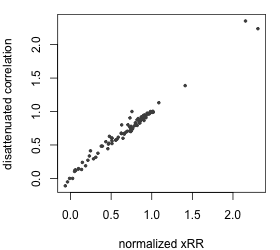
Defined this way, one would expect normalized to behave like . That is indeed the case. When we apply both measures to the IRep dataset, we obtain a Pearson correlation of 0.99 between them (see Section 4.5). This leads to two insights. First, we can interpret normalized like a disattenuated correlation, (see Muchinsky 1996 for a rigorous interpretation). Second, normalized approximates the true correlation between two experiments’ item-level mean scores.
Despite their affinity, is not a substitute for normalized for measuring experimental similarity. Normalized is more general as it can accommodate non-interval scales and missing data.
3.5 Connection between xRR and IRR
By connecting normalized to , we can also learn a lot about itself. To the extent that normalized approximates , we can rewrite Eq. 13 as:
| (14) |
This formulation shows behaves like a product of and the geometric mean of the two IRRs. This has important consequences, as we can deduce the following. 1) Holding constant the mean scores, and hence , the lower the IRRs, the lower the . Intra-experiment disagreement inflates inter-experiment disagreement. 2) In theory ,44 4 Spearman’s correction can occasionally produce a correlation above 1.0 Muchinsky 1996. hence is capped by the greater of the two IRRs. I.e., Intra-experiment agreement presents a ceiling to inter-experiment agreement. 3) If and are identically distributed, e.g., in a perfect replication, and . Thus, when a low reliability experiment is replicated perfectly, will be as low, whereas normalized will be 1. This explains why normalized is more suitable for measuring experimental similarity.
In this section, we propose as a measure of rater agreement between two replications, and normalized is as an experimental similarity metric. In the next section, we apply them in conjunction with IRR to illustrate how we can gain deeper insights into experiment reliabilities by triangulating these measures.
4 Applying xRR to the IRep Dataset
As a standalone measure, IRR captures the reliability of an experiment by encapsulating many of its facets: class imbalance, item difficulty, guideline clarity, rater qualification, task ambiguity, etc. As such, it is difficult to compare the IRR of different experiments, or to interpret their individual values, because IRR is tangled with all the aforementioned design parameters. For example, we cannot attribute a low IRR to rater qualification without first isolating other design parameters. This is the problem we try to solve with xRR by contextualizing IRR with meaningful baselines via a replication. We will demonstrate this by applying this technique to the IRep Dataset (Appendix A). We focus on a subset of 5 emotions for illustration purposes, with the rest of the reliability values provided in Appendix B. In our analysis, IRR is measured with Cohen’s (1960) kappa and xRR with . We will refer to them interchangeably.
4.1 IRR Variability Across Emotions
First we illustrate in Fig. 2 that different emotions within the same city can have very different IRR. For instance, the labels awe and love in Mexico City have an IRR of 0.1208 and 0.597 respectively (Table 1). Awe and love are completely different emotions with different levels of class imbalance and ambiguity, and without controlling for these differences, the gap in their reliabilities is not unexpected. That is exactly the problem about comparing IRRs – such comparisons are not meaningful. We need something directly comparable to awe in order to interpret its low IRR. If we do not compare emotions, and just consider awe using the Landis-Koch scale, that would not be helpful either. We would not be able to tell if its low IRR is a result of poor guidelines, general ambiguity in emotion detection, or ambiguity specific to awe. It’s more meaningful to compare replications of awe itself.


4.2 IRR Variability Across Replications
While the aforementioned variation in IRR between emotions is expected, IRR of the same emotion can vary greatly between replications as well. Fig. 3 shows two contrasting examples. On the one hand, the IRR of love is consistent across replications. On the other hand, the IRR of contemplation varies a lot. We know the IRR variation in contemplation is strictly attributed to rater pool differences because the samples, platforms and annotation templates are the same across experiments. Such variation in IRR will be missed entirely by sampling based approaches for error-bars (e.g. standard error, bootstrap), which assume a fixed rater population.

4.3 Cross-replication Rater Agreement
As shown, replication can facilitate comparisons of IRR by producing meaningful baselines. However, IRR is an internal property of a dataset, it does not allow us to compare two datasets directly. To that end, we can apply to quantify the rater agreement between two datasets, as IRR quantifies the rater agreement within a dataset. Interestingly, not only is useful for comparing two datasets, but it also serves as another baseline for interpreting their IRRs.
IRR is a step toward ensuring reproducibility, so naturally we wonder how much of the observed IRR is tied to the specific experiment and how much of it generalizes? This is of particular concern when raters are sampled in a clustered manner, e.g., crowd workers from the same geographical region, grad students sharing the same office. We rarely make sure raters are diverse and representative of the larger population. High IRR can be the result of a homogeneous rater group, limiting the generality of the results. In the context of the IRep dataset, that two cities having similar IRRs does not imply their raters agree with each other at a comparable level, or at all. We will demonstrate this with two contrasting examples.


Mexico City and Budapest both have a moderate IRR for sadness, 0.5147 and 0.5175 respectively, and their is nearly the same at 0.4709 (Fig. 4). This gives us confidence that the high IRR of sadness generalizes beyond the specific rater pools. In contrast, on contentment Mexico City and Kuala Lumpur have comparable levels of IRR, 0.4494 and 0.6363 respectively, but their is an abysmal -0.0344 55 5 Negative xRR value due to estimation error. (Fig. 5). In other words, the rater agreement on contentment is limited to within-pool observations only. This serves as an important reminder that IRR is a property of a specific experimental setup and may or may not generalize beyond that. allows us to ensure the internal agreement has external validity.
4.4 Replication Similarity
is a step towards comparing two replications, but it is not a good standalone measure of replication similarity. To do that, we must also account for both replications’ internal agreements, e.g., via normalized in Eq. 13. Fig. 6 shows an example. Mexico City and Budapest have a low of 0.0817 on awe. On the surface, this low agreement may seem attributable to differences between the rater pools. However, there is a similarly low IRR in either city: 0.1208 in Mexico City, and 0.117 in Budapest. After accounting for IRR, normalized is much higher at 0.6872 (Table 2), indicating a decent replication similarity between the two cities.


4.5 Connection to
We apply Spearman’s correction for attenuation in Eq. 12 to all 31 emotion labels in 3 replication pairs. The resulting is plotted against the corresponding normalized in Fig. 7. Both measures are strongly correlated with a Pearson correlation of 0.99. This justifies interpreting normalized as a disattenuated correlation like .
5 Measuring the Quality of a Crowdsourced Dataset
The IRep dataset is replicated and is conducive to xRR analysis. However, in practice most datasets are not replicated. Is xRR still useful? We present a specific use case of xRR in this section and argue that it is worth replicating a crowdsourced dataset in order to evaluate its quality.
5.1 Data Target
Given a set of items, it is possible that annotations of the highest attainable quality still fail to meet the Landis-Koch requirements. Task subjectivity and class imbalance together impose a practical limit on kappa Bruckner and Yoder 2006. In these situations, the experimenter can forgo a data collection effort for reliability reasons. Alternatively, the experimenter may believe that data of sufficiently high quality can still have scientific merits, regardless of reliability. If so, what guidance can we use to ensure the highest quality data, especially when collecting data via crowdsourcing? This paper is heavily motivated by this question.
xRR allows us to interpret IRR not on an absolute scale, but against a replication, a reference of sorts. By judging a crowdsourced dataset against a reference, we can decide if its meets a certain quality bar, albeit a relative one. In the IRep dataset, all replications are of equal importance. However, in practice, we can often define a trusted source as our target. This trusted source can consist of linguists, medical experts, calibrated crowd workers, or the experimenters themselves. They should have enough expertise knowledge and an adequate understanding of the task. The critical criterion in choosing a target is its ability to remove common quality concerns such as rater qualification and guideline effectiveness.
5.2 Internal Agreements
By replicating a random subset of a crowdsourced dataset with trusted annotators,66 6 2 or more ratings per item are needed to measure the IRR. one can compare the two IRRs and make sure they are at a similar level. If the crowd IRR is much higher, that may be an indication of collusion, or a set of overly simplistic guidelines that have deviated from the experiment fidelity Sameki et al. 2015. If the crowd IRR is much lower, it may just be a reflection of annotator diversity, or it can mean under-defined guidelines, unequal annotator qualifications, etc. Further investigation is needed to ensure the discrepancy is reasonable and appropriate.
5.3 Mutual Agreement
Suppose the two IRRs are similar, that is not to say that both datasets are similar. Both groups of annotators can have high internal agreement amongst themselves, but the two groups can agree on different sets of items. If our goal is to collect crowdsourced data that closely mirror the target, then we have to measure their mutual agreement, in addition to comparing their internal agreements. Recall from Section 3.5 that if an experiment is replicated perfectly, should be identical to the two IRRs. Or more concisely, normalized should be equal to 1. Thus a high normalized can assure us that the crowdsourced annotators are functioning as an extension of the trusted annotators, based on which we form our expectations.
5.4 Relation to Gold Data
At a glance, this approach seems similar to the common practice of measuring the accuracy of crowdsourced data against the ground truth Resnik et al. 2006; Hripcsak and Wilcox 2002. However, they are actually fundamentally different approaches. is rooted in the reliability literature that does not rely on the existence of a correct answer. The authors argue this is an unrealistic assumption for many crowdsourcing tasks, where the input involves some subjective judgement. Accuracy itself is also a flawed metric for annotations data due to its inability to handle data uncertainty. For instance, when the reliability of the gold data is less than perfect, accuracy can never reach 1.0. Furthermore, accuracy is not chance-corrected, so it tends to inflate with class imbalance.
5.5 Extending an Existing Dataset
The aforementioned technique can also measure the quality of a dataset extension. The main challenge in extending an existing dataset is to ensure the new data is consistent with the old. The state-of-the-art method in computer vision is frequency matching – ensuring the same proportion of yes/no votes in each image class. Recht et al. 2019 extended ImageNet77 7 http://www.image-net.org/ using this technique, concluding there is a 11% - 14% drop in accuracy across a broad range of models. While frequency matching controls the distribution of some statistics, the impact of the new platform is uncontrolled for. Engstrom et al. 2020 pointed out a bias in this sampling technique. Overall, it is difficult to assess how well we are extending a dataset. To that end, xRR can be of help. A high normalized and a comparable IRR in the new data can give us confidence in the uniformity and continuity in the data collection.
6 Discussion
There has been a tectonic shift in the scope of and methodologies for annotations data collection due to the rise of crowdsourcing and machine learning. In many of these tasks, a high reliability is often difficult to attain, even under favorable circumstances. The rigid Landis-Koch scale has resulted in a decrease in the usage and reporting of IRR in most widely used datasets and benchmarks. Instead of abandoning IRR, we should adapt it to new ways of measuring data quality. The xRR framework presents a first-principled way of doing so. It is a more empirical approach that utilizes a replication as a reference point. It is based on two metrics – for measuring cross-replication rater agreement – and normalized for measuring replication similarity.
We opensource a large-scale replication dataset of facial expression judgements analyzed with the proposed framework. We show this framework can be used to guide our crowdsourcing data collection efforts. This is the beginning of a long line of inquiry. We outline future work and limitations below:
Confidence intervals for
Confidence intervals for and normalized are required for hypothesis testing. Though one can use the block-bootstrap for an empirical estimate, large sample behavior of these metrics needs to be studied.
Sensitivity of with high class-imbalance
The xRR framework sidesteps the effect of class-imbalance by comparing replications on the same item set. Further analysis needs to confirm the sensitivity of metrics in high class-imbalance.
Optimization of computation
Our method requires constructing many pairs of observations: . This may get prohibitively expensive, when the number of items is large. Using algebraic simplification and dynamic programming, this can be made much more efficient.
Alternative normalizations of
We provided one particular normalization technique, but it may not suit all applications. For example, when comparing crowd annotations to expert annotations, one can consider, IRRexpert.
Alternative xRR coefficients
Our proposed xRR coefficient, , is based on Cohen’s (1960) kappa for its assumption about rater non-interchangeability. It may be useful to consider Krippendorff’s alpha and other agreement statistics as alternatives for other assumptions and statistical characteristics.
We hope this paper and dataset will spark research on these questions and increase reporting of reliability measures for human annotated data.
Acknowledgments
We like to thank Gautam Prasad and Alan Cowen for their work on collecting and sharing the IRep dataset and opensourcing it.
References
- Aroyo et al. (2019) Lora Aroyo, Lucas Dixon, Nithum Thain, Olivia Redfield, and Rachel Rosen. 2019. Crowdsourcing subjective tasks: The case study of understanding toxicity in online discussions. In Companion Proceedings of The 2019 World Wide Web Conference, WWW ’19, page 1100–1105, New York, NY, USA. Association for Computing Machinery.
- Artstein and Poesio (2008) Ron Artstein and Massimo Poesio. 2008. Inter-coder agreement for computational linguistics. Computational Linguistics, 34(4):555–596.
- Berry and Mielke Jr (1988) Kenneth J. Berry and Paul W. Mielke Jr. 1988. A generalization of cohen’s kappa agreement measure to interval measurement and multiple raters. Educational and Psychological Measurement, 48(4):921–933.
- Bollacker et al. (2008) Kurt Bollacker, Colin Evans, Praveen Paritosh, Tim Sturge, and Jamie Taylor. 2008. Freebase: A collaboratively created graph database for structuring human knowledge. In Proceedings of the 2008 ACM SIGMOD International Conference on Management of Data, SIGMOD ’08, page 1247–1250, New York, NY, USA. Association for Computing Machinery.
- Bruckner and Yoder (2006) Cornelia Taylor Bruckner and Paul Yoder. 2006. Interpreting kappa in observational research: Baserate matters. American journal on mental retardation, 111(6):433–441.
- Byrt et al. (1993) Ted Byrt, Bishop Janet, and John Carlin. 1993. Bias, prevalence and kappa. J Clin Epidemiol, 46(5):423–9.
- Carletta et al. (1997) Jean Carletta, Amy Isard, Stephen Isard, Jacqueline C Kowtko, Gwyneth Doherty-Sneddon, and Anne H. Anderson. 1997. The reliability of a dialogue structure coding scheme.
- Cicchetti and Feinstein (1990) Domenic V Cicchetti and Alvan R Feinstein. 1990. High agreement but low kappa: Ii. resolving the paradoxes. Journal of clinical epidemiology, 43(6):551–558.
- Cohen (1960) Jacob Cohen. 1960. A coefficient of agreement for nominal scales. Educational and psychological measurement, 20(1):37–46.
- Cohen (1968) Jacob Cohen. 1968. Weighted kappa: nominal scale agreement provision for scaled disagreement or partial credit. Psychological bulletin, 70(4):213.
- Cowen and Keltner (2017) Alan Cowen and Dacher Keltner. 2017. Self-report captures 27 distinct categories of emotion bridged by continuous gradients. Proceedings of the National Academy of Sciences of the United States of America, 114.
- Deng et al. (2009) J. Deng, W. Dong, R. Socher, L. Li, Kai Li, and Li Fei-Fei. 2009. Imagenet: A large-scale hierarchical image database. In 2009 IEEE Conference on Computer Vision and Pattern Recognition, pages 248–255.
- Engstrom et al. (2020) Logan Engstrom, Andrew Ilyas, Shibani Santurkar, Dimitris Tsipras, Jacob Steinhardt, and Aleksander Madry. 2020. Identifying statistical bias in dataset replication. In International Conference on Machine Learning, pages 2922–2932. PMLR.
- Feinstein and Cicchetti (1990) Alvan R Feinstein and Domenic V Cicchetti. 1990. High agreement but low kappa: I. the problems of two paradoxes. Journal of clinical epidemiology, 43(6):543–549.
- Fleiss (1971) J.L. Fleiss. 1971. Measuring nominal scale agreement among many raters. Psychological Bulletin, 76(5):378–382.
- Fleiss and Cohen (1973) Joseph L Fleiss and Jacob Cohen. 1973. The equivalence of weighted kappa and the intraclass correlation coefficient as measures of reliability. Educational and psychological measurement, 33(3):613–619.
- Gwet (2008) Kilem Li Gwet. 2008. Computing inter-rater reliability and its variance in the presence of high agreement. British Journal of Mathematical and Statistical Psychology, 61(1):29–48.
- Hallgren (2012) Kevin A Hallgren. 2012. Computing inter-rater reliability for observational data: An overview and tutorial. Tutorials in quantitative methods for psychology, 8(1):23–34.
- Hayes and Krippendorff (2007) Andrew F Hayes and Klaus Krippendorff. 2007. Answering the call for a standard reliability measure for coding data. Communication methods and measures, 1(1):77–89.
- Hripcsak and Wilcox (2002) George Hripcsak and Adam Wilcox. 2002. Reference standards, judges, and comparison subjects: roles for experts in evaluating system performance. Journal of the American Medical Informatics Association, 9(1):1–15.
- Hutson (2018) Matthew Hutson. 2018. Artificial intelligence faces reproducibility crisis.
- Janson and Olsson (2001) Harald Janson and Ulf Olsson. 2001. A measure of agreement for interval or nominal multivariate observations. Educational and Psychological Measurement, 61(2):277–289.
- Janson and Olsson (2004) Harald Janson and Ulf Olsson. 2004. A measure of agreement for interval or nominal multivariate observations by different sets of judges. Educational and Psychological Measurement, 64(1):62–70.
- Kochhar et al. (2010) Shailesh Kochhar, Stefano Mazzocchi, and Praveen Paritosh. 2010. The anatomy of a large-scale human computation engine. In Proceedings of the ACM SIGKDD workshop on Human Computation, pages 10–17.
- Kohavi and Longbotham (2017) Ron Kohavi and Roger Longbotham. 2017. Online controlled experiments and a/b testing. Encyclopedia of machine learning and data mining, 7(8):922–929.
- Krippendorff (1970) Klaus Krippendorff. 1970. Bivariate agreement coefficients for reliability of data. Sociological methodology, 2:139–150.
- Krippendorff (2004) Klaus Krippendorff. 2004. Content analysis: An introduction to its methodology. Sage publications.
- Landis and Koch (1977) J. Richard Landis and Gary G. Koch. 1977. The measurement of observer agreement for categorical data. Biometrics, 33(1):159–74.
- LeCun et al. (2015) Yann LeCun, Yoshua Bengio, and Geoffrey Hinton. 2015. Deep learning. nature, 521(7553):436–444.
- Light (1971) Richard J. Light. 1971. Measures of response agreement for qualitative data: Some generalizations and alternatives. Psychological Bulletin, 76(5):365–377.
- Muchinsky (1996) Paul M Muchinsky. 1996. The correction for attenuation. Educational and psychological measurement, 56(1):63–75.
- Paritosh (2012) Praveen Paritosh. 2012. Human computation must be reproducible. In WWW 2012, Lyon.
- Pontius Jr and Millones (2011) Robert Gilmore Pontius Jr and Marco Millones. 2011. Death to kappa: birth of quantity disagreement and allocation disagreement for accuracy assessment. International Journal of Remote Sensing, 32(15):4407–4429.
- Popping (1988) Roel Popping. 1988. On agreement indices for nominal data. In Sociometric research, pages 90–105. Springer.
- Rajpurkar et al. (2016) Pranav Rajpurkar, Jian Zhang, Konstantin Lopyrev, and Percy Liang. 2016. SQuAD: 100,000+ questions for machine comprehension of text. In Proceedings of the 2016 Conference on Empirical Methods in Natural Language Processing, pages 2383–2392, Austin, Texas. Association for Computational Linguistics.
- Recht et al. (2019) Benjamin Recht, Rebecca Roelofs, Ludwig Schmidt, and Vaishaal Shankar. 2019. Do imagenet classifiers generalize to imagenet? In International Conference on Machine Learning, pages 5389–5400. PMLR.
- Resnik et al. (2006) Philip Resnik, Michael Niv, Michael Nossal, Gregory Schnitzer, Jean Stoner, Andrew Kapit, and Richard Toren. 2006. Using intrinsic and extrinsic metrics to evaluate accuracy and facilitation in computer-assisted coding. In Perspectives in Health Information Management Computer Assisted Coding Conference Proceedings, pages 2006–2006.
- Sameki et al. (2015) Mehrnoosh Sameki, Aditya Barua, and Praveen Paritosh. 2015. Rigorously collecting commonsense judgments for complex question-answer content. In Proceedings of the AAAI Conference on Human Computation and Crowdsourcing, volume 3.
- Schaekermann et al. (2020) Mike Schaekermann, Christopher Homan, Lora Aroyo, Praveen Paritosh, Kurt Bollacker, and Chris Welty. 2020. The ai bookie bet: Will machine learning outgrow human labeling? AI Magazine, 41(4):123–126.
- Scott (1955) W Scott. 1955. Reliability of content analysis: The case of nominal scale coding. Public Opinion Quarterly, (19):321––325.
- Snow et al. (2008) Rion Snow, Brendan O’Connor, Daniel Jurafsky, and Andrew Ng. 2008. Cheap and fast – but is it good? evaluating non-expert annotations for natural language tasks. In Proceedings of the 2008 Conference on Empirical Methods in Natural Language Processing, pages 254–263, Honolulu, Hawaii. Association for Computational Linguistics.
- Spearman (1904) C. Spearman. 1904. The proof and measurement of association between two things. The American Journal of Psychology, 15(1).
- Spitznagel and Helzer (1985) Edward L. Spitznagel and John E. Helzer. 1985. A proposed solution to the base rate problem in the kappa statistic. Archives of General Psychiatry, 42(7):725–728.
- Stewart and Rey (1988) Gavin W. Stewart and Joseph M. Rey. 1988. A partial solution to the base rate problem of the k statistic. Archives of general psychiatry, 45(5):504–505.
- Uebersax (1987) John S Uebersax. 1987. Diversity of decision-making models and the measurement of interrater agreement. Psychological bulletin, 101(1):140.
- Warrens (2010) Matthijs J Warrens. 2010. A formal proof of a paradox associated with cohen’s kappa. Journal of Classification, 27(3):322–332.
Appendix A The IRep Dataset: Facial Expressions Replication Dataset
The IRep Dataset is a human annotated dataset with a list of 30 emotion labels from a set of emotion classes defined in Cowen and Keltner 2017 plus one additional label ‘unsure’. During the data collection process, raters used the set of 30 facial expression labels to annotate their perception of the facial expression present in a video. As the purpose of this dataset is to illustrate how replications of human labeling experiments can be used to determine the overall quality of the resulting annotations, we have omitted the reference to the actual video content. The annotated videos are thus referred to as ‘items’ with a set of indices (item_IDs), e.g. item_1, item_2, etc, stored in a CSV format. Raters are referred to as Rater_1 or Rater_2 across all rater pools. They are just placeholders and do not imply particular individuals (Table 3).
The dataset contains 3,939,418 annotations on 38,499 unique items. The size of the dataset is 15MB, and the dataset is released on GitHub: https://github.com/google-research-datasets/replication-dataset. To produce the replications for this labeling experiment, we used rater pools in three different cities - Budapest, Kuala Lumpur and Mexico City - on the same labeling platform. In Table 4 we show the distribution of items and ratings across the different rater pools.


Appendix B IRR, xRR, and normalized xRR values for the IRep dataset
In Table 5 we report the IRR, , and normalized obtained from the entire IRep dataset.
