跳到论文正文
W Papers独立论文阅读器 arXiv:2106.07324 论文正文 计算阅读时间 · 0%
引用这篇论文根据当前论文元数据生成,正式投稿前建议核对。


License: arXiv.org perpetual non-exclusive license
arXiv:2106.07324v1 [math.NA] 14 Jun 2021

Numerical computations for bifurcations and spectral stability of solitary waves in coupled nonlinear Schrödinger equationsThanks: This work was partially supported by JSPS KAKENHI Grant Number JP17H02859.

Kazuyuki Yagasaki and Shotaro Yamazoe Address: Department of Applied Mathematics and Physics, Graduate School of Informatics, Kyoto University, Yoshida-Honmachi, Sakyo-ku, Kyoto 606-8501, JAPAN Email address: yagasaki@amp.i.kyoto-u.ac.jp (K. Yagasaki) Email address: yamazoe@amp.i.kyoto-u.ac.jp (S. Yamazoe)
Date: August 11, 2026
Abstract.

We numerically study solitary waves in the coupled nonlinear Schrödinger equations. We detect pitchfork bifurcations of the fundamental solitary wave and compute eigenvalues and eigenfunctions of the corresponding eigenvalue problems to determine the spectral stability of solitary waves born at the pitchfork bifurcations. Our numerical results demonstrate the theoretical ones which the authors obtained recently. We also compute generalized eigenfunctions associated with the zero eigenvalue for the bifurcated solitary wave exhibiting a saddle-node bifurcation, and show that it does not change its stability type at the saddle-node bifurcation point.

Key words and phrases: 
numerical analysis, bifurcation, nonlinear Schrödinger equations, solitary wave, spectral stability
2010 Mathematics Subject Classification
Primary: 34B15, 35J61; Secondary: 35Q55, 37D10

1. Introduction

We consider the coupled nonlinear Schrödinger (CNLS) equations of the form

i∂tu=−∂x2u−(|u|2+β1|v|2)u,i∂tv=−∂x2v−(β1|u|2+β2|v|2)v,(t,x)∈ℝ×ℝ,\displaystyle\left.\begin{array}[]{l}\mathrm{i}\partial_{t}u=-\partial_{x}^{2}u-(|u|^{2}+\beta_{1}|v|^{2})u,\\ \mathrm{i}\partial_{t}v=-\partial_{x}^{2}v-(\beta_{1}|u|^{2}+\beta_{2}|v|^{2})v,\end{array}\right.\quad(t,x)\in\mathbb{R}\times\mathbb{R},

where (u,v)=(u⁡(t,x),v⁡(t,x))(u,v)=(u(t,x),v(t,x)) are complex-valued unknown functions of (t,x)∈ℝ×ℝ(t,x)\in\mathbb{R}\times\mathbb{R} and β1,β2∈ℝ\beta_{1},\beta_{2}\in\mathbb{R} are parameters. Here we are interested in the solitary wave solutions to (1) of the form

u⁡(t,x)=ei⁡(ω​t+c​x−c2​t+θ)​U​(x−2​c​t−x0),v⁡(t,x)=ei⁡(s​t+c​x−c2​t+ϕ)​V​(x−2​c​t−x0),\displaystyle\begin{aligned} &u(t,x)=\mathrm{e}^{\mathrm{i}(\omega t+cx-c^{2}t+\theta)}U(x-2ct-x_{0}),\\ &v(t,x)=\mathrm{e}^{\mathrm{i}(st+cx-c^{2}t+\phi)}V(x-2ct-x_{0}),\end{aligned} (1.3)

where ω,s>0\omega,s>0, and c,x0,θ,ϕ∈ℝc,x_{0},\theta,\phi\in\mathbb{R} are constants, such that the real-valued functions (U,V)=(U⁡(x),V⁡(x))(U,V)=(U(x),V(x)) satisfy U⁡(x),V⁡(x)→0U(x),V(x)\to 0 as x→±∞x\to\pm\infty. Henceforth, without loss of generality, we take c,x0,θ,ϕ=0c,x_{0},\theta,\phi=0 since (1) is invariant under the Galilean transformations

(u⁡(t,x),v⁡(t,x))↦ei⁡(c​x−c2​t)​(u⁡(t,x−2​c​t),v⁡(t,x−2​c​t)),c∈ℝ,\displaystyle(u(t,x),v(t,x))\mapsto\mathrm{e}^{\mathrm{i}(cx-c^{2}t)}(u(t,x-2ct),v(t,x-2ct)),\quad c\in\mathbb{R},

the spatial translations

(u⁡(t,x),v⁡(t,x))↦(u⁡(t,x−x0),v⁡(t,x−x0)),x0∈ℝ,\displaystyle(u(t,x),v(t,x))\mapsto(u(t,x-x_{0}),v(t,x-x_{0})),\quad x_{0}\in\mathbb{R},

and the gauge transformations

(u⁡(t,x),v⁡(t,x))↦(ei​θ​u​(t,x),ei​ϕ​v​(t,x)),θ,ϕ∈ℝ.\displaystyle(u(t,x),v(t,x))\mapsto(\mathrm{e}^{\mathrm{i}\theta}u(t,x),\mathrm{e}^{\mathrm{i}\phi}v(t,x)),\quad\theta,\phi\in\mathbb{R}.

So (U,V)=(U⁡(x),V⁡(x))(U,V)=(U(x),V(x)) solves

−U′′+ω​U−(U2+β1​V2)​U=0,−V′′+s​V−(β1​U2+β2​V2)​V=0,\displaystyle\begin{aligned} &-U^{\prime\prime}+\omega U-(U^{2}+\beta_{1}V^{2})U=0,\\ &-V^{\prime\prime}+sV-(\beta_{1}U^{2}+\beta_{2}V^{2})V=0,\end{aligned} (1.4)

where the prime represents the differentiation with respect to xx. In particular, (1.4) allows homoclinic solutions of which one component is identically zero, e.g.,

(U,V)=(U0​(x),0),U0​(x)⋅⋅=2​ω​sech⁡(ω​x).(U,V)=(U_{0}(x),0),\quad U_{0}(x)\mathrel{\hbox to0.0pt{\raisebox{1.29167pt}{$\cdot$}\hss}\raisebox{-1.29167pt}{$\cdot$}}=\sqrt{2\omega}\sech(\sqrt{\omega}x). (1.5)

We refer to the solitary waves corresponding to such homoclinic solutions in (1) as the fundamental solitary waves. Blázquez-Sanz and Yagasaki [2] showed that the homoclinic solution (U0​(x),0)(U_{0}(x),0) exhibits infinitely many pitchfork bifurcations in (1.4) when β1\beta_{1} is increased from zero for β2\beta_{2} fixed. This result means that the fundamental solitary wave

(u⁡(t,x),v⁡(t,x))=(ei​ω​t​U0​(x),0)\displaystyle(u(t,x),v(t,x))=(\mathrm{e}^{\mathrm{i}\omega t}U_{0}(x),0) (1.6)

also exhibits infinitely many ones in (1). Here the terminology “pitchfork bifurcation” is used with caution: a pair of homoclinic solutions to (1.4), which correspond to the same family of solitary waves of the form (1.3) in (1), are born at the bifurcation point.

Bifurcations and stability of solitary waves in nonlinear wave equations have been widely investigated [7, 9, 16]. For CNLS equations with the cubic nonlinearity, internal oscillations and radiation dumping of the single-hump vector solitons were studied by Yang [15] and Pelinovsky and Yang [10]. For general nonlinearity cases, Yang [14] classified possible bifurcations of solitary waves, and Pelinovsky and Yang [11] determined the stability of solitary waves under some generic nondegenerate conditions. Jackson [6] also studied the stability of solitary waves from a geometric point of view. Recently, the authors [13] used the approach of [2] and developed some techniques to detect pitchfork bifurcations of the fundamental solitary wave and spectral stability of the fundamental and bifurcated solitary waves in general CNLS equations containing (1). A perturbation expansion of eigenvalues of the linearized operator was directly calculated under some nondegenerate conditions which are easy to verify compared to assumptions made in [11]. In particular, for (1), it was shown in [13] that the solitary waves born at the first bifurcation are stable but the solitary waves born at the other bifurcations are unstable while the fundamental one continues to be stable.

In this paper, we numerically detect the pitchfork bifurcations of the fundamental solitary wave (1.6) and compute eigenvalues and eigenfunctions of the corresponding eigenvalue problems to determine the spectral stability of solitary waves born at the pitchfork bifurcations in (1). In particular, the numerical results, some of which were also provided in [13], demonstrate the theoretical ones obtained in [13]. Moreover, one of the bifurcated solitary waves is observed to exhibit a saddle-node bifurcation. We compute generalized eigenfunctions associated with the zero eigenvalue to show that the solitary wave does not change its stability type at the saddle-node bifurcation point. Such saddle-node bifurcations with no stability switching were proven to occur in general single nonlinear Schrödinger (NLS) equations with external potentials by Yang [17] earlier. To the authors’ knowledge, such a phenomenon has not been reported for CNLS equations before. The computer tool AUTO [4] was used for carrying out necessary computations, as in similar numerical work of [12] for the single NLS equation with an external potential.

This paper is organized as follows: In Section 2 we briefly review the theoretical results of [13] on bifurcations and the stability of solitary waves in (1). We give numerical computations for eigenvalues and eigenfunctions in Section 3 and for generalized eigenfunctions associated with the zero eigenvalues in Section 4. Our numerical approaches, of which a general framework was given in [12] for eigenvalues and eigenfunctions, are briefly described there before the results are provided.

2. Theoretical Results

In this section we briefly review the theoretical results of [13] on bifurcations of the fundamental solitary wave (1.6) and the stability of the fundamental and bifurcated solitary waves in the CNLS equations (1).

We begin with the bifurcation result. The variational equation (VE) of (1.4) around the homoclinic solution (U,V)=(U0​(x),0)(U,V)=(U_{0}(x),0) is given by

−δ​U′′+ω​δ​U−3​U0​(x)2​δ​U=0,−δ​V′′+s​δ​V−β1​U0​(x)2​δ​V=0.-\delta U^{\prime\prime}+\omega\delta U-3U_{0}(x)^{2}\delta U=0,\quad-\delta V^{\prime\prime}+s\delta V-\beta_{1}U_{0}(x)^{2}\delta V=0. (2.1)

We easily see that (δ​U,δ​V)=(U0′​(x),0)(\delta U,\delta V)=(U_{0}^{\prime}(x),0) is a bounded solution to (2.1). We also show that (2.1) has another bounded solution (δ​U,δ​V)=(0,V1(ℓ)​(x))(\delta U,\delta V)=(0,V_{1}^{(\ell)}(x)), which is linearly independent of (U0′​(x),0)(U_{0}^{\prime}(x),0), if and only if

β1=β1(ℓ)⋅⋅=(s/ω+ℓ)​(s/ω+ℓ+1)2,ℓ∈ℤ≥0⋅⋅={n∈ℤ∣n≥0},\displaystyle\beta_{1}=\beta_{1}^{(\ell)}\mathrel{\hbox to0.0pt{\raisebox{1.29167pt}{$\cdot$}\hss}\raisebox{-1.29167pt}{$\cdot$}}=\frac{(\sqrt{s/\omega}+\ell)(\sqrt{s/\omega}+\ell+1)}{2},\quad\ell\in\mathbb{Z}_{\geq 0}\mathrel{\hbox to0.0pt{\raisebox{1.29167pt}{$\cdot$}\hss}\raisebox{-1.29167pt}{$\cdot$}}=\{n\in\mathbb{Z}\mid n\geq 0\}, (2.2)

where

V1(ℓ)​(x)=sechs/ω⁡(ω​x)​F12​(.−ℓ′​s/ω+ℓ′+1/2s/ω+1.,sech2⁡(ω​x))\displaystyle V_{1}^{(\ell)}(x)=\sech^{\sqrt{s/\omega}}(\sqrt{\omega}x)\,{}_{2}F_{1}\biggl(\genfrac{.}{.}{0.0pt}{}{-\ell',\sqrt{s/\omega}+\ell'+1/2}{\sqrt{s/\omega}+1};\sech^{2}(\sqrt{\omega}x)\biggr)

for ℓ=2​ℓ′\ell=2\ell^{\prime}, ℓ′∈ℤ≥0\ell^{\prime}\in\mathbb{Z}_{\geq 0}, and

V1(ℓ)​(x)=sechs/ω⁡(ω​x)​tanh⁡(ω​x)​F12​(.−ℓ′​s/ω+ℓ′+3/2s/ω+1.,sech2⁡(ω​x))\displaystyle V_{1}^{(\ell)}(x)=\sech^{\sqrt{s/\omega}}(\sqrt{\omega}x)\tanh(\sqrt{\omega}x)\,{}_{2}F_{1}\biggl(\genfrac{.}{.}{0.0pt}{}{-\ell',\sqrt{s/\omega}+\ell'+3/2}{\sqrt{s/\omega}+1};\sech^{2}(\sqrt{\omega}x)\biggr)

for ℓ=2​ℓ′+1\ell=2\ell^{\prime}+1, ℓ′∈ℤ≥0\ell^{\prime}\in\mathbb{Z}_{\geq 0}. Here F12{}_{2}F_{1} denotes the hypergeometric function

F12​(.a​bc.,z)=∑j=0∞(a)j​(b)jj!​(c)j​zj,\displaystyle{}_{2}F_{1}\biggl(\genfrac{.}{.}{0.0pt}{}{a,b}{c};z\biggr)=\sum_{j=0}^{\infty}\frac{(a)_{j}(b)_{j}}{j!\,(c)_{j}}z^{j},

where a,b,ca,b,c are constants, (x)j⋅⋅=Γ⁡(x+j)/Γ⁡(x)(x)_{j}\mathrel{\hbox to0.0pt{\raisebox{1.29167pt}{$\cdot$}\hss}\raisebox{-1.29167pt}{$\cdot$}}=\Gamma(x+j)/\Gamma(x), and Γ⁡(x)\Gamma(x) is the Gamma function. See Section 5 of [2] or Section 6 of [13]. The case of ω=1\omega=1 was considered there by replacing ω​t\omega t and s/ωs/\omega with tt and ss, respectively, without loss of generality.

Define the integral,

a¯2=−2∫−∞∞V1(ℓ)(x)2sech2xdx<0,\displaystyle\bar{a}_{2}=-2\int_{-\infty}^{\infty}V_{1}^{(\ell)}(x)^{2}\sech^{2}x\,\mathrm{d}x<0,
b¯2=8​(β1(ℓ))2​∫−∞∞ϕ11​(x)​V1(ℓ)​(x)2​sech⁡x⁡(∫x∞ϕ12​(y)​V1(ℓ)​(y)2​sech⁡y​𝑑y)​𝑑x\displaystyle\bar{b}_{2}=8\bigl(\beta_{1}^{(\ell)}\bigr)^{2}\int_{-\infty}^{\infty}\phi_{11}(x)V_{1}^{(\ell)}(x)^{2}\sech x\,\biggl(\int_{x}^{\infty}\phi_{12}(y)V_{1}^{(\ell)}(y)^{2}\sech y\,\mathrm{d}y\biggr)\mathrm{d}x
−β2∫−∞∞V1(ℓ)(x)4dx,\displaystyle\qquad-\beta_{2}\int_{-\infty}^{\infty}V_{1}^{(\ell)}(x)^{4}\,\mathrm{d}x,

where

ϕ11​(x)=12​sech⁡x⁡(3−cosh2⁡x−3​x​tanh⁡x),ϕ12​(x)=sech⁡x​tanh⁡x.\displaystyle\phi_{11}(x)=\frac{1}{2}\sech x\,(3-\cosh^{2}x-3x\tanh x),\quad\phi_{12}(x)=\sech x\tanh x.

We note that ϕ11​(x)\phi_{11}(x) and ϕ12​(x)\phi_{12}(x) are, respectively, the (1,1)(1,1)- and (1,2)(1,2)-elements of a fundamental matrix Φ⁡(x)\Phi(x) of the linear system

dd​x​(δ​Uδ​U′)=(01ω−3​U0​(x)20)​(δ​Uδ​U′),\frac{\mathrm{d}}{\mathrm{d}x}\begin{pmatrix}\delta U\\ \delta U^{\prime}\end{pmatrix}=\begin{pmatrix}0&1\\ \omega-3U_{0}(x)^{2}&0\end{pmatrix}\begin{pmatrix}\delta U\\ \delta U^{\prime}\end{pmatrix},

as which the first equation of the VE (2.1) is rewritten in a first-order system, such that Φ⁡(0)=I2\Phi(0)=I_{2}, where InI_{n} denotes the n×nn\times n identity matrix for n>1n>1. The following result was proven on bifurcations of the fundamental solitary wave (1.6) in Theorem 7.1 of [13] (see also Theorem 5.3 (ii) of [2]).

Theorem 2.1.

For ℓ∈ℤ≥0\ell\in\mathbb{Z}_{\geq 0}, a pitchfork bifurcation of the fundamental solitary wave (1.6) occurs at β1=β1(ℓ)\beta_{1}=\beta_{1}^{(\ell)} if b¯2≠0\bar{b}_{2}\neq 0. In addition, it is supercritical or subcritical, depending on whether b¯2>0\bar{b}_{2}>0 or <0<0. Moreover, the bifurcated solitary waves are expressed as

(u⁡(t,x),v⁡(t,x))=(ei​ω​t​Uε​(x),ei​s​t​Vε​(x))\displaystyle(u(t,x),v(t,x))=(\mathrm{e}^{\mathrm{i}\omega t}U_{\varepsilon}(x),\mathrm{e}^{\mathrm{i}st}V_{\varepsilon}(x)) (2.3)

with

Uε​(x)=U0​(x)+O⁡(ε2),Vε​(x)=ε​V1(ℓ)​(x)+O⁡(ε3),\displaystyle U_{\varepsilon}(x)=U_{0}(x)+O(\varepsilon^{2}),\quad V_{\varepsilon}(x)=\varepsilon V_{1}^{(\ell)}(x)+O(\varepsilon^{3}), (2.4)

where ε>0\varepsilon>0 is a small parameter such that β1=β1(ℓ)+O⁡(ε2)\beta_{1}=\beta_{1}^{(\ell)}+O(\varepsilon^{2}).

A more precise expression of the bifurcated solitary waves than (2.4) was given in Theorem 7.1 of [13] (see also Theorem 2.2 of [13]). Tractable expressions of the integrals a¯2\bar{a}_{2} and b¯2\bar{b}_{2} for computation were also obtained in Proposition 7.4 of [13] (see also Appendix B of [13] for closed-form ones of b¯2\bar{b}_{2} when ℓ≤4\ell\leq 4).

We turn to the stability result. The linearized operator of (1) around the solitary wave (1.3) with c,x0,θ,ϕ=0c,x_{0},\theta,\phi=0 is given by J​ℒJ\mathcal{L} with

J⋅⋅=(O2I2−I2O2),ℒ⋅⋅=(ℒ+O2O2ℒ−),\displaystyle J\mathrel{\hbox to0.0pt{\raisebox{1.29167pt}{$\cdot$}\hss}\raisebox{-1.29167pt}{$\cdot$}}=\begin{pmatrix}O_{2}&I_{2}\\ -I_{2}&O_{2}\end{pmatrix},\quad\mathcal{L}\mathrel{\hbox to0.0pt{\raisebox{1.29167pt}{$\cdot$}\hss}\raisebox{-1.29167pt}{$\cdot$}}=\begin{pmatrix}\mathcal{L}_{+}&O_{2}\\ O_{2}&\mathcal{L}_{-}\end{pmatrix}, (2.5)

where OnO_{n} is the n×nn\times n zero matrix for n∈ℕn\in\mathbb{N} and n>1n>1, and

ℒ+⋅⋅=(−∂x2+ω−(3U2+β1V2)−2​β1​U​V−2​β1​U​V−∂x2+s−(β1U2+3β2V2)),ℒ−⋅⋅=(−∂x2+ω−(U2+β1V2)00−∂x2+s−(β1U2+β2V2)).\displaystyle\begin{aligned} &\mathcal{L}_{+}\mathrel{\hbox to0.0pt{\raisebox{1.29167pt}{$\cdot$}\hss}\raisebox{-1.29167pt}{$\cdot$}}=\begin{pmatrix}-\partial_{x}^{2}+\omega-(3U^{2}+\beta_{1}V^{2})&-2\beta_{1}UV\\ -2\beta_{1}UV&-\partial_{x}^{2}+s-(\beta_{1}U^{2}+3\beta_{2}V^{2})\end{pmatrix},\\ &\mathcal{L}_{-}\mathrel{\hbox to0.0pt{\raisebox{1.29167pt}{$\cdot$}\hss}\raisebox{-1.29167pt}{$\cdot$}}=\begin{pmatrix}-\partial_{x}^{2}+\omega-(U^{2}+\beta_{1}V^{2})&0\\ 0&-\partial_{x}^{2}+s-(\beta_{1}U^{2}+\beta_{2}V^{2})\end{pmatrix}.\end{aligned} (2.6)

See Section 4.2 of [13] for the derivation of the expression of J​ℒJ\mathcal{L} in more general CNLS equations containing (1). To discuss the spectral stability of the solitary wave, we consider the associated eigenvalue problem

J​ℒ​ψ=λ​ψ,ψ∈L2​(ℝ)4.\displaystyle J\mathcal{L}\psi=\lambda\psi,\quad\psi\in L^{2}(\mathbb{R})^{4}. (2.7)

We easily obtain the following properties of the spectrum σ⁡(J​ℒ)\sigma(J\mathcal{L}) (see Section 4.1 of [13] for the details):

  1. (i)

    If λ∈σ⁡(J​ℒ)\lambda\in\sigma(J\mathcal{L}), then −λ,±λ¯∈σ⁡(J​ℒ)-\lambda,\pm\overline{\lambda}\in\sigma(J\mathcal{L}), where the overline represents the complex conjugate. Actually, if ψ=(ψ1,…,ψ4)T\psi=(\psi_{1},\ldots,\psi_{4})^{\mathrm{T}} is an eigenfunction of (2.7) for the eigenvalue λ\lambda, then

    J​ℒ​ψ¯=λ¯​ψ¯,J​ℒ​(ψ1ψ2−ψ3−ψ4)=−λ​(ψ1ψ2−ψ3−ψ4).\displaystyle J\mathcal{L}\overline{\psi}=\overline{\lambda}\overline{\psi},\quad J\mathcal{L}\begin{pmatrix}\psi_{1}\\ \psi_{2}\\ -\psi_{3}\\ -\psi_{4}\end{pmatrix}=-\lambda\begin{pmatrix}\psi_{1}\\ \psi_{2}\\ -\psi_{3}\\ -\psi_{4}\end{pmatrix}.
  2. (ii)

    The essential spectrum is given by

    σess(Jℒ)=i(−∞,−min{ω,s}]∪i[min{ω,s},∞).\displaystyle\sigma_{\mathrm{ess}}(J\mathcal{L})=\mathrm{i}(-\infty,-\min\{\omega,s\}]\cup\mathrm{i}[\min\{\omega,s\},\infty). (2.8)
  3. (iii)

    Ker⁡J​ℒ=Ker⁡ℒ+⊕Ker⁡ℒ−\Ker J\mathcal{L}=\Ker\mathcal{L}_{+}\oplus\Ker\mathcal{L}_{-} contains

    φ1​(x)=(U′​(x),V′​(x),0,0)T,φ2(x)=(0,0,U(x),0)T,φ3(x)=(0,0,0,V(x))T.\displaystyle\begin{aligned} &\varphi_{1}(x)=(U^{\prime}(x),V^{\prime}(x),0,0)^{\mathrm{T}},\\ &\varphi_{2}(x)=(0,0,U(x),0)^{\mathrm{T}},\quad\varphi_{3}(x)=(0,0,0,V(x))^{\mathrm{T}}.\end{aligned} (2.9)

    Moreover,

    χ1(x)=(0,0,−xU(x)/2,−xV(x)/2)T,χ2​(x)=(∂ωU⁡(x),∂ωV⁡(x),0,0)T,χ3​(x)=(∂sU⁡(x),∂sV⁡(x),0,0)T\displaystyle\begin{aligned} &\chi_{1}(x)=(0,0,-xU(x)/2,-xV(x)/2)^{\mathrm{T}},\\ &\chi_{2}(x)=(\partial_{\omega}U(x),\partial_{\omega}V(x),0,0)^{\mathrm{T}},\quad\chi_{3}(x)=(\partial_{s}U(x),\partial_{s}V(x),0,0)^{\mathrm{T}}\end{aligned} (2.10)

    satisfy J​ℒ​χj=φjJ\mathcal{L}\chi_{j}=\varphi_{j}, j=1,2,3j=1,2,3, whenever they exist.

Let β1>0\beta_{1}>0 and let κ=(−1+1+8​β1)/2\kappa=(-1+\sqrt{1+8\beta_{1}})/2. For (U,V)=(U0,0)(U,V)=(U_{0},0) (i.e., the fundamental solitary wave (1.6)), J​ℒJ\mathcal{L} has the eigenvalues

λ=±i⁡(s−ω​(κ−k)2),k∈{0,1,…,⌊κ⌋}∖{κ},\lambda=\pm\mathrm{i}(s-\omega(\kappa-k)^{2}),\quad k\in\{0,1,\ldots,\lfloor\kappa\rfloor\}\setminus\{\kappa\}, (2.11)

and the associated eigenfunctions ψ=(0,Ψ,0,±i​Ψ)T\psi=(0,\Psi,0,\pm\mathrm{i}\Psi)^{\mathrm{T}} with

Ψ⁡(x)=sechκ−k⁡(ω​x)​F12​(.−k′​κ−k+k′+1/2κ−k+1.,sech2⁡(ω​x))\displaystyle\Psi(x)=\sech^{\kappa-k}(\sqrt{\omega}x)\,{}_{2}F_{1}\biggl(\genfrac{.}{.}{0.0pt}{}{-k',\kappa-k+k'+1/2}{\kappa-k+1};\sech^{2}(\sqrt{\omega}x)\biggr) (2.12)

if k≠κk\neq\kappa is even (k=2​k′k=2k^{\prime}, k′∈ℤ≥0k^{\prime}\in\mathbb{Z}_{\geq 0}), and with

Ψ⁡(x)=sechκ−k⁡(ω​x)​tanh⁡(ω​x)​F12​(.−k′​κ−k+k′+3/2κ−k+1.,sech2⁡(ω​x))\displaystyle\Psi(x)=\sech^{\kappa-k}(\sqrt{\omega}x)\tanh(\sqrt{\omega}x)\,{}_{2}F_{1}\biggl(\genfrac{.}{.}{0.0pt}{}{-k',\kappa-k+k'+3/2}{\kappa-k+1};\sech^{2}(\sqrt{\omega}x)\biggr) (2.13)

if k≠κk\neq\kappa is odd (k=2​k′+1k=2k^{\prime}+1, k′∈ℤ≥0k^{\prime}\in\mathbb{Z}_{\geq 0}), where the upper or lower signs are taken simultaneously. See Remark 7.6 of [13].

By analyzing the eigenvalue problem (2.7) based on the Evans function technique [1, 8], the following result was proven in Theorem 7.9 of [13].

Theorem 2.2.

The solitary wave (2.3) born at β1=β1(0)\beta_{1}=\beta_{1}^{(0)} near there as well as the fundamental solitary wave (1.6) for β1∈ℝ\beta_{1}\in\mathbb{R} is spectrally and orbitally stable. The solitary wave (2.3) born at β1=β1(ℓ)\beta_{1}=\beta_{1}^{(\ell)} with ℓ≥1\ell\geq 1 is spectrally unstable if

s/ω∉{−ℓ2+k22​(ℓ+k)|k∈{−⌊(2+1)​ℓ⌋,…,−ℓ−1}}.\displaystyle\sqrt{s/\omega}\notin\left\{-\frac{\ell^{2}+k^{2}}{2(\ell+k)}\;\middle|\;k\in\{-\lfloor(\sqrt{2}+1)\ell\rfloor,\ldots,-\ell-1\}\right\}. (2.14)
Remark 2.3.
  1. (i)

    If condition (2.14) does not hold, then some purely imaginary eigenvalues of J​ℒJ\mathcal{L} around the fundamental solitary wave are of multiplicity two, so that further tremendous treatments are required to determine their stability.

  2. (ii)

    Pelinovsky and Yang [11] obtained a similar result under some generic conditions which are difficult to actually check for (1).

  3. (iii)

    The mechanism of instability for ℓ≥1\ell\geq 1 is stated as follows. The eigenvalues (2.11) are embedded in the essential spectrum (2.8). Moreover, they have a negative Krein signature if 0≤k<ℓ0\leq k<\ell. Since eigenvalues with a negative Krein signature are structually unstable [5], they split to a pair of eigenvalues with positive and negative real parts under perturbations generically.

3. Computations of eigenvalues and eigenfunctions

In this section, we give some numerical computation results for eigenvalues and eigenfunctions of the eigenvalue problem (2.7) along with homoclinic solutions to (1.4), and demonstrate the theoretical results stated in Section 2 on bifurcations of the fundamental solitary wave (1.6) and the stability of bifurcated solitary waves in the CNLS equations (1) by the numerical ones.

3.1. Numerical Approach

We first briefly describe our numerical approach, which was provided in a general setting in Section 2 of [12].

We begin with computation of homoclinic solutions to (1.4). We slightly modify (1.4), rewrite it in a first-order system as

z′=f⁡(z,β1),z=(z1,z2,z3,z4)T∈ℝ4,\displaystyle z^{\prime}=f(z;\beta_{1}),\quad z=(z_{1},z_{2},z_{3},z_{4})^{\mathrm{T}}\in\mathbb{R}^{4}, (3.1)

and numerically compute a homoclinic solution to (3.1) satisfying

limx→±∞z⁡(x)=0,\displaystyle\lim_{x\to\pm\infty}z(x)=0, (3.2)

where

f⁡(z,β1)⋅⋅=(z3z4ω​z1−(z12+β1​z22)​z1+d1​z3s​z2−(β1​z12+β2​z22)​z2+d1​z4)\displaystyle f(z;\beta_{1})\mathrel{\hbox to0.0pt{\raisebox{1.29167pt}{$\cdot$}\hss}\raisebox{-1.29167pt}{$\cdot$}}=\begin{pmatrix}z_{3}\\ z_{4}\\ \omega z_{1}-(z_{1}^{2}+\beta_{1}z_{2}^{2})z_{1}+d_{1}z_{3}\\ sz_{2}-(\beta_{1}z_{1}^{2}+\beta_{2}z_{2}^{2})z_{2}+d_{1}z_{4}\end{pmatrix}

with a dummy parameter d1d_{1}. Note that (3.1) is equivalent to (1.4) if d1=0d_{1}=0. We perform continuation of homoclinic orbits with two parameters since their existence is of codimension one [3]. Moreover, a homoclinic solution persists in (3.1) when one of the other parameters changes only if d1=0d_{1}=0 (see Lemma 2.13 and Section 5 of [2]).

Let EsE^{\mathrm{s}} and EuE^{\mathrm{u}} be, respectively, the two-dimensional stable and unstable subspaces of the linearized system at the origin for (3.1),

δ​z′=Dz​f​(0,β1)​δ​z.\displaystyle\delta z^{\prime}=\mathrm{D}_{z}f(0;\beta_{1})\delta z. (3.3)

We approximate the homoclinic solution z⁡(x)z(x) to (3.1) satisfying (3.2), so that it starts on EuE^{\mathrm{u}} near the origin at x−x_{-} and arrives on EsE^{\mathrm{s}} near the origin at x+x_{+}, where x−<0<x+x_{-}<0<x_{+} and |x±|≫1|x_{\pm}|\gg 1. So we look for a solution to (3.1) satisfying

Ls​z​(x−)=0,Lu​z​(x+)=0,\displaystyle L^{\mathrm{s}}z(x_{-})=0,\quad L^{\mathrm{u}}z(x_{+})=0, (3.4)

where

Ls⋅⋅=(−d1/2−ω+(d1/2)20100−d1/2−s+(d1/2)201)\displaystyle L^{\mathrm{s}}\mathrel{\hbox to0.0pt{\raisebox{1.29167pt}{$\cdot$}\hss}\raisebox{-1.29167pt}{$\cdot$}}=\begin{pmatrix}-d_{1}/2-\sqrt{\omega+(d_{1}/2)^{2}}&0&1&0\\ 0&-d_{1}/2-\sqrt{s+(d_{1}/2)^{2}}&0&1\end{pmatrix}

and

Lu⋅⋅=(−d1/2+ω+(d1/2)20100−d1/2+s+(d1/2)201)\displaystyle L^{\mathrm{u}}\mathrel{\hbox to0.0pt{\raisebox{1.29167pt}{$\cdot$}\hss}\raisebox{-1.29167pt}{$\cdot$}}=\begin{pmatrix}-d_{1}/2+\sqrt{\omega+(d_{1}/2)^{2}}&0&1&0\\ 0&-d_{1}/2+\sqrt{s+(d_{1}/2)^{2}}&0&1\end{pmatrix}

are 2×42\times 4 real matrices consisting of row eigenvectors for Dz​f​(0,β1)\mathrm{D}_{z}f(0;\beta_{1}) such that the associated eigenvalues are negative and positive, respectively. The distances |z⁡(x±)||z(x_{\pm})| should be kept small in the computation. To eliminate the multiplicity of solutions due to the translational symmetry of (1.4), we also add the integral condition

∑j=12∫x−x+(zj​(x)−zj∗​(x))​zj+2∗​(x)​𝑑x=0,\displaystyle\sum_{j=1}^{2}\int_{x_{-}}^{x_{+}}\bigl(z_{j}(x)-z_{j}^{*}(x)\bigr)z_{j+2}^{*}(x)\,\mathrm{d}x=0, (3.5)

where z∗=(z1∗,…,z4∗)Tz^{*}=(z^{*}_{1},\ldots,z^{*}_{4})^{\mathrm{T}} represents a previously computed solution along a continuation branch.

We turn to the eigenvalue problem (2.7) and rewrite it as

ζ′=A⁡(x,β1,λ)​ζ,ζ∈ℂ8,λ∈ℂ,\displaystyle\zeta^{\prime}=A(x;\beta_{1},\lambda)\zeta,\quad\zeta\in\mathbb{C}^{8},\ \lambda\in\mathbb{C}, (3.6)

with

limx→±∞ζ⁡(x)=0,\displaystyle\lim_{x\to\pm\infty}\zeta(x)=0, (3.7)

where

A⁡(x,β1,λ)⋅⋅=(O4I4A1​(x,β1,λ)λ​I2−λ​I2A2​(x,β1,λ)O4)\displaystyle A(x;\beta_{1},\lambda)\mathrel{\hbox to0.0pt{\raisebox{1.29167pt}{$\cdot$}\hss}\raisebox{-1.29167pt}{$\cdot$}}=\left(\begin{array}[]{c|c}O_{4}&I_{4}\\ \hline\cr\begin{array}[]{cc}A_{1}(x;\beta_{1},\lambda)&\lambda I_{2}\\ -\lambda I_{2}&A_{2}(x;\beta_{1},\lambda)\\ \end{array}&O_{4}\end{array}\right)

with

A1​(x,β1,λ)⋅⋅=(ω−(3​U2+β1​V2)−2​β1​U​V−2​β1​U​Vs−(β1​U2+3​β2​V2)),\displaystyle A_{1}(x;\beta_{1},\lambda)\mathrel{\hbox to0.0pt{\raisebox{1.29167pt}{$\cdot$}\hss}\raisebox{-1.29167pt}{$\cdot$}}=\left(\begin{array}[]{cc}\omega-(3U^{2}+\beta_{1}V^{2})&-2\beta_{1}UV\\[4.30554pt] -2\beta_{1}UV&s-(\beta_{1}U^{2}+3\beta_{2}V^{2})\end{array}\right),
A2​(x,β1,λ)⋅⋅=(ω−(U2+β1​V2)00s−(β1​U2+β2​V2)).\displaystyle A_{2}(x;\beta_{1},\lambda)\mathrel{\hbox to0.0pt{\raisebox{1.29167pt}{$\cdot$}\hss}\raisebox{-1.29167pt}{$\cdot$}}=\left(\begin{array}[]{cc}\omega-(U^{2}+\beta_{1}V^{2})&0\\[4.30554pt] 0&s-(\beta_{1}U^{2}+\beta_{2}V^{2})\end{array}\right).

Let λ=λR+i​λI\lambda=\lambda_{\mathrm{R}}+\mathrm{i}\lambda_{\mathrm{I}} with λR,λI∈ℝ\lambda_{\mathrm{R}},\lambda_{\mathrm{I}}\in\mathbb{R} and let

A⁡(x,β1,λ)=AR​(x,β1,λR,λI)+i​AI​(x,β1,λR,λI),\displaystyle A(x;\beta_{1},\lambda)=A_{\mathrm{R}}(x;\beta_{1},\lambda_{\mathrm{R}},\lambda_{\mathrm{I}})+\mathrm{i}A_{\mathrm{I}}(x;\beta_{1},\lambda_{\mathrm{R}},\lambda_{\mathrm{I}}),

where AR​(x,β1,λR,λI)A_{\mathrm{R}}(x;\beta_{1},\lambda_{\mathrm{R}},\lambda_{\mathrm{I}}) and AI​(x,β1,λR,λI)A_{\mathrm{I}}(x;\beta_{1},\lambda_{\mathrm{R}},\lambda_{\mathrm{I}}) are 8×88\times 8 real matrices. Letting ζ=ζR+i​ζI\zeta=\zeta_{\mathrm{R}}+\mathrm{i}\zeta_{\mathrm{I}} with ζR,ζI∈ℝ8\zeta_{\mathrm{R}},\zeta_{\mathrm{I}}\in\mathbb{R}^{8}, we rewrite (3.6) and (3.7) as

ζR′=AR​(x,β1,λR,λI)​ζR−AI​(x,β1,λR,λI)​ζI,ζI′=AI​(x,β1,λR,λI)​ζR+AR​(x,β1,λR,λI)​ζI\begin{split}&\zeta_{\mathrm{R}}^{\prime}=A_{\mathrm{R}}(x;\beta_{1},\lambda_{\mathrm{R}},\lambda_{\mathrm{I}})\zeta_{\mathrm{R}}-A_{\mathrm{I}}(x;\beta_{1},\lambda_{\mathrm{R}},\lambda_{\mathrm{I}})\zeta_{\mathrm{I}},\\ &\zeta_{\mathrm{I}}^{\prime}=A_{\mathrm{I}}(x;\beta_{1},\lambda_{\mathrm{R}},\lambda_{\mathrm{I}})\zeta_{\mathrm{R}}+A_{\mathrm{R}}(x;\beta_{1},\lambda_{\mathrm{R}},\lambda_{\mathrm{I}})\zeta_{\mathrm{I}}\end{split} (3.8)

and

limx→±∞ζR​(x)=limx→±∞ζI​(x)=0,\displaystyle\lim_{x\to\pm\infty}\zeta_{\mathrm{R}}(x)=\lim_{x\to\pm\infty}\zeta_{\mathrm{I}}(x)=0, (3.9)

respectively.

Let

A∞​(β1,λ)⋅⋅=limx→±∞A⁡(x,β1,λ)=(O4I4ω0λ00s0λ−λ0ω00−λ0sO4)\displaystyle A_{\infty}(\beta_{1},\lambda)\mathrel{\hbox to0.0pt{\raisebox{1.29167pt}{$\cdot$}\hss}\raisebox{-1.29167pt}{$\cdot$}}=\lim_{x\to\pm\infty}A(x;\beta_{1},\lambda)=\left(\begin{array}[]{c|c}O_{4}&I_{4}\\ \hline\cr\begin{array}[]{cccc}\omega&0&\lambda&0\\ 0&s&0&\lambda\\ -\lambda&0&\omega&0\\ 0&-\lambda&0&s\end{array}&O_{4}\end{array}\right)

and let E~s\tilde{E}^{\mathrm{s}} and E~u\tilde{E}^{\mathrm{u}} be, respectively, the four-dimensional stable and unstable subspaces of the autonomous linear system

ζR′=AR​∞​(β1,λR,λI)​ζR−AI​∞​(β1,λR,λI)​ζI,ζI′=AI​∞​(β1,λR,λI)​ζR+AR​∞​(β1,λR,λI)​ζI,\begin{split}&\zeta_{\mathrm{R}}^{\prime}=A_{\mathrm{R}\infty}(\beta_{1},\lambda_{\mathrm{R}},\lambda_{\mathrm{I}})\zeta_{\mathrm{R}}-A_{\mathrm{I}\infty}(\beta_{1},\lambda_{\mathrm{R}},\lambda_{\mathrm{I}})\zeta_{\mathrm{I}},\\ &\zeta_{\mathrm{I}}^{\prime}=A_{\mathrm{I}\infty}(\beta_{1},\lambda_{\mathrm{R}},\lambda_{\mathrm{I}})\zeta_{\mathrm{R}}+A_{\mathrm{R}\infty}(\beta_{1},\lambda_{\mathrm{R}},\lambda_{\mathrm{I}})\zeta_{\mathrm{I}},\end{split}

where AR​∞​(β1,λR,λI)A_{\mathrm{R}\infty}(\beta_{1},\lambda_{\mathrm{R}},\lambda_{\mathrm{I}}) and AI​∞​(β1,λR,λI)A_{\mathrm{I}\infty}(\beta_{1},\lambda_{\mathrm{R}},\lambda_{\mathrm{I}}) are 8×88\times 8 real matrices such that

A∞​(β1,λ)=AR​∞​(β1,λR,λI)+i​AI​∞​(β1,λR,λI).\displaystyle A_{\infty}(\beta_{1},\lambda)=A_{\mathrm{R}\infty}(\beta_{1},\lambda_{\mathrm{R}},\lambda_{\mathrm{I}})+\mathrm{i}A_{\mathrm{I}\infty}(\beta_{1},\lambda_{\mathrm{R}},\lambda_{\mathrm{I}}).

Like the homoclinic solution to (3.1), we approximate the solution (ζR​(x),ζI​(x))(\zeta_{\mathrm{R}}(x),\zeta_{\mathrm{I}}(x)) to (3.8) satisfying (3.9), so that it starts on E~u\tilde{E}^{\mathrm{u}} near the origin at x−x_{-} and arrives on E~s\tilde{E}^{\mathrm{s}} near the origin at x+x_{+}, where x±x_{\pm} are the same as in the above. So we look for a solution to (3.8) satisfying

L~s​(ζR​(x−)ζI​(x−))=0,L~u​(ζR​(x+)ζI​(x+))=0,\displaystyle\tilde{L}^{\mathrm{s}}\begin{pmatrix}\zeta_{\mathrm{R}}(x_{-})\\ \zeta_{\mathrm{I}}(x_{-})\end{pmatrix}=0,\quad\tilde{L}^{\mathrm{u}}\begin{pmatrix}\zeta_{\mathrm{R}}(x_{+})\\ \zeta_{\mathrm{I}}(x_{+})\end{pmatrix}=0, (3.10)

where

L~s⋅⋅=(−R+−Δ+Δ+−R+I4Δ+−R+R+Δ+J4−R−Δ−−Δ−−R−I4Δ−R−−R−Δ−−J4),\tilde{L}^{\mathrm{s}}\mathrel{\hbox to0.0pt{\raisebox{1.29167pt}{$\cdot$}\hss}\raisebox{-1.29167pt}{$\cdot$}}=\left(\begin{array}[]{c|c|c|c}\begin{array}[]{cc}-R_{+}&-\Delta_{+}\\ \Delta_{+}&-R_{+}\end{array}&I_{4}&\begin{array}[]{cc}\Delta_{+}&-R_{+}\\ R_{+}&\Delta_{+}\end{array}&J_{4}\\ \hline\cr\begin{array}[]{cc}-R_{-}&\Delta_{-}\\ -\Delta_{-}&-R_{-}\end{array}&I_{4}&\begin{array}[]{cc}\Delta_{-}&R_{-}\\ -R_{-}&\Delta_{-}\end{array}&-J_{4}\end{array}\right),

and

L~u⋅⋅=(R+Δ+−Δ+R+I4−Δ+R+−R+−Δ+J4R−−Δ−Δ−R−I4−Δ−−R−R−−Δ−−J4)\tilde{L}^{\mathrm{u}}\mathrel{\hbox to0.0pt{\raisebox{1.29167pt}{$\cdot$}\hss}\raisebox{-1.29167pt}{$\cdot$}}=\left(\begin{array}[]{c|c|c|c}\begin{array}[]{cc}R_{+}&\Delta_{+}\\ -\Delta_{+}&R_{+}\end{array}&I_{4}&\begin{array}[]{cc}-\Delta_{+}&R_{+}\\ -R_{+}&-\Delta_{+}\end{array}&J_{4}\\ \hline\cr\begin{array}[]{cc}R_{-}&-\Delta_{-}\\ \Delta_{-}&R_{-}\end{array}&I_{4}&\begin{array}[]{cc}-\Delta_{-}&-R_{-}\\ R_{-}&-\Delta_{-}\end{array}&-J_{4}\end{array}\right)

with

R±⋅⋅=(ρ1±00ρ2±),Δ±⋅⋅=(δ1±00δ2±),J4⋅⋅=(O2I2−I2O2).R_{\pm}\mathrel{\hbox to0.0pt{\raisebox{1.29167pt}{$\cdot$}\hss}\raisebox{-1.29167pt}{$\cdot$}}=\begin{pmatrix}\rho_{1\pm}&0\\[4.30554pt] 0&\rho_{2\pm}\end{pmatrix},\quad\Delta_{\pm}\mathrel{\hbox to0.0pt{\raisebox{1.29167pt}{$\cdot$}\hss}\raisebox{-1.29167pt}{$\cdot$}}=\begin{pmatrix}\delta_{1\pm}&0\\[4.30554pt] 0&\delta_{2\pm}\end{pmatrix},\quad J_{4}\mathrel{\hbox to0.0pt{\raisebox{1.29167pt}{$\cdot$}\hss}\raisebox{-1.29167pt}{$\cdot$}}=\begin{pmatrix}O_{2}&I_{2}\\[4.30554pt] -I_{2}&O_{2}\end{pmatrix}.

Here L~s\tilde{L}^{\mathrm{s}} and L~u\tilde{L}^{\mathrm{u}} are 8×168\times 16 real matrices consisting of bases in the subspaces spanned by row eigenvectors for the 16×1616\times 16 matrix

(AR​∞​(λR,λI)−AI​∞​(λR,λI)AI​∞​(λR,λI)AR​∞​(λR,λI))\displaystyle\begin{pmatrix}A_{\mathrm{R}\infty}(\lambda_{\mathrm{R}},\lambda_{\mathrm{I}})&-A_{\mathrm{I}\infty}(\lambda_{\mathrm{R}},\lambda_{\mathrm{I}})\\ A_{\mathrm{I}\infty}(\lambda_{\mathrm{R}},\lambda_{\mathrm{I}})&A_{\mathrm{R}\infty}(\lambda_{\mathrm{R}},\lambda_{\mathrm{I}})\end{pmatrix}

such that the associated eigenvalues have negative and positive real parts, respectively. We have also denoted

ω±i​λ=ρ1±+i​δ1±,s±i​λ=ρ2±+i​δ2±\displaystyle\sqrt{\omega\pm\mathrm{i}\lambda}=\rho_{1\pm}+\mathrm{i}\delta_{1\pm},\quad\sqrt{s\pm\mathrm{i}\lambda}=\rho_{2\pm}+\mathrm{i}\delta_{2\pm}

with

ρ1±=(ω∓λI)2+λR2+(ω∓λI)2,\displaystyle\rho_{1\pm}=\sqrt{\frac{\sqrt{(\omega\mp\lambda_{\mathrm{I}})^{2}+\lambda_{\mathrm{R}}^{2}}+(\omega\mp\lambda_{\mathrm{I}})}{2}},
δ1±=±sgn⁡(λR)​(ω∓λI)2+λR2−(ω∓λI)2,\displaystyle\delta_{1\pm}=\pm\sgn(\lambda_{\mathrm{R}})\sqrt{\frac{\sqrt{(\omega\mp\lambda_{\mathrm{I}})^{2}+\lambda_{\mathrm{R}}^{2}}-(\omega\mp\lambda_{\mathrm{I}})}{2}},
ρ2±=(s∓λI)2+λR2+(s∓λI)2,\displaystyle\rho_{2\pm}=\sqrt{\frac{\sqrt{(s\mp\lambda_{\mathrm{I}})^{2}+\lambda_{\mathrm{R}}^{2}}+(s\mp\lambda_{\mathrm{I}})}{2}},
δ2±=±sgn⁡(λR)​(s∓λI)2+λR2−(s∓λI)2.\displaystyle\delta_{2\pm}=\pm\sgn(\lambda_{\mathrm{R}})\sqrt{\frac{\sqrt{(s\mp\lambda_{\mathrm{I}})^{2}+\lambda_{\mathrm{R}}^{2}}-(s\mp\lambda_{\mathrm{I}})}{2}}.

Unlike |z⁡(x±)||z(x_{\pm})|, the distances |ζR​(x±)|,|ζI​(x±)||\zeta_{\mathrm{R}}(x_{\pm})|,|\zeta_{\mathrm{I}}(x_{\pm})| do not have to be kept small necessarily in the computation since if (ζR​(x+),ζI​(x+))∈E~s(\zeta_{\mathrm{R}}(x_{+}),\zeta_{\mathrm{I}}(x_{+}))\in\tilde{E}^{\mathrm{s}} (resp. (ζR​(x−),ζI​(x−))∈E~u(\zeta_{\mathrm{R}}(x_{-}),\zeta_{\mathrm{I}}(x_{-}))\in\tilde{E}^{\mathrm{u}}) for |x±|≫1|x_{\pm}|\gg 1, then (ζR​(x),ζI​(x))(\zeta_{\mathrm{R}}(x),\zeta_{\mathrm{I}}(x)) tends to the origin as x→+∞x\to+\infty (resp. x→−∞x\to-\infty). To eliminate the multiplicity of solutions due to the linearity of (2.7), we also add the integral conditions

∑j=14∫x−x+((ζR​j​(x)−ζR​j∗​(x))​ζR​j∗​(x)+(ζI​j​(x)−ζI​j∗​(x))​ζI​j∗​(x))​dx=0,∑j=14∫x−x+((ζI​j​(x)−ζI​j∗​(x))​ζR​j∗​(x)−(ζR​j​(x)−ζR​j∗​(x))​ζI​j∗​(x))​dx=0,\displaystyle\begin{aligned} &\sum_{j=1}^{4}\int_{x_{-}}^{x_{+}}\bigl((\zeta_{\mathrm{R}j}(x)-\zeta^{\ast}_{\mathrm{R}j}(x))\zeta^{\ast}_{\mathrm{R}j}(x)+(\zeta_{\mathrm{I}j}(x)-\zeta^{\ast}_{\mathrm{I}j}(x))\zeta^{\ast}_{\mathrm{I}j}(x)\bigr)\mathrm{d}x=0,\\ &\sum_{j=1}^{4}\int_{x_{-}}^{x_{+}}\bigl((\zeta_{\mathrm{I}j}(x)-\zeta^{\ast}_{\mathrm{I}j}(x))\zeta^{\ast}_{\mathrm{R}j}(x)-(\zeta_{\mathrm{R}j}(x)-\zeta^{\ast}_{\mathrm{R}j}(x))\zeta^{\ast}_{\mathrm{I}j}(x)\bigr)\mathrm{d}x=0,\end{aligned} (3.11)

which are equivalent to

∑j=14∫x−x+(ζj​(x)−ζj∗​(x))​ζj∗​(x)¯​𝑑x=0,\displaystyle\sum_{j=1}^{4}\int_{x_{-}}^{x_{+}}\bigl(\zeta_{j}(x)-\zeta^{*}_{j}(x)\bigr)\overline{\zeta^{*}_{j}(x)}\,\mathrm{d}x=0,

where ζ∗=(ζ1∗,…,ζ8∗)T\zeta^{*}=(\zeta^{*}_{1},\ldots,\zeta^{*}_{8})^{\mathrm{T}}, ζR∗=(ζR1∗,…,ζR8∗)T\zeta_{\mathrm{R}}^{*}=(\zeta^{*}_{\mathrm{R}1},\ldots,\zeta^{*}_{\mathrm{R}8})^{\mathrm{T}} and ζI∗=(ζI1∗,…,ζI8∗)T\zeta_{\mathrm{I}}^{*}=(\zeta^{*}_{\mathrm{I}1},\ldots,\zeta^{*}_{\mathrm{I}8})^{\mathrm{T}} represent previously computed solutions along continuation branches.

3.2. Numerical Results

We used the computer continuation tool AUTO [4] to obtain numerical solutions to (3.1) and (3.8) satisfying the boundary conditions (3.4) and (3.10), respectively, under the integral conditions (3.5) and (3.11), as in [12]. In the numerical continuations, β1\beta_{1} was varied along with d1d_{1}, λR\lambda_{\mathrm{R}} and λI\lambda_{\mathrm{I}} taken as free parameters. Moreover, the homoclinic solution (1.5) and the eigenfunctions (2.12) or (2.13) with the eigenvalues (2.11) were taken as a starting solution. The distances |z⁡(x±)||z(x_{\pm})| were monitored and kept small (≈10−3\approx 10^{-3} typically).

Table 1. Values of β1(ℓ)\beta_{1}^{(\ell)} and b¯2\bar{b}_{2} for (ω,s,β2)=(1,4,2)(\omega,s,\beta_{2})=(1,4,2). The values of b¯2\bar{b}_{2} are rounded off to the fourth place.
ℓ\ell 0 1 2 3 4
β1(ℓ)\beta_{1}^{(\ell)} 3 6 10 15 21
b¯2\bar{b}_{2} 5.4865.486 0.38790.3879 0.036500.03650 0.0013330.001333 −0.002094-0.002094

We set ω=1\omega=1, s=4s=4 and β2=2\beta_{2}=2. The constant b¯2\bar{b}_{2} appearing in Theorem 2.1 and β1(ℓ)\beta_{1}^{(\ell)} were calculated according to the formulas given in Appendix B of [13] and (2.2) as in Table 1. From Theorem 2.1 and Table 1 we see that the first four pitchfork bifurcations are supercritical but the fifth one is subcritical.

Refer to caption
Refer to captionRefer to caption
Refer to caption
Refer to caption
Figure 1. Bifurcations of solitary waves in (1) for (ω,s,β2)=(1,4,2)(\omega,s,\beta_{2})=(1,4,2): (a) Bifurcation diagram; (b) and (c) (resp. (d) and (e)): profiles of the corresponding homoclinic solutions (resp. solution) to (1.4) on the first three branches at β1=12\beta_{1}=12 (resp. on the fourth branch at β1=16\beta_{1}=16). In plate (a), the red, blue, green, light blue, and purple lines represent the branches born at the first, second, third, fourth and fifth bifurcations (at β1=3,6,10,15\beta_{1}=3,6,10,15, and 2121), respectively, while the black line represents the branch of the fundamental solitary wave (1.6). In plates (b)-(e), the homoclinic solutions along with (1.5) are plotted as the same color lines as the corresponding branches in plate (a). See Fig. 6 for profiles of the corresponding homoclinic solution to (1.4) on the fifth branch.
Refer to caption
Refer to caption
Refer to caption
Refer to caption
Refer to caption
Figure 2. Profiles of the homoclinic solutions to (1.4) on each branch at β1=50\beta_{1}=50 and 100100: (a) ℓ=0\ell=0; (b) ℓ=1\ell=1; (c) ℓ=2\ell=2; (d) ℓ=3\ell=3; (e) ℓ=4\ell=4. The red and blue (resp. green and purple) lines, respectively, represents the UU- and VV-components at β1=100\beta_{1}=100 (resp. at β1=50\beta_{1}=50).

Figure 1(a) shows a numerically computed bifurcation diagram of homoclinic solutions to (1.4), which correspond to solitary waves in (1), where x±=±7x_{\pm}=\pm 7 were taken except that x±=±5x_{\pm}=\pm 5 for the first branch (ℓ=0\ell=0) because of rapid dcaying of the VV-component as x→±∞x\to\pm\infty . We observe that pitchfork bifurcations of solitary waves occur at β1=3,6,10,15,21\beta_{1}=3,6,10,15,21, as predicted in Theorem 2.1 (see also Table 1). Note that a pair of symmetric branches about V=0V=0 are born at each bifurcation point. Moreover, we see that a saddle-node bifurcation of the solitary waves on the fifth branches occurs at β1≈19.4\beta_{1}\approx 19.4 (more precisely, 19.41626​…19.41626\ldots). The homoclinic solutions to (1.4) on the branches born at the first four bifurcation points are displayed for β1=12\beta_{1}=12 and β1=16\beta_{1}=16 along with the homoclinic solution (1.5) in Figs. 1(b)-(e). The VV-component of the homoclinic orbit on the (ℓ+1)(\ell+1)th branch have exactly ℓ\ell zeros for ℓ=0\ell=0-44.

The profiles of the bifurcated homoclinic solutions on each branch at β1=50\beta_{1}=50 and 100100 are also plotted with a scaling of 1/β11/\sqrt{\beta_{1}} in Figure 2. Here x±=±8x_{\pm}=\pm 8 were used since some homoclinic solutions do not decay in a long interval (see Figs. 2(d) and (e)). Thus, they converge to certain shapes with a scaling of 1/β11/\sqrt{\beta_{1}} as β1→∞\beta_{1}\to\infty.

Refer to captionRefer to caption
Refer to caption
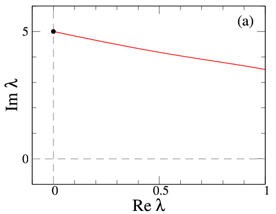
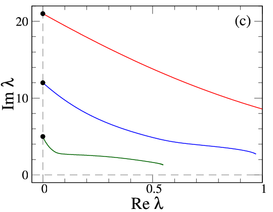
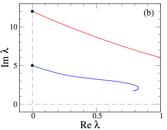
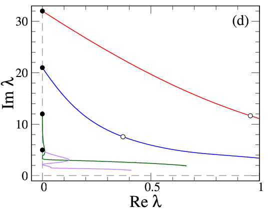
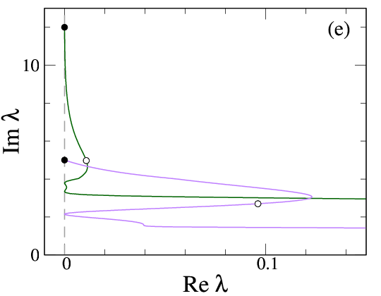
Figure 3. Eigenvalues of the linearized operator J​ℒJ\mathcal{L} around the bifurcated solitary wave born at β1=β1(ℓ)\beta_{1}=\beta_{1}^{(\ell)} for (ω,s,β2)=(1,4,2)(\omega,s,\beta_{2})=(1,4,2): (a) ℓ=1\ell=1; (b) ℓ=2\ell=2; (c) ℓ=3\ell=3; (d) and (e) ℓ=4\ell=4. Plate (e) is an enlargement of plate (d). The red, blue, green, and purple lines represent the eigenvalues of J​ℒJ\mathcal{L} with k=0,1,2k=0,1,2, and 33, respectively. The bullet ‘∙\bullet’ represents the loci of the eigenvalues at β1=β1(ℓ)\beta_{1}=\beta_{1}^{(\ell)}. In plates (d) and (e), the circle ‘∘\circ’ represents the loci of the eigenvalues at the saddle-node bifurcation point β1≈19.41626\beta_{1}\approx 19.41626. Each curve was computed from β1=β1(ℓ)\beta_{1}=\beta_{1}^{(\ell)} to 100100.
Refer to caption
Refer to caption
Refer to caption
Refer to caption
Refer to caption
Figure 4. Profiles of the eigenfunctions of the eigenvalue problem (2.7) for ℓ=2\ell=2 at β1=12\beta_{1}=12 with (ω,s,β2)=(1,4,2)(\omega,s,\beta_{2})=(1,4,2): (a) |ψ1||\psi_{1}|; (b) |ψ2||\psi_{2}|; (c) |ψ3||\psi_{3}|; (d) |ψ4||\psi_{4}|; (e) Ψ\Psi. The red and blue lines, respectively, represent the eigenfunctions for the curves emerging from 12​i12\mathrm{i} and 5​i5\mathrm{i} in Fig. 3(b).

Figure 3 shows how the eigenvalues of J​ℒJ\mathcal{L} for the bifurcated solitary wave on each branch change, where x±=±11x_{\pm}=\pm 11 was taken. We only display the eigenvalues with Re​λ,Im​λ≥0\mathrm{Re}\,\lambda,\mathrm{Im}\,\lambda\geq 0 since the spectra of J​ℒJ\mathcal{L} are symmetric, as stated in Section 2. For the bifurcated solitary wave born at β1=β1(ℓ)\beta_{1}=\beta_{1}^{(\ell)}, all eigenvalues of J​ℒJ\mathcal{L} at β1=β1(ℓ)\beta_{1}=\beta_{1}^{(\ell)} are given by

λ=\displaystyle\lambda= ±i⁡(s−ω​(s/ω+ℓ−k)2),\displaystyle\pm\mathrm{i}(s-\omega(\sqrt{s/\omega}+\ell-k)^{2}),
k∈{0,1,…,⌊s/ω⌋+ℓ}∖{s/ω+ℓ},\displaystyle k\in\{0,1,\ldots,\lfloor\sqrt{s/\omega}\rfloor+\ell\}\setminus\{\sqrt{s/\omega}+\ell\}, (3.12)

(see (2.11)) and they immediately disappear for k≥ℓk\geq\ell when β1\beta_{1} changes from β1(ℓ)\beta_{1}^{(\ell)} (see Remark 7.9 of [13]). The loci of the eigenvalues of J​ℒJ\mathcal{L} leaving the imaginary axis from (3.12) when β1\beta_{1} changes from β1(ℓ)\beta_{1}^{(\ell)} are plotted for k=0k=0 and ℓ=1\ell=1 in Fig. 3(a); for k=0,1k=0,1 and ℓ=2\ell=2 in Fig. 3(b); for k=0,1,2k=0,1,2 and ℓ=3\ell=3 in Fig. 3(c); and k=0,1,2,3k=0,1,2,3 and ℓ=4\ell=4 in Figs. 3(d) and (e). Each curve was computed from β1=β1(ℓ)\beta_{1}=\beta_{1}^{(\ell)} to 100100. Although (3.1) and (3.6) are highly degenerate at the bifurcation point β1=β1(ℓ)\beta_{1}=\beta_{1}^{(\ell)} since two branches of eigenfunctions are also created there, continuation of their solutions by AUTO succeeded from there. These results indicate that the real parts of the eigenvalues become positive and the bifurcated solitary waves are unstable when β1≠β1(ℓ)\beta_{1}\neq\beta_{1}^{(\ell)}, as stated in Theorem 2.2.

On the other hand, the computed eigenvalues at β1=50\beta_{1}=50 were almost the same as at β1=100\beta_{1}=100 for all computed branches. So the eigenvalues are thought to converge to certain values as β1→∞\beta_{1}\to\infty. See, e.g., the blue line (k=1k=1) in Fig. 3(b), the blue and green lines (k=1k=1 and 22) in Fig. 3(c), and the green and purple lines (k=2k=2 and 33) in Fig. 3(d). The reason is that as stated above, as β1→∞\beta_{1}\to\infty, the bifurcated homoclinic solutions converge to a certain profile, say (U∞​(x),V∞​(x))(U_{\infty}(x),V_{\infty}(x)), with a scaling of 1/β11/\sqrt{\beta_{1}} and the operators ℒ±\mathcal{L}_{\pm} in J​ℒJ\mathcal{L} with (2.5) converge to

ℒ+=(−∂x2+ω−V∞2−2​U∞​V∞−2​U∞​V∞−∂x2+s−U∞2),\displaystyle\mathcal{L}_{+}=\begin{pmatrix}-\partial_{x}^{2}+\omega-V_{\infty}^{2}&-2U_{\infty}V_{\infty}\\ -2U_{\infty}V_{\infty}&-\partial_{x}^{2}+s-U_{\infty}^{2}\end{pmatrix},
ℒ−=(−∂x2+ω−V∞200−∂x2+s−U∞2).\displaystyle\mathcal{L}_{-}=\begin{pmatrix}-\partial_{x}^{2}+\omega-V_{\infty}^{2}&0\\ 0&-\partial_{x}^{2}+s-U_{\infty}^{2}\end{pmatrix}.

Note that (U,V)→0(U,V)\to 0 while β1​(U,V)→(U∞,V∞)\sqrt{\beta_{1}}(U,V)\to(U_{\infty},V_{\infty}).

In Figs. 3(d) and (e) four eigenvalues for the bifurcated solitary wave on the fifth branch (ℓ=4\ell=4) are displayed and their values at β1=β1SN≈19.41626\beta_{1}=\beta_{1}^{\mathrm{SN}}\approx 19.41626, at which a saddle-node bifurcation occurs (see Fig. 1(a)), are plotted as a circle ‘∘\circ’. In particular, the solitary wave seems not to change its stability type at the saddle-node bifurcation point since all the eigenvalues are far from the imaginary axis. On the other hand, according to Theorem 2.4 of [2], the VE (2.1) around the corresponding homoclinic solution has two linearly independent solutions there since no bifurcation occurs if it does not, so that the geometrical multiplicity of the zero eigenvalue of J​ℒJ\mathcal{L} increases by one. So we suspect that for the zero eigenvalue a generalized eigenfuntion turns to an eigenfunction there, as suggested from Yang’s result [17] for general single NLS equations with external potentials. This suspicion will be numerically proven true in the next section.

Figure 4 displays the absolute value of each component of the corresponding eigenfunction ψ=(ψ1,…,ψ4)T\psi=(\psi_{1},\ldots,\psi_{4})^{\mathrm{T}} for ℓ=2\ell=2 at β1=14\beta_{1}=14. In Fig. 4(e), the profiles of Ψ⁡(x)\Psi(x) for ℓ=2\ell=2, which are given by (2.12) and (2.13) with k=0k=0 and 11, and represent the eigenfunctions associated with the eigenvalues λ=12​i\lambda=12\mathrm{i} and 5​i5\mathrm{i} there as ψ=(0,Ψ,0,i​Ψ)T\psi=(0,\Psi,0,\mathrm{i}\Psi)^{\mathrm{T}}, are plotted as the red and blue lines, respectively. We see that the eigenfunctions considerably changes from those at the bifurcation point β1=β1(2)\beta_{1}=\beta_{1}^{(2)}.

4. Computations of generalized eigenfunctions for the zero eigenvalues

In this section, for the eigenvalue problem (2.7), we give some numerical computation results for its generalized eigenfunction associated with the zero eigenvalue which turns to an eigenfunction at the saddle-node bifurcation point. These results will demonstrate the correctness of our suspicion stated above on the saddle-node bifurcation observed in Fig. 1(a): the geometric multiplicity of the zero eigenvalue increases by one but the number of eigenvalues counted with their multiplicity on the imaginary axis does not change, so that the solitary wave does not change its stability type at the bifurcation point.

4.1. Numerical Approach

We first recall that φj\varphi_{j} and χj\chi_{j}, j=1,2,3j=1,2,3, can be the eigenfunctions and generalized eigenfunctions of (2.7) associated with the zero eigenvalue which are given by (2.9) and (2.10), respectively, such that J​ℒ​χj=φjJ\mathcal{L}\chi_{j}=\varphi_{j}. Moreover, the first and second components of χ1\chi_{1} are zero while the third and fourth components of χ2\chi_{2} and χ3\chi_{3} are zero. Hence, if a generalized eigenfunction χ\chi for the zero eigenvalue becomes an eigenfunction at the saddle-node bifurcation point β1SN\beta_{1}^{\mathrm{SN}}, then χ\chi can be written as a linear combination of χ2\chi_{2} and χ3\chi_{3}. This means that the geometric multiplicity is four at β1=β1SN\beta_{1}=\beta_{1}^{\mathrm{SN}} but three at β1≠β1SN\beta_{1}\neq\beta_{1}^{\mathrm{SN}} while the algebraic multiplicity is six for both cases. So we want to compute a generalized eigenfunction satisfying

J​ℒ​ψ=ε1​((1−ε2)​φ2+ε2​φ3)\displaystyle J\mathcal{L}\psi=\varepsilon_{1}((1-\varepsilon_{2})\varphi_{2}+\varepsilon_{2}\varphi_{3}) (4.1)

where ε1,ε2∈ℝ\varepsilon_{1},\varepsilon_{2}\in\mathbb{R} are constants. If ε1=0\varepsilon_{1}=0, then ψ\psi becomes an eigenfunction. If ε2=0\varepsilon_{2}=0 and 11 with ε1=1\varepsilon_{1}=1, then ψ=χ2\psi=\chi_{2} and χ3\chi_{3}, respectively, satisfy (4.1).

Combining (3.1) and (4.1), we write our problem as

(z′η′)=g⁡(z,η,β1,ε1,ε2),z=(z1,z2,z3,z4)T,η=(η1,η2,η3,η4)T∈ℝ4,\displaystyle\begin{pmatrix}z^{\prime}\\ \eta^{\prime}\end{pmatrix}=g(z,\eta;\beta_{1},\varepsilon_{1},\varepsilon_{2}),\quad z=(z_{1},z_{2},z_{3},z_{4})^{\mathrm{T}},\eta=(\eta_{1},\eta_{2},\eta_{3},\eta_{4})^{\mathrm{T}}\in\mathbb{R}^{4}, (4.2)

and numerically compute a homoclinic solution to (4.2) satisfying

limx→±∞z⁡(x)=limx→±∞η⁡(x)=0,\displaystyle\lim_{x\to\pm\infty}z(x)=\lim_{x\to\pm\infty}\eta(x)=0, (4.3)

where ηj=ψj\eta_{j}=\psi_{j}, j=1,2j=1,2, and

g⁡(z,η,β1,ε1,ε2)\displaystyle g(z,\eta;\beta_{1},\varepsilon_{1},\varepsilon_{2})
⋅⋅=(z3z4ω​z1−(z12+β1​z22)​z1+d1​z3s​z2−(β1​z12+β2​z22)​z2+d1​z4η3η4ω​η1−(3​z12+β1​z22)​η1−2​β1​z1​z2​η2+ε1​(1−ε2)​z1+d2​z3s​η2−2​β1​z1​z2​η1−(β1​z12+3​β2​z22)​η2+ε1​ε2​z2+d2​z4)\displaystyle\mathrel{\hbox to0.0pt{\raisebox{1.29167pt}{$\cdot$}\hss}\raisebox{-1.29167pt}{$\cdot$}}=\begin{pmatrix}z_{3}\\ z_{4}\\ \omega z_{1}-(z_{1}^{2}+\beta_{1}z_{2}^{2})z_{1}+d_{1}z_{3}\\ sz_{2}-(\beta_{1}z_{1}^{2}+\beta_{2}z_{2}^{2})z_{2}+d_{1}z_{4}\\ \eta_{3}\\ \eta_{4}\\ \omega\eta_{1}-(3z_{1}^{2}+\beta_{1}z_{2}^{2})\eta_{1}-2\beta_{1}z_{1}z_{2}\eta_{2}+\varepsilon_{1}(1-\varepsilon_{2})z_{1}+d_{2}z_{3}\\ s\eta_{2}-2\beta_{1}z_{1}z_{2}\eta_{1}-(\beta_{1}z_{1}^{2}+3\beta_{2}z_{2}^{2})\eta_{2}+\varepsilon_{1}\varepsilon_{2}z_{2}+d_{2}z_{4}\end{pmatrix}

with dummy parameters d1,d2d_{1},d_{2}. Here the first and second components of (4.1) and the third and fourth components of ψ\psi have been eliminated since the first and second components of both φ2\varphi_{2} and φ3\varphi_{3} and the third and fourth components of both χ2\chi_{2} and χ3\chi_{3} are zero. The fact that the third and fourth components of φ2\varphi_{2} are (U⁡(x),0)(U(x),0) and those of φ3\varphi_{3} are (0,V⁡(x))(0,V(x)) has also been used (see (2.10)). We easily see that a homoclinic solution persists in (4.2) when one of the other parameters changes only if d1=d2=0d_{1}=d_{2}=0, as in (3.1).

Let E^s\hat{E}^{\mathrm{s}} and E^u\hat{E}^{\mathrm{u}} be, respectively, the four-dimensional stable and unstable subspaces of the linearized system at the origin for (4.2),

(δ​z′δ​η′)=Dz,η​g​(0,0,β1,ε1,ε2)​(δ​zδ​η)\displaystyle\begin{pmatrix}\delta z^{\prime}\\ \delta\eta^{\prime}\end{pmatrix}=\mathrm{D}_{z,\eta}g(0,0;\beta_{1},\varepsilon_{1},\varepsilon_{2})\begin{pmatrix}\delta z\\ \delta\eta\end{pmatrix}

with

Dz,η​g​(0,0,β1,ε1,ε2)=(00100001ω0d100s0d1O400000000ε1​(1−ε2)0d200ε1​ε20d200100001ω0000s00).\displaystyle\mathrm{D}_{z,\eta}g(0,0;\beta_{1},\varepsilon_{1},\varepsilon_{2})=\left(\begin{array}[]{c|c}\begin{array}[]{cccc}0&0&1&0\\ 0&0&0&1\\ \omega&0&d_{1}&0\\ 0&s&0&d_{1}\end{array}&O_{4}\\ \hline\cr\begin{array}[]{cccc}0&0&0&0\\ 0&0&0&0\\ \varepsilon_{1}(1-\varepsilon_{2})&0&d_{2}&0\\ 0&\varepsilon_{1}\varepsilon_{2}&0&d_{2}\end{array}&\begin{array}[]{cccc}0&0&1&0\\ 0&0&0&1\\ \omega&0&0&0\\ 0&s&0&0\end{array}\end{array}\right).

As in Section 3, we approximate the homoclinic solution (z⁡(x),η⁡(x))T(z(x),\eta(x))^{\mathrm{T}} to (4.2) satisfying (4.3), so that it starts on E^u\hat{E}^{\mathrm{u}} near the origin at x−x_{-} and arrives on E^s\hat{E}^{\mathrm{s}} near the origin at x+x_{+}. So we look for a solution to (4.2) satisfying

L^s​(z⁡(x−)η⁡(x−))=0,L^u​(z⁡(x+)η⁡(x+))=0,\displaystyle\hat{L}^{\mathrm{s}}\begin{pmatrix}z(x_{-})\\ \eta(x_{-})\end{pmatrix}=0,\quad\hat{L}^{\mathrm{u}}\begin{pmatrix}z(x_{+})\\ \eta(x_{+})\end{pmatrix}=0, (4.4)

where

L^s⋅⋅=(−d1/2−ω+(d1/2)200−d1/2−s+(d1/2)2L^31s00L^42sL^−),\displaystyle\hat{L}^{\mathrm{s}}\mathrel{\hbox to0.0pt{\raisebox{1.29167pt}{$\cdot$}\hss}\raisebox{-1.29167pt}{$\cdot$}}=\left(\begin{array}[]{c|c}\begin{array}[]{cc}-d_{1}/2-\sqrt{\omega+(d_{1}/2)^{2}}&0\\ 0&-d_{1}/2-\sqrt{s+(d_{1}/2)^{2}}\\ \hat{L}^{\mathrm{s}}_{31}&0\\ 0&\hat{L}^{\mathrm{s}}_{42}\end{array}&\hat{L}_{-}\end{array}\right),
L^u⋅⋅=(−d1/2+ω+(d1/2)200−d1/2+s+(d1/2)2L^31u00L^42uL^+)\displaystyle\hat{L}^{\mathrm{u}}\mathrel{\hbox to0.0pt{\raisebox{1.29167pt}{$\cdot$}\hss}\raisebox{-1.29167pt}{$\cdot$}}=\left(\begin{array}[]{c|c}\begin{array}[]{cc}-d_{1}/2+\sqrt{\omega+(d_{1}/2)^{2}}&0\\ 0&-d_{1}/2+\sqrt{s+(d_{1}/2)^{2}}\\ \hat{L}^{\mathrm{u}}_{31}&0\\ 0&\hat{L}^{\mathrm{u}}_{42}\end{array}&\hat{L}_{+}\end{array}\right)

with

L^31s=−ε1​(1−ε2)−d2​ω2​ω+−ε1​(1−ε2)+d2​ωω​ω+(d1/2)2−ωd1,L^42s=−ε1​ε2−d2​s2​s+−ε1​ε2+d2​ss​s+(d1/2)2−sd1,L^31u=ε1​(1−ε2)−d2​ω2​ω+ε1​(1−ε2)+d2​ωω​ω+(d1/2)2−ωd1,L^42u=ε1​ε2−d2​s2​s+ε1​ε2+d2​ss​s+(d1/2)2−sd1\begin{split}&\hat{L}^{\mathrm{s}}_{31}=\frac{-\varepsilon_{1}(1-\varepsilon_{2})-d_{2}\sqrt{\omega}}{2\sqrt{\omega}}+\frac{-\varepsilon_{1}(1-\varepsilon_{2})+d_{2}\sqrt{\omega}}{\sqrt{\omega}}\frac{\sqrt{\omega+(d_{1}/2)^{2}}-\sqrt{\omega}}{d_{1}},\\ &\hat{L}^{\mathrm{s}}_{42}=\frac{-\varepsilon_{1}\varepsilon_{2}-d_{2}\sqrt{s}}{2\sqrt{s}}+\frac{-\varepsilon_{1}\varepsilon_{2}+d_{2}\sqrt{s}}{\sqrt{s}}\frac{\sqrt{s+(d_{1}/2)^{2}}-\sqrt{s}}{d_{1}},\\ &\hat{L}^{\mathrm{u}}_{31}=\frac{\varepsilon_{1}(1-\varepsilon_{2})-d_{2}\sqrt{\omega}}{2\sqrt{\omega}}+\frac{\varepsilon_{1}(1-\varepsilon_{2})+d_{2}\sqrt{\omega}}{\sqrt{\omega}}\frac{\sqrt{\omega+(d_{1}/2)^{2}}-\sqrt{\omega}}{d_{1}},\\ &\hat{L}^{\mathrm{u}}_{42}=\frac{\varepsilon_{1}\varepsilon_{2}-d_{2}\sqrt{s}}{2\sqrt{s}}+\frac{\varepsilon_{1}\varepsilon_{2}+d_{2}\sqrt{s}}{\sqrt{s}}\frac{\sqrt{s+(d_{1}/2)^{2}}-\sqrt{s}}{d_{1}}\end{split} (4.5)

and

L^±=(10000001000000±ω010000±s01).\hat{L}_{\pm}=\begin{pmatrix}1&0&0&0&0&0\\ 0&1&0&0&0&0\\ 0&0&\pm\sqrt{\omega}&0&1&0\\ 0&0&0&\pm\sqrt{s}&0&1\end{pmatrix}.

Here L^+\hat{L}_{+} and L^−\hat{L}_{-} are 4×84\times 8 real matrices consisting of bases in the subspaces spanned by row eigenvectors for Dz,η​g​(0,0,β1,ε1,ε2)\mathrm{D}_{z,\eta}g(0,0;\beta_{1},\varepsilon_{1},\varepsilon_{2}) such that the associated eigenvalues have negative and positive real parts, respectively. In the computation, the distances |z⁡(x±)||z(x_{\pm})| should be kept small but |η⁡(x±)||\eta(x_{\pm})| do not have to be small necessarily like |ζR​(x±)|,|ζI​(x±)||\zeta_{\mathrm{R}}(x_{\pm})|,|\zeta_{\mathrm{I}}(x_{\pm})| in Section 3.

Furthermore, to monitor the L2L^{2} norm of (η1,η2)T(\eta_{1},\eta_{2})^{\mathrm{T}}, we add a parameter c1∈ℝc_{1}\in\mathbb{R} and the integral condition

∫x−x+(η1​(x)2+η2​(x)2)​𝑑x=c1.\displaystyle\int_{x_{-}}^{x_{+}}\bigl(\eta_{1}(x)^{2}+\eta_{2}(x)^{2}\bigr)\mathrm{d}x=c_{1}. (4.6)

From (2.9) we see that if (z⁡(x),η⁡(x))(z(x),\eta(x)) is a solution to (4.2) with d2=0d_{2}=0, then so is (z⁡(x),η⁡(x)+α​η0​(t))(z(x),\eta(x)+\alpha\eta_{0}(t)) for any α∈ℝ\alpha\in\mathbb{R}, where η0​(x)=(U′​(x),V′​(x),U′′​(x),V′′​(x))\eta_{0}(x)=(U^{\prime}(x),V^{\prime}(x),U^{\prime\prime}(x),V^{\prime\prime}(x)). To monitor the dependence of η⁡(x)\eta(x) on η0​(x)\eta_{0}(x), we add a parameter c2∈ℝc_{2}\in\mathbb{R} and the integral condition

∫x−x+(η1​(x)​z3​(x)+η2​(x)​z4​(x))​𝑑x=c2.\displaystyle\int_{x_{-}}^{x_{+}}\bigl(\eta_{1}(x)z_{3}(x)+\eta_{2}(x)z_{4}(x)\bigr)\mathrm{d}x=c_{2}. (4.7)

If c2=0c_{2}=0, then η⁡(x)\eta(x) is orthogonal to η0​(x)\eta_{0}(x). To eliminate the multiplicity of solutions due to the translational symmetry of (1.4), we also add the integral condition (3.5), as in Section 3.1.

4.2. Numerical Results

Refer to caption
Figure 5. Partial enlargement of Fig. 1(a): Bifurcation diagram of solitary waves in (1). The labeled solutions in Table 2 are located.
Refer to caption
Refer to caption
Refer to caption
Figure 6. Numerically computed homoclinic solutions to (1.4) for (ω,s,β2)=(1,4,2)(\omega,s,\beta_{2})=(1,4,2): (a) β1=20\beta_{1}=20; (b) β1=β1SN\beta_{1}=\beta_{1}^{\mathrm{SN}}; (c) β1=20\beta_{1}=20. The red and blue lines, respectively, represents the UU- and VV-components. The solutions in plates (a) and (c) are, respectively, denoted by ∙\bullet and ■\blacksquare on the branch in Fig. 5.

We set ω=1\omega=1, s=4s=4, and β2=2\beta_{2}=2 as in Section 3.2. Figure 5 is a partial enlargement of Fig. 1(a) in which the pitchfork and saddle-node bifurcation points on the fifth branch are contained. The corresponding homoclinic solutions to (1.4) on the branch are displayed in Fig. 6. We carried out numerical computations stated in Section 4.1 along the branch beyond the saddle-node bifurcation point β1=β1SN≈19.41626\beta_{1}=\beta_{1}^{\mathrm{SN}}\approx 19.41626. We also used the computer tool AUTO [4] to obtain numerical solutions to (4.2) satisfying the boundary condition (4.4) under the integral conditions (3.5), (4.6), and (4.7), as in Section 3.

Table 2. Summary of the numerical continuations. Here c0≈0.074836c_{0}\approx 0.074836 (see (4.9)).
Run Varied parameter Fixed parameter values Starting Terminating
no. β1\beta_{1} ε2\varepsilon_{2} c1c_{1} c2c_{2} solution solution
1 c1=c0→1c_{1}=c_{0}\to 1 2020 00 - c0c_{0} A B
2 c2=c0→0c_{2}=c_{0}\to 0 2020 00 11 - B C1\mathrm{C}_{1}
3 β1=20→β1SN→20\beta_{1}=20\to\beta_{1}^{\mathrm{SN}}\to 20 - 00 11 00 C1\mathrm{C}_{1} D1\mathrm{D}_{1}
4 ε2=0→1\varepsilon_{2}=0\to 1 2020 - 11 00 C1\mathrm{C}_{1} C2\mathrm{C}_{2}
5 β1=20→β1SN→20\beta_{1}=20\to\beta_{1}^{\mathrm{SN}}\to 20 - 11 11 00 C2\mathrm{C}_{2} D2\mathrm{D}_{2}

Since at the fifth pitchfork bifurcation point β1=β1(4)=21\beta_{1}=\beta_{1}^{(4)}=21, dimKer⁡J​ℒ\dim\Ker J\mathcal{L} increases by two and consequently (4.2) is highly degenerate, it is difficult to continue a branch of solutions in the boundary value problem beyond there. From this reason we computed the solution branch after the pitchfork bifurcation occurs. As the starting solution in a series of numerical continuations, we adopted

z=(U⁡(x),V⁡(x),U′​(x),V′​(x))Tη=(U′​(x),V′​(x),U′′​(x),V′′​(x))T\displaystyle z=(U(x),V(x),U^{\prime}(x),V^{\prime}(x))^{\mathrm{T}}\quad\eta=(U^{\prime}(x),V^{\prime}(x),U^{\prime\prime}(x),V^{\prime\prime}(x))^{\mathrm{T}} (4.8)

at β1=20\beta_{1}=20 on the branch with ε1,ε2,d1,d2=0\varepsilon_{1},\varepsilon_{2},d_{1},d_{2}=0, where U⁡(x),V⁡(x),U′​(x)U(x),V(x),U^{\prime}(x), and V′​(x)V^{\prime}(x) were numerically obtained along with

U′′​(x)=ω​U​(x)−(U​(x)2+β1​V​(x)2)​U​(x),\displaystyle U^{\prime\prime}(x)=\omega U(x)-(U(x)^{2}+\beta_{1}V(x)^{2})U(x),
V′′​(x)=s​V​(x)−(β1​U​(x)2+β2​V​(x)2)​V​(x)\displaystyle V^{\prime\prime}(x)=sV(x)-(\beta_{1}U(x)^{2}+\beta_{2}V(x)^{2})V(x)

in advance by another numerical continuation for the boundary value problem of (3.1) with (3.4). We chose x±=±9x_{\pm}=\pm 9 and executed five runs in total. All of the runs are summarized in Table 2. In the numerical continuations, β1\beta_{1}, ε2\varepsilon_{2}, c1c_{1} or c2c_{2} was varied while ε1\varepsilon_{1}, d1d_{1}, and d2d_{2} were taken as the free parameters. The distances |z⁡(x±)||z(x_{\pm})| were monitored along with |η⁡(x±)||\eta(x_{\pm})| and kept small (≈10−3\approx 10^{-3}) during the computations. Moreover, since d1d_{1} is very small (it should be zero theoretically), the approximations

ω+(d1/2)2−ωd1≈d18​ω,s+(d1/2)2−sd1≈d18​s,\frac{\sqrt{\omega+(d_{1}/2)^{2}}-\sqrt{\omega}}{d_{1}}\approx\frac{d_{1}}{8\sqrt{\omega}},\quad\frac{\sqrt{s+(d_{1}/2)^{2}}-\sqrt{s}}{d_{1}}\approx\frac{d_{1}}{8\sqrt{s}},

were used in the computations of (4.5).

In the first run, we took the numerical solution (4.8) with (β1,ε2)=(20,0)(\beta_{1},\varepsilon_{2})=(20,0) and

c1=c2=∫x−x+(U′​(x)2+V′​(x)2)​𝑑x=:c0≈0.074836\displaystyle c_{1}=c_{2}=\int_{x_{-}}^{x_{+}}\bigl(U^{\prime}(x)^{2}+V^{\prime}(x)^{2}\bigr)\,\mathrm{d}x=:c_{0}\approx 0.074836 (4.9)

labeled by ‘A’ as the starting solution and continued it from c1=c0c_{1}=c_{0} to 11 for β1,ε2,c2\beta_{1},\varepsilon_{2},c_{2} fixed. The solution calculated at c1=1c_{1}=1, the (η1,η2)(\eta_{1},\eta_{2})-components of which are normalized, is labeled by ‘B’. In the second run, we fixed (β1,ε2,c1)=(20,0,1)(\beta_{1},\varepsilon_{2},c_{1})=(20,0,1) and followed the solution ‘B’ from c2=c0c_{2}=c_{0} to 00. The solution calculated at c2=0c_{2}=0, for which (η1​(x),η2​(x))(\eta_{1}(x),\eta_{2}(x)) is orthogonal to (z3,z4)=(U′​(x),V′​(x))(z_{3},z_{4})=(U^{\prime}(x),V^{\prime}(x)) by (4.7), is labeled by ‘C1\mathrm{C}_{1}’. In the third run, we fixed (ε2,c1,c2)=(0,1,0)(\varepsilon_{2},c_{1},c_{2})=(0,1,0) and followed the solution ‘C1\mathrm{C}_{1}’ for J​ℒ​ψ=ε1​φ2J\mathcal{L}\psi=\varepsilon_{1}\varphi_{2} (see (4.1)) from β1=20\beta_{1}=20 to β1SN\beta_{1}^{\mathrm{SN}} and from β1SN\beta_{1}^{\mathrm{SN}} to 2020. The finally obtained solution is labeled by ‘D1\mathrm{D}_{1}’. See Fig. 5.

Refer to captionRefer to caption
Figure 7. Numerically computed generalized eigenfunctions satisfying (4.1) with ε2=0\varepsilon_{2}=0 for (ω,s,β2)=(1,4,2)(\omega,s,\beta_{2})=(1,4,2): (a) Solution branch C1​D1\mathrm{C}_{1}\mathrm{D}_{1}; (b) β1=20\beta_{1}=20 (at C1\mathrm{C}_{1}); (c) β1=β1SN\beta_{1}=\beta_{1}^{\mathrm{SN}}; (d) β1=20\beta_{1}=20 (at D1\mathrm{D}_{1}). The red and blue lines, respectively, represent the first and second components.

Figure 7 shows generalized eigenfunctions satisfying (4.1) with ε2=0\varepsilon_{2}=0 along with the solution branch obtained from the third run. In particular, at the saddle-node bifurcation point β1=β1SN\beta_{1}=\beta_{1}^{\mathrm{SN}}, we observe ε1=0\varepsilon_{1}=0, so that the generalized eigenfunction expressed as a linear combination of φ1\varphi_{1} and χ2\chi_{2} becomes an eigenfunction for the zero eigenvalue in the eigenvalue problem (2.7), as we suspect. Thus, the corresponding solitary wave does not change its stability type at β1=β1SN\beta_{1}=\beta_{1}^{\mathrm{SN}}: the number of eigenvalues with positive real parts does not change. This is similar to Yang’s result [17] for general single NLS equations with external potentials.

In the fourth run, we fixed (β1,c1,c2)=(20,1,0)(\beta_{1},c_{1},c_{2})=(20,1,0) and followed the solution ‘C1\mathrm{C}_{1}’ from ε2=0\varepsilon_{2}=0 to 11 for β1=20\beta_{1}=20 fixed. The solution calculated at ε2=1\varepsilon_{2}=1 is labeled by ‘C2\mathrm{C}_{2}’. In the last run, we fixed (ε2,c1,c2)=(1,1,0)(\varepsilon_{2},c_{1},c_{2})=(1,1,0) and followed the solution ‘C2\mathrm{C}_{2}’ for J​ℒ​ψ=ε1​φ3J\mathcal{L}\psi=\varepsilon_{1}\varphi_{3} (see (4.1)) from β1=20\beta_{1}=20 to β1SN\beta_{1}^{\mathrm{SN}} and from β1SN\beta_{1}^{\mathrm{SN}} to 2020. The finally obtained solution is labeled by ‘D2\mathrm{D}_{2}’. See Fig. 5.

Refer to captionRefer to caption
Figure 8. Numerically computed generalized eigenfunctions satisfying (4.1) with ε2=1\varepsilon_{2}=1 for (ω,s,β2)=(1,4,2)(\omega,s,\beta_{2})=(1,4,2): (a) Solution branch C2​D2\mathrm{C}_{2}\mathrm{D}_{2}; (b) β1=20\beta_{1}=20 (at C2\mathrm{C}_{2}); (c) β1=β1SN\beta_{1}=\beta_{1}^{\mathrm{SN}}; (d) β1=20\beta_{1}=20 (at D2\mathrm{D}_{2}). The red and blue lines, respectively, represent the first and second components.

Figure 8 shows generalized eigenfunctions satisfying (4.1) with ε2=1\varepsilon_{2}=1 along with the solution branch obtained from the last run. In particular, at the saddle-node bifurcation point β1=β1SN\beta_{1}=\beta_{1}^{\mathrm{SN}}, we observe ε1=0\varepsilon_{1}=0, so that the generalized eigenfunction expressed as a linear combination of φ1\varphi_{1} and χ3\chi_{3} becomes an eigenfunction for the zero eigenvalue in the eigenvalue problem (2.7), again. Moreover, the eigenfunction of Fig. 8(c) coincide with that of Fig. 7(c) up to multiplication by −1-1. Thus, the generalized eigenfunctions for φ2\varphi_{2} and φ3\varphi_{3} give the same eigenfunction at β1=β1SN\beta_{1}=\beta_{1}^{\mathrm{SN}}, and dimKer⁡J​ℒ\dim\Ker J\mathcal{L} increases by one at β1=β1SN\beta_{1}=\beta_{1}^{\mathrm{SN}}.

We close this paper with showing that dimgKer⁡J​ℒ\dim\gKer J\mathcal{L} does not change at β1SN\beta_{1}^{\mathrm{SN}} although the two linearly independent generalized eigenfunctions were observed to converge to the eigenfunction as β1→β1SN\beta_{1}\to\beta_{1}^{\mathrm{SN}}.

Fix β1=β1SN\beta_{1}=\beta_{1}^{\mathrm{SN}}. Let (η1SN,η2SN)(\eta_{1}^{\mathrm{SN}},\eta_{2}^{\mathrm{SN}}) denote the (η1,η2)(\eta_{1},\eta_{2})-components of the solution to (4.2) with (ε1,c2)=(0,0)(\varepsilon_{1},c_{2})=(0,0) corresponding to an eigenfunction of (2.7) for the zero eigenvalue, such as plotted in Figs. 7(c) and 8(c). We see that (η1SN,η2SN)∈Ker⁡ℒ+(\eta_{1}^{\mathrm{SN}},\eta_{2}^{\mathrm{SN}})\in\Ker\mathcal{L}_{+}, where ℒ+\mathcal{L}_{+} is the linear operator given in (2.6). Moreover, Ker⁡ℒ+\Ker\mathcal{L}_{+} is of dimension two at most since the corresponding four-dimensional system of first-order ODEs converges to (3.3) as x→±∞x\to\pm\infty and the stable and unstable subspaces of the origin in (3.3) are of dimension two (dimEs=dimEu=2\dim E^{\mathrm{s}}=\dim E^{\mathrm{u}}=2). So {(U′,V′),(η1SN,η2SN)}\{(U^{\prime},V^{\prime}),(\eta_{1}^{\mathrm{SN}},\eta_{2}^{\mathrm{SN}})\} is a basis of Ker⁡ℒ+\Ker\mathcal{L}_{+}. Similarly, Ker⁡ℒ−\Ker\mathcal{L}_{-} is of dimension two at most and {(U,0),(0,V)}\{(U,0),(0,V)\} is its basis, where ℒ−\mathcal{L}_{-} is the linear operator given in (2.6). Thus, Ker⁡J​ℒ=Ker⁡ℒ+⊕Ker⁡ℒ−\Ker J\mathcal{L}=\Ker\mathcal{L}_{+}\oplus\Ker\mathcal{L}_{-} is of dimension four and spanned by

{φ1,(η1SN,η2SN,0,0)T,φ2,φ3},\displaystyle\{\varphi_{1},(\eta_{1}^{\mathrm{SN}},\eta_{2}^{\mathrm{SN}},0,0)^{\mathrm{T}},\varphi_{2},\varphi_{3}\},

where φj\varphi_{j}, j=1,2,3j=1,2,3, were given in (2.9).

To determine gKer⁡J​ℒ\gKer J\mathcal{L}, we consider the solvability of

ℒ−​(ζ1ζ2)=α1​(U′V′)+α2​(η1SNη2SN)\displaystyle\mathcal{L}_{-}\begin{pmatrix}\zeta_{1}\\ \zeta_{2}\end{pmatrix}=\alpha_{1}\begin{pmatrix}U^{\prime}\\ V^{\prime}\end{pmatrix}+\alpha_{2}\begin{pmatrix}\eta_{1}^{\mathrm{SN}}\\ \eta_{2}^{\mathrm{SN}}\end{pmatrix} (4.10)

and

ℒ+​(ζ1ζ2)=α1​(U0)+α2​(0V),\displaystyle\mathcal{L}_{+}\begin{pmatrix}\zeta_{1}\\ \zeta_{2}\end{pmatrix}=\alpha_{1}\begin{pmatrix}U\\ 0\end{pmatrix}+\alpha_{2}\begin{pmatrix}0\\ V\end{pmatrix}, (4.11)

where αj\alpha_{j}, j=1,2j=1,2, are constants. Note that nontrivial solutions to (4.10) and (4.11) provide elements of gKer⁡J​ℒ\gKer J\mathcal{L}. Numerical integrations carried out in the software AUTO yielded

I1=∫x−x+η1SN​(x)​U​(x)​𝑑x≈1.492,I2=∫x−x+η2SN​(x)​V​(x)​𝑑x≈−0.373,\displaystyle I_{1}=\int_{x_{-}}^{x_{+}}\eta_{1}^{\mathrm{SN}}(x)U(x)\,\mathrm{d}x\approx 1.492,\quad I_{2}=\int_{x_{-}}^{x_{+}}\eta_{2}^{\mathrm{SN}}(x)V(x)\,\mathrm{d}x\approx-0.373,

which indicates along with the Fredholm alternative theorem [7] that there exists an L2L^{2} solution to (4.10) (resp. to (4.11)) if and only if α2=0\alpha_{2}=0 (resp. I1​α1+I2​α2=0I_{1}\alpha_{1}+I_{2}\alpha_{2}=0). Actually, ζ=(−xU(x)/2,−xV(x)/2)\zeta=(-xU(x)/2,-xV(x)/2) is the solution to (4.10) with α2=0\alpha_{2}=0, and consequently it is reconfirmed that χ1∈gKer⁡J​ℒ\chi_{1}\in\gKer J\mathcal{L}. Thus, there exist two linearly independent generalized eigenfunctions and dimgKer⁡J​ℒ\dim\gKer J\mathcal{L} does not change at β1=β1SN\beta_{1}=\beta_{1}^{\mathrm{SN}}.

References

  • [1] J. Alexander, R. Gardner, and C. Jones, A topological invariant arising in the stability analysis of travelling waves, J. reine angew. Math., 410 (1990) 167–212.
  • [2] D. Blázquez-Sanz and K. Yagasaki, Analytic and algebraic conditions for bifurcations of homoclinic orbits I: Saddle equilibria, J. Differential Equations, 253 (2012) 2916–2950.
  • [3] A. Champneys, Y. Kuznetsov, and B. Sandstede, A numerical toolbox for homoclinic bifurcation analysis, Int. J. Bifurc. Chaos Appl. Sci. Eng., 6 (1996) 867–887.
  • [4] E. Doedel and B. Oldeman, AUTO-07P: Continuation and Bifurcation Software for Ordinary Differential Equations, 2012, available online from http://indy.cs.concordia.ca/auto.
  • [5] M. Grillakis, Analysis of the linearization around a critical point of an infinite dimensional Hamiltonian system, Commun. Pure Appl. Math., 43 (1990) 299–333.
  • [6] R. Jackson, On the mechanisms for instability of standing waves in nonlinearly coupled Schrödinger equations, Nonlinearity, 24 (2011) 2849–2873.
  • [7] T. Kapitula and K. Promislow, Spectral and Dynamical Stability of Nonlinear Waves, Springer, New York, 2013.
  • [8] Y. Li and K. Promislow, The mechanism of the polarizational mode instability in birefringent fiber optics, SIAM J. Math. Anal., 31 (2000) 1351–1373.
  • [9] D. Pelinovsky, Localization in Periodic Potentials: From Schrödinger Operators to the Gross-Pitaevskii Equation, Cambridge University Press, Cambridge, 2011.
  • [10] D. Pelinovsky and J. Yang, Internal oscillations and radiation damping of vector solitons, Stud. Appl. Math., 105 (2000) 245–276.
  • [11] D. Pelinovsky and J. Yang, Instabilities of multihump vector solitons in coupled nonlinear Schrödinger equations, Stud. Appl. Math., 115 (2005) 109–137.
  • [12] K. Yagasaki and S. Yamazoe, Numerical analyses for spectral stability of solitary waves near bifurcation points, Jpn J. Ind. Appl. Math., 38 (2021) 125–140.
  • [13] K. Yagasaki and S. Yamazoe, Bifurcations and spectral stability of solitary waves in coupled nonlinear Schrödinger equations, submitted for publication, arXiv:2005.10317v2.
  • [14] J. Yang, Classification of the solitary waves in coupled nonlinear Schrödinger equations, Physica D, 108 (1997) 92–112.
  • [15] J. Yang, Vector solitons and their internal oscilliations in birefringent nonlinear optical fibers, Stud. Appl. Math., 98 (1997) 61–97.
  • [16] J. Yang, Nonlinear Waves in Integrable and Nonintegrable Systems, SIAM, Philadelphia, PA, 2010.
  • [17] J. Yang, No stability switching at saddle-node bifurcations of solitary waves in generalized nonlinear Schrödinger equations, Phys. Rev. E, 85 (2012) 037602.