Spatial spread of COVID-19 outbreak in Italy using multiscale kinetic transport equations with uncertainty

We consider a population of commuters at position $x\in\Omega$ moving with velocity directions $v\in\mathbb{S}^{1}$ and denote the respective kinetic densities of susceptible (individuals who may be infected by the disease) by $f_{S}=f_{S}(x,v,t)$, exposed (individuals in the latent period, which are not yet infectious) by $f_{E}=f_{E}(x,v,t)$, severe symptomatic infected by $f_{I}=f_{I}(x,v,t)$, mildly symptomatic or asymptomatic infected by $f_{A}=f_{A}(x,v,t)$ and removed (individuals healed or died due to the disease) by $f_{R}=f_{R}(x,v,t)$. The kinetic distribution of commuters is then given by

$$f(x,v,t)=f_{S}(x,v,t)+f_{E}(x,v,t)+f_{I}(x,v,t)+f_{A}(x,v,t)+f_{R}(x,v,t),$$

and their total density is obtained by integration over the velocity space

$$\rho(x,t)=\frac{1}{2\pi}\int_{\mathbb{S}^{1}}f(x,v_{*},t)\,dv_{*}.$$

As a consequence, one can recover the number of susceptible, exposed and recovered irrespective of their direction of displacement by integration over the velocity space. This gives

$$S(x,t)=\frac{1}{2\pi}\int_{\mathbb{S}^{1}}f_{S}(x,v,t)\,dv,\,\,E(x,t)=\frac{1}{2\pi}\int_{\mathbb{S}^{1}}f_{E}(x,v,t)\,dv,\,\,R(x,t)=\frac{1}{2\pi}\int_{\mathbb{S}^{1}}f_{R}(x,v,t)\,dv,$$

which we refer to as the density fractions of non-infectious individuals, whereas

$$I(x,t)=\frac{1}{2\pi}\int_{\mathbb{S}^{1}}f_{I}(x,v,t)\,dv,\,\,A(x,t)=\frac{1}{2\pi}\int_{\mathbb{S}^{1}}f_{A}(x,v,t)\,dv,$$

are the density fractions of infectious individuals.

In this setting, the kinetic densities of the commuters satisfy the transport equations

	$\displaystyle\frac{\partial f_{S}}{\partial t}+v_{S}\cdot\nabla_{x}f_{S}$	$\displaystyle=$	$\displaystyle-F_{I}(f_{S},I_{T})-F_{A}(f_{S},A_{T})+\frac{1}{\tau_{S}}\left(S-f_{S}\right)$
	$\displaystyle\frac{\partial f_{E}}{\partial t}+v_{E}\cdot\nabla_{x}f_{E}$	$\displaystyle=$	$\displaystyle F_{I}(f_{S},I_{T})+F_{A}(f_{S},A_{T})-af_{E}+\frac{1}{\tau_{E}}\left(E-f_{E}\right)$
	$\displaystyle\frac{\partial f_{I}}{\partial t}+v_{I}\cdot\nabla_{x}f_{I}$	$\displaystyle=$	$\displaystyle a\sigma f_{E}-\gamma_{I}f_{I}+\frac{1}{\tau_{I}}\left(I-f_{I}\right)$		(1)
	$\displaystyle\frac{\partial f_{A}}{\partial t}+v_{A}\cdot\nabla_{x}f_{A}$	$\displaystyle=$	$\displaystyle a(1-\sigma)f_{E}-\gamma_{A}f_{A}+\frac{1}{\tau_{A}}\left(A-f_{A}\right)$
	$\displaystyle\frac{\partial f_{R}}{\partial t}+v_{R}\cdot\nabla_{x}f_{R}$	$\displaystyle=$	$\displaystyle\gamma_{I}f_{I}+\gamma_{A}f_{A}+\frac{1}{\tau_{R}}\left(R-f_{R}\right)$

where the total densities of non infected individuals are defined by

$$S_{T}(x,t)=S(x,t)+S_{u}(x,t),\,\,\,E_{T}(x,t)=E(x,t)+E_{u}(x,t),\,\,\,R_{T}(x,t)=R(x,t)+R_{u}(x,t),$$

and similarly the total densities of infected by

$$I_{T}(x,t)=I(x,t)+I_{u}(x,t),\,\,\,A_{T}(x,t)=A(x,t)+A_{u}(x,t).$$

In the above equations, $S_{u}(x,t)$, $E_{u}(x,t)$, $I_{u}(x,t)$, $A_{u}(x,t)$, $R_{u}(x,t)$ are the density fractions of non-commuters who, by assumption, move only on an urban scale. These densities satisfy a diffusion dynamic acting only at the same local scale

	$\displaystyle\frac{\partial S_{u}}{\partial t}$	$\displaystyle=$	$\displaystyle-F_{I}(S_{u},I_{T})-F_{A}(S_{u},A_{T})+\nabla_{x}\cdot({D^{u}_{S}}\nabla_{x}S_{u})$
	$\displaystyle\frac{\partial E_{u}}{\partial t}$	$\displaystyle=$	$\displaystyle F_{I}(S_{u},I_{T})+F_{A}(S_{u},A_{T})-aE_{u}+\nabla_{x}\cdot({D^{u}_{E}}\nabla_{x}E_{u})$
	$\displaystyle\frac{\partial I_{u}}{\partial t}$	$\displaystyle=$	$\displaystyle a\sigma E_{u}-\gamma_{I}I_{u}+\nabla_{x}\cdot({D^{u}_{I}}\nabla_{x}I_{u})$		(2)
	$\displaystyle\frac{\partial A_{u}}{\partial t}$	$\displaystyle=$	$\displaystyle a(1-\sigma)E_{u}-\gamma_{A}A_{u}+\nabla_{x}\cdot({D^{u}_{A}}\nabla_{x}A_{u})$
	$\displaystyle\frac{\partial R_{u}}{\partial t}$	$\displaystyle=$	$\displaystyle\gamma_{I}I_{u}+\gamma_{A}A_{u}+\nabla_{x}\cdot({D^{u}_{R}}\nabla_{x}R_{u}).$

In the resulting model (1)-(2) that couples the commuting and non-commuting dynamics, the velocities $v_{i}=\lambda_{i}(x)v$ in (1), as well as the diffusion coefficients $D^{u}_{i}=D^{u}_{i}(x)$ in (2), with $i\in\{S,E,I,A,R\}$, are designed to take into account the heterogeneity of geographical areas, and are thus chosen dependent on the spatial location. Similarly, also the relaxation times $\tau_{i}=\tau_{i}(x)$, $i\in\{S,E,I,A,R\}$ are space dependent. The quantities $\gamma_{I}=\gamma_{I}(x)$ and $\gamma_{A}=\gamma_{A}(x)$ are the recovery rates of symptomatic and asymptomatic infected (inverse of the infectious periods), respectively, while $a(x)$ represents the inverse of the latency period and $\sigma(x)$ is the probability rate of developing severe symptoms [53, 33, 15].

The transmission of the infection is governed by the incidence functions $F_{I}(\cdot,I_{T})$ and $F_{A}(\cdot,A_{T})$. We assume local interactions to characterize the nonlinear incidence functions [42, 18]

$$F_{I}(g,I_{T})=\beta_{I}\frac{gI_{T}^{p}}{1+\kappa_{I}I_{T}},\qquad F_{A}(g,A_{T})=\beta_{A}\frac{gA_{T}^{p}}{1+\kappa_{A}A_{T}},$$

(3)

where the classic bi-linear case corresponds to $p=1$, $k_{I}=k_{A}=0$. Parameters $\beta_{I}=\beta_{I}(x,t)$ and $\beta_{A}=\beta_{A}(x,t)$ characterize the contact rates of highly symptomatic and mildly symptomatic/asymptomatic infectious individuals, accounting for both the number of contacts and the probability of transmission. Hence, they may vary based on the effects of government control actions, such as wearing of masks, shutdown of specific activities or lockdowns [37, 34, 2]. On the other hand, parameters $\kappa_{I}=\kappa_{I}(x,t)$ and $\kappa_{A}=\kappa_{A}(x,t)$ are the incidence damping coefficients based on the self-protective behavior assumed by the individuals due to the awareness of the epidemic risk [10, 30, 58].

Alternative incidence functions are given by

$$F_{I}(g,I_{T})=\beta_{I}\frac{gI_{T}^{p}}{1+\kappa_{I}\int_{\bar{\Omega}}I_{T}\,dx},\qquad F_{A}(g,A_{T})=\beta_{A}\frac{gA_{T}^{p}}{1+\kappa_{A}\int_{\bar{\Omega}}A_{T}\,dx},$$

(4)

where $\bar{\Omega}$ is a chosen portion of the domain which permits to take into account the fact that social distancing may depend on the average level of infection of the region rather than only on the local situation. The resulting model (1)-(2) will be referred to as multiscale kinetic SEIAR (MK-SEIAR) model. Note that, because of the presence of two populations acting at different scales, the model allows a more realistic description of the typical commuting dynamic involving only a fraction of the population and distinguishes it from the epidemic process affecting the entire population.

The hyperbolic transport model for the commuters deserves some remarks. In fact, while it is clear that a hyperbolic description permits to describe correctly the daily extra-urban commuting part, the same individuals when moving inside the urban area are better described by a traditional diffusion model. A remarkable feature of the transport model (1), is that it permits to recover a classical diffusion behavior under the hypothesis that the relaxation times $\tau_{S,I,R}$ tend to zero while keeping finite the diffusion coefficients

$$D_{S}=\frac{1}{2}\lambda_{S}^{2}\tau_{S},\quad D_{E}=\frac{1}{2}\lambda_{E}^{2}\tau_{E},\quad D_{I}=\frac{1}{2}\lambda_{I}^{2}\tau_{I},\quad D_{A}=\frac{1}{2}\lambda_{A}^{2}\tau_{A},\quad D_{R}=\frac{1}{2}\lambda_{R}^{2}\tau_{R}.$$

(5)

More precisely, let us introduce the flux functions

$$\begin{split}J_{S}=\frac{\lambda_{S}}{2\pi}\int_{\mathbb{S}^{1}}&vf_{S}(x,v,t)\,dv,\quad J_{E}=\frac{\lambda_{E}}{2\pi}\int_{\mathbb{S}^{1}}vf_{E}(x,v,t)\,dv,\quad J_{I}=\frac{\lambda_{I}}{2\pi}\int_{\mathbb{S}^{1}}vf_{I}(x,v,t)\,dv\\ &J_{A}=\frac{\lambda_{A}}{2\pi}\int_{\mathbb{S}^{1}}vf_{A}(x,v,t)\,dv,\quad J_{R}=\frac{\lambda_{R}}{2\pi}\int_{\mathbb{S}^{1}}vf_{R}(x,v,t)\,dv.\end{split}$$

Then, integrating system (1) in $v$, we get the following set of equations for the macroscopic densities of commuters

	$\displaystyle\frac{\partial S}{\partial t}+\nabla_{x}\cdot J_{S}$	$\displaystyle=$	$\displaystyle-F_{I}(S,I_{T})-F_{A}(S,A_{T})$
	$\displaystyle\frac{\partial E}{\partial t}+\nabla_{x}\cdot J_{E}$	$\displaystyle=$	$\displaystyle F_{I}(S,I_{T})+F_{A}(S,A_{T})-aE$
	$\displaystyle\frac{\partial I}{\partial t}+\nabla_{x}\cdot J_{I}$	$\displaystyle=$	$\displaystyle a\sigma E-\gamma_{I}I$		(6)
	$\displaystyle\frac{\partial A}{\partial t}+\nabla_{x}\cdot J_{A}$	$\displaystyle=$	$\displaystyle a(1-\sigma)E-\gamma_{A}A$
	$\displaystyle\frac{\partial R}{\partial t}+\nabla_{x}\cdot J_{R}$	$\displaystyle=$	$\displaystyle\gamma_{I}I+\gamma_{A}A$

whereas the flux functions satisfy

	$\displaystyle\frac{\partial J_{S}}{\partial t}+\frac{\lambda_{S}^{2}}{2\pi}\int_{\mathbb{S}^{1}}(v\cdot\nabla_{x}f_{S})v\,dv$	$\displaystyle=$	$\displaystyle-F_{I}(J_{S},I_{T})-F_{A}(J_{S},A_{T})-\frac{1}{\tau_{S}}J_{S}$
	$\displaystyle\frac{\partial J_{E}}{\partial t}+\frac{\lambda_{E}^{2}}{2\pi}\int_{\mathbb{S}^{1}}(v\cdot\nabla_{x}f_{E})v\,dv$	$\displaystyle=$	$\displaystyle\frac{\lambda_{E}}{\lambda_{S}}\left(F_{I}(J_{S},I_{T})+F_{A}(J_{S},A_{T})\right)-aJ_{E}-\frac{1}{\tau_{E}}J_{E}$
	$\displaystyle\frac{\partial J_{I}}{\partial t}+\frac{\lambda_{I}^{2}}{2\pi}\int_{\mathbb{S}^{1}}(v\cdot\nabla_{x}f_{I})v\,dv$	$\displaystyle=$	$\displaystyle\frac{\lambda_{I}}{\lambda_{E}}a\sigma J_{E}-\gamma_{I}J_{I}-\frac{1}{\tau_{I}}J_{I}$		(7)
	$\displaystyle\frac{\partial J_{A}}{\partial t}+\frac{\lambda_{A}^{2}}{2\pi}\int_{\mathbb{S}^{1}}(v\cdot\nabla_{x}f_{A})v\,dv$	$\displaystyle=$	$\displaystyle\frac{\lambda_{A}}{\lambda_{E}}a(1-\sigma)J_{E}-\gamma_{A}J_{A}-\frac{1}{\tau_{A}}J_{A}$
	$\displaystyle\frac{\partial J_{R}}{\partial t}+\frac{\lambda_{R}^{2}}{2\pi}\int_{\mathbb{S}^{1}}(v\cdot\nabla_{x}f_{R})v\,dv$	$\displaystyle=$	$\displaystyle\frac{\lambda_{R}}{\lambda_{I}}\gamma_{I}J_{I}+\frac{\lambda_{R}}{\lambda_{A}}\gamma_{A}J_{A}-\frac{1}{\tau_{R}}J_{R}.$

Clearly, the above system is not closed because the evolution of the fluxes in (7) involves higher order moments of the kinetic densities. The diffusion limit can be formally recovered, by introducing the space dependent diffusion coefficients (5) and letting $\tau_{S,I,R}\to 0$. We get from the r.h.s. in (1)

$$\begin{split}&f_{S}=S,\quad f_{E}=E,\quad f_{I}=I,\quad f_{A}=A,\quad f_{R}=R,\end{split}$$

and, consequently, from (7) we recover Fick’s law

$$J_{S}=-{D_{S}}\nabla_{x}S,\quad J_{E}=-{D_{E}}\nabla_{x}E,\quad J_{I}=-{D_{I}}\nabla_{x}I,\quad J_{A}=-{D_{A}}\nabla_{x}A,\quad J_{R}=-{D_{R}}\nabla_{x}R,$$

(8)

since

$$\int_{\mathbb{S}^{1}}(v\cdot\nabla_{x}S)v\,dv=\int_{\mathbb{S}^{1}}(v\otimes v)\,dv\nabla_{x}S=\pi\nabla_{x}S\,,$$

and similarly for the other densities. Thus, substituting (8) into (6) we get the diffusion system for the population of commuters [46, 52, 57]

	$\displaystyle\frac{\partial S}{\partial t}$	$\displaystyle=$	$\displaystyle-F_{I}(S,I_{T})-F_{A}(S,A_{T})+\nabla_{x}\cdot({D_{S}}\nabla_{x}S)$
	$\displaystyle\frac{\partial E}{\partial t}$	$\displaystyle=$	$\displaystyle F_{I}(S,I_{T})+F_{A}(S,A_{T})-aE+\nabla_{x}\cdot({D_{E}}\nabla_{x}E)$
	$\displaystyle\frac{\partial I}{\partial t}$	$\displaystyle=$	$\displaystyle a\sigma E-\gamma_{I}I+\nabla_{x}\cdot({D_{I}}\nabla_{x}I)$		(9)
	$\displaystyle\frac{\partial A}{\partial t}$	$\displaystyle=$	$\displaystyle a(1-\sigma)E-\gamma_{A}A+\nabla_{x}\cdot({D_{A}}\nabla_{x}A)$
	$\displaystyle\frac{\partial R}{\partial t}$	$\displaystyle=$	$\displaystyle\gamma_{I}I+\gamma_{A}A+\nabla_{x}\cdot({D_{R}}\nabla_{x}R)$

which is coupled with system (2) for the non-commuting counterpart. The capability of the model to account for different regimes, hyperbolic or parabolic, accordingly to the space dependent relaxation times $\tau_{i}$, $i\in\{S,E,I,A,R\}$, makes it suitable for describing the dynamics of human beings. Indeed, it is clear that the daily routine is a complex mixing of individuals moving at the scale of a city and individuals moving among different urban centers. In this situation, due to the lack of microscopic information and the high complexity of the dynamics, it is reasonable to avoid describing the details of movements within an urban area and model this through a diffusion operator. On the other hand, commuters when moving from one city to another follow well-established connections for which a description via transport operators is more appropriate.

The standard threshold of epidemic models is the well-known reproduction number $R_{0}$, which defines the average number of secondary infections produced when one infected individual is introduced into a host population in which everyone is susceptible [37] during its entire period of infectiousness. This number determines when an infection can invade and persist in a new host population. For many deterministic epidemic models, an infection begins in a fully susceptible population if and only if $R_{0}>1$. Its definition in the case of spatially dependent dynamics is not straightforward, particularly when considering its spatial dependence. In the following, assuming no inflow/outflow boundary conditions in $\Omega$, integrating over velocity and space, we derive the following definition for the average reproduction number value on the domain $\Omega$

	$\displaystyle R_{0}(t)$	$\displaystyle=\frac{\int_{\Omega}F_{I}(S_{T},I_{T})\,dx}{\int_{\Omega}\gamma_{I}(x)I_{T}(x,t)\,dx}\cdot\frac{\int_{\Omega}a(x)\sigma(x)E_{T}(x,t)\,dx}{\int_{\Omega}a(x)E_{T}(x,t)\,dx}$		(10)
		$\displaystyle+\frac{\int_{\Omega}F_{A}(S_{T},A_{T})\,dx}{\int_{\Omega}\gamma_{A}(x)A_{T}(x,t)\,dx}\cdot\frac{\int_{\Omega}a(x)(1-\sigma(x))E_{T}(x,t)\,dx}{\int_{\Omega}a(x)E_{T}(x,t)\,dx}\,.$

The derivation of the above expression for $R_{0}(t)$, computed following the next-generation matrix approach [24], is presented in detail in [10] using a suitable linearization of the corresponding nonlinear process for the space averaged quantities.

It is worth to underline that from definition (10) it can be deduced that it is a combination of the growth of $E_{T},I_{T}$ and $A_{T}$ that determines the persistence of the epidemic, not solely the growth of $E_{T}$ in time, neither the growth of the simple sum $E_{T}+I_{T}+A_{T}$. If, additionally, compartments $I$ and $A$ are considered homogeneously mixed in a unique compartment, allowing $\beta_{I}=\beta_{A}=\beta$, $\kappa_{A}=\kappa_{I}=\kappa$ and $\gamma_{I}=\gamma_{A}=\gamma$, we recover a SEIR-type compartmental model and the reproduction number results as in [14]:

$$R_{0}(t)=\frac{\int_{\Omega}F(S_{T},I_{T})\,dx}{\int_{\Omega}\gamma(x)I_{T}(x,t)\,dx}.$$

(11)

Let us finally observe that, under the same no inflow/outflow boundary conditions, integrating in $\Omega$ equations (1) and (2) yields respectively the conservation of the total populations of commuters and non-commuters

$$\begin{split}&\frac{\partial}{\partial t}\int_{\Omega}(S(x,t)+E(x,t)+I(x,t)+A(x,t)+R(x,t))\,dx=0,\\ &\frac{\partial}{\partial t}\int_{\Omega}(S_{u}(x,t)+E_{u}(x,t)+I_{u}(x,t)+A_{u}(x,t)+R_{u}(x,t))\,dx=0.\end{split}$$

To extend the model (1)-(2) to the case in which uncertainties are taken into account, let us suppose that the population of commuters depend on an additional random vector $\boldsymbol{z}=(z_{1},\ldots,z_{d})^{T}\in\Omega_{\boldsymbol{z}}\subseteq\mathbb{R}^{d}$, where $z_{1},\ldots,z_{d}$ are independent random variables. This vector is used to characterize possible sources of uncertainty in the physical system due to lack of information on the actual number of infected or specific epidemic characteristics of the infectious disease.

Thus, in the system we have the following high-dimensional unknowns

$$f_{S}=f_{S}(x,v,t,\boldsymbol{z}),\ f_{E}=f_{E}(x,v,t,\boldsymbol{z}),\ f_{I}=f_{I}(x,v,t,\boldsymbol{z}),\ f_{A}=f_{A}(x,v,t,\boldsymbol{z}),f_{R}=f_{R}(x,v,t,\boldsymbol{z}).$$

The same considerations apply to the non-commuter population, yielding

$$S_{u}=S_{u}(x,t,\boldsymbol{z}),\ E_{u}=E_{u}(x,t,\boldsymbol{z}),\ I_{u}=I_{u}(x,t,\boldsymbol{z}),A_{u}=A_{u}(x,t,\boldsymbol{z}),R_{u}=R_{u}(x,t,\boldsymbol{z}).$$

Notice that besides the introduction of a new vector of variables, the structure of the model (1)-(2) does not change, i.e. there is no direct variation of the unknowns with respect to $\boldsymbol{z}$, which, instead, have to be intended as parameters into the equations. We will further assume that also some epidemic parameters are affected by uncertainty. Therefore, for instance, parameters acting inside the incidence function may have an additional dependence of the form

$$\beta_{I}=\beta_{I}(x,t,\boldsymbol{z}),\ \beta_{A}=\beta_{A}(x,t,\boldsymbol{z}).$$

$$k_{I}=k_{I}(x,t,\boldsymbol{z}),\ k_{A}=k_{A}(x,t,\boldsymbol{z}),$$

In the next section, we discuss several numerical examples based on the model (1)-(2) with uncertainty. We will consider that the initial number of detected infected $I$, derived from the data at disposal [62, 64], represents only a lower bound while the true values are not known but affected by uncertainty. Consequently, also initial conditions of exposed $E$, asymptomatic $A$ and susceptible $S$ will contain a stochastic dependence.

The computational domain is defined in terms of the boundary that circumscribes the Lombardy Region, which is available in [62] as a list of georeferenced points in the ED50/UTM Zone 32N reference coordinate system. To avoid ill-conditioned reconstruction matrices and other related problems that arise when dealing with large numbers in finite arithmetic, all coordinates are re-scaled by a factor of $10^{6}$. The resulting computational grid is composed of $N_{E}=10792$ triangular control volumes. The mesh grid is presented in Figure 1(a). No-flux boundary conditions are imposed in the whole boundary of the domain, assuming that the population is not moving from/to the adjacent Regions. The domain is then subdivided in the $\mathcal{N}_{c}=12$ provinces of Lombardy: Pavia (PV), Lodi (LO), Cremona (CR), Mantua (MN), Milan (MI), Bergamo (BG), Brescia (BS), Varese (VA), Monza-Brianza (MB), Como (CO), Lecco (LC) and Sondrio (SO). The identification of these cities is shown in Figure 1(b).

The units of measure chosen for this numerical test can be summarized as follows:

$$\mathrm{1\,km=10^{-3}\,L\,,\quad 1\,person\approx 10^{7}\,P\,,\quad 1\,day=2\,T\,,}$$

with [L], [P] and [T] being the length, person and time units used in the simulation, respectively. Notice that the normalization of the population is made with respect to the total number of individuals of the Region (taken from [63]), which is $M=10.027.602$, to properly work in a context in which the total population is equal to the unit.

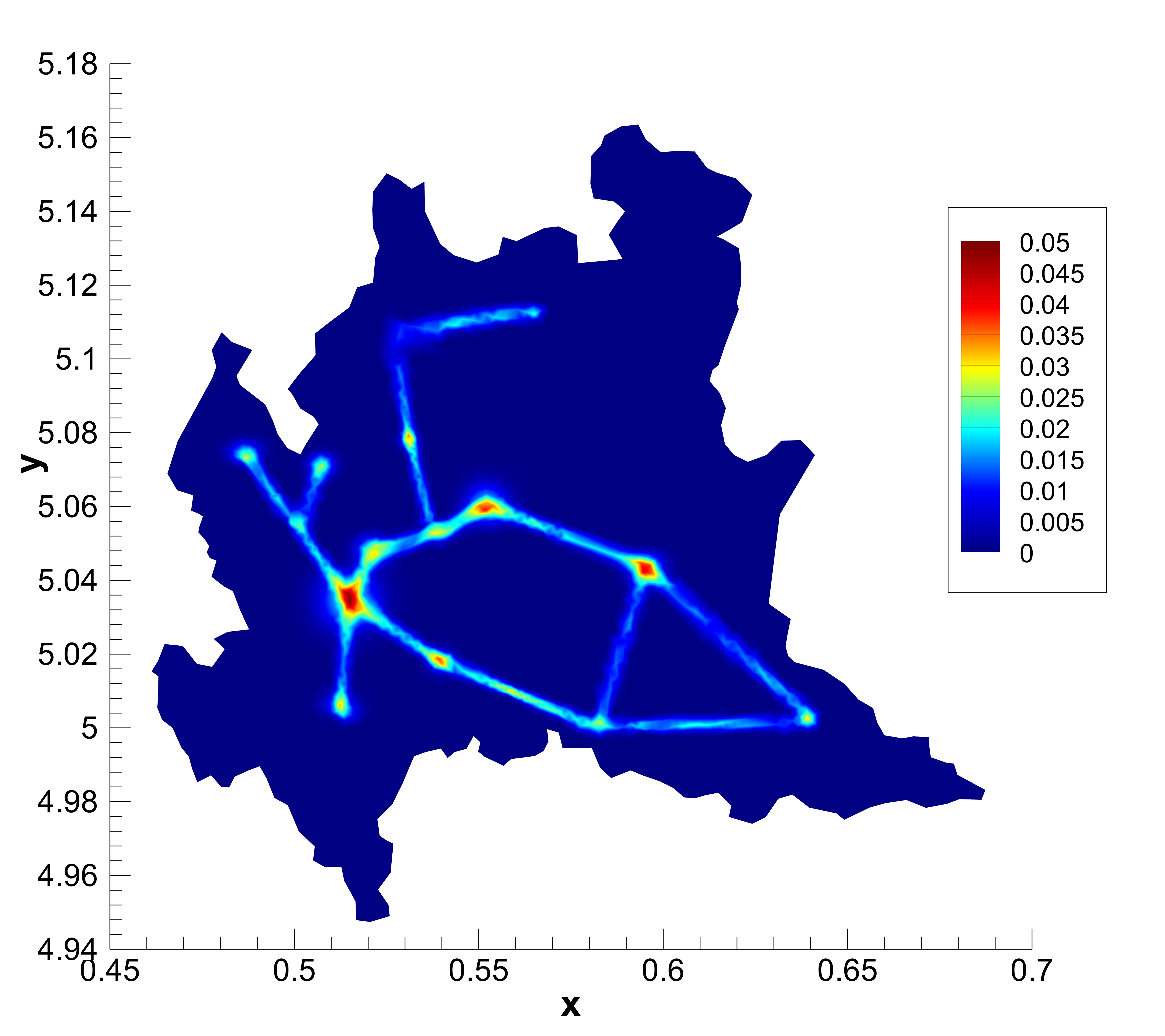
To avoid the mobility of the population in the entire territory and to simulate a more realistic geographical scenario in which individuals travel along the main traffic paths of the Region, different values of propagation speeds are assigned in the domain which reflect, as close as possible, the real characteristics of the territory. Along the main connections of the Region, a mean value of $\lambda=0.04$ is prescribed for compartments $S,E,A$ and $R$, which ensures a maximum travel distance of 80 km within a day; while, for the same compartments, $\lambda=0.02$ is ulterior fixed in the urbanized circles. A spatial width of $h=0.5$ km is assigned to the traveling paths. On the other hand, assuming that highly infectious subjects are mostly detected in the most optimistic scenario, being subsequently quarantined or hospitalized, the speed assigned to compartment $I$ is set null. However, the infected people, even if limited by quarantines and social distancing, can still contribute to the spread the disease via the diffusion process at the urban scale (mimicking for instance the still possible infections happening at the family level). A null value $\lambda=0$ is set in the rest of the computational domain for all the epidemiological compartments. The resulting distribution of the characteristic speeds is visible from Figure 1(c).

The relaxation time is set $\tau_{i}=10^{4}$ for $i\in\{S,E,I,A,R\}$, so that the model recovers a hyperbolic regime in the entire region, apart from the main cities, where a parabolic setting is prescribed to correctly capture the diffusive behavior of the disease spreading which typically occurs in highly urbanized zones. Hence, in the urban area of each city the following relaxation time $\tau_{c,i}$ is prescribed:

$$\tau_{c,i}=\tau_{i}+(\tau_{0}-\tau_{i})\sum_{c=1}^{\mathcal{N}_{c}}e^{-\frac{(x-x_{c})^{2}+(y-y_{c})^{2}}{2r_{c}^{2}}},$$

with a diffusive relaxation time chosen to be $\tau_{0}=10^{-4}$. The resulting distribution of the relaxation times is presented in Figure 1(d).

Considering $p_{c}$ the number of citizens of a generic city (province) denoted with subscript $c$, the initial spatial distribution of the generic population $f(x,y)$ is assigned, for each province and each epidemiological compartment, as a multivariate Gaussian function with the variance being the radius of the urban area $r_{c}$:

$$f(x,y)=\frac{1}{2\pi r_{c}}e^{-\frac{(x-x_{c})^{2}+(y-y_{c})^{2}}{2r_{c}^{2}}}p_{c}\,,$$

with $(x_{c},y_{c})$ representing the coordinates of a generic city center. The initial population setting, for each province of the Lombardy Region, is taken from [63] and reported in Table 1, Appendix A.2. Note that, the radius $r_{c}$ associated to each city, defined in Table 1 (first column), permits to exactly re-obtain the population $p_{c}$ when integrating over the computational domain the initial spatially distributed population.

Since at the beginning of the pandemic, tracking of positive individuals in Italy was very scarce, in this numerical test we consider that the initial amount of infected people is the leading quantity affected by uncertainty. To this aim, we introduce a single source of uncertainty $z$ having uniform distribution, $z\sim\mathcal{U}(0,1)$ so that the initial conditions for compartment $I$, in each control volume, are prescribed as

$$I_{T}(0,z)=I_{T,0}(1+\mu z)\,,$$

with $I_{T,0}$ initial amount of highly infectious corresponding to the values reported by February 27, 2020 in the GitHub repository [64] daily updated by the Civil Protection Department of Italy for each city, listed in the last column of Table 1. This choice effectively associates all infected individuals detected with the $I$ compartment, as a result of the screening policy adopted during February–March 2020 in Italy. In fact, tests to assess the presence of SARS-CoV-2 were performed almost exclusively on patients with consistent symptoms and fever at the beginning of this pandemic. Regarding the uncertainty of these data, we impose $\mu=1$, assuming that at least half of the actual highly symptomatic infected were detected at the beginning of the pandemic outbreak. For all the cities with zero infected detected by February 27, 2020 (e.g., Mantua, Varese, Como and Lecco), we choose to fix $I_{T,0}=1$ in order to assign an effective uncertainty.

Based on the estimations reported in [10], the expected initial amount of exposed $E_{T,0}$ and asymptomatic/mildly symptomatic individuals $A_{T,0}$ is imposed so that $E_{T,0}=10\,I_{T,0}$ and $A_{T,0}=9\,I_{T,0}$ in each location. Therefore, also initial conditions for compartments $E$, $A$ and $S$ become stochastic, depending on the initial amount of severe infectious at each location:

$$E_{T}(0,z)=10\,I_{T}(0,z)\,,\qquad A_{T}(0,z)=9\,I_{T}(0,z)\,,$$

$$S_{T}(0,z)=N-E_{T}(0,z)-I_{T}(0,z)-A_{T}(0,z)\,.$$

Finally, removed individuals are initially set null everywhere in the network, $R_{T}(0,z)=0.0$.

To properly subdivide the population in commuters and non-commuters, regional mobility data are considered. In particular, the matrix of commuters presented in Table 2, Appendix A.2, reflects mobility data provided by the Lombardy Region for the regional fluxes of year 2020 [65], which is in agreement with the one derived from ISTAT data released in October, 2011, as also confirmed in [33]. Therefore, to each control volume, the total percentage of commuters referred to the province where it is located is assigned, and non-commuting individuals are computed as a result of conservation principles. From Table 2 it can be noticed that some connections are not taken into account simply because the amount of commuters along these routes is negligible if compared to the amount of individuals traveling in the other paths and with respect to the dimension of the populations.

Concerning epidemiological parameters, accordingly with values reported in [33, 15, 10], we set $\gamma_{I}\penalty\ =\penalty\ 1/14$, $\gamma_{A}=2\gamma_{I}=1/7$, $a=1/3$, considering these parameters as clinical ones and therefore deterministic. We also assume the probability rate of developing severe symptoms $\sigma=1/12.5$, as in [15, 10].

From the first day simulated in this test, the population was aware of the risk associated with COVID-19 and recommendations such as washing hands often, not touching their faces, avoiding handshakes and keeping distances had already been disseminated by the government, hence, we initially fix coefficients $k_{I}=k_{A}=50$.

The initial value of the transmission rate of asymptomatic/mildly infectious people is calibrated as the result of a least square problem with respect to the observed cumulative number of infected $I_{T}(t)$, through a deterministic SEIAR ODE model set up for the whole Lombardy Region, which provide the estimate $\beta_{A}=0.58\times 10^{-3}$. As previously mentioned, since we are assuming that highly infectious subjects are mostly detected in the most optimistic scenario, being subsequently quarantined or hospitalized, the transmission rate of $I$ is set $\beta_{I}=0.03\,\beta_{A}$, as in [33, 15, 10]. Finally, in the incidence function we fix $p=1$.

With this parametric setup, we obtain an initial expected value of the basic reproduction number for the Region, evaluated as from definition (10), $R_{0}(0)\penalty\ =\penalty\ 3.2$, which is in agreement with estimations reported in [33, 15, 56, 10]. Nevertheless, with the proposed methodology it is possible to present the heterogeneity underlying the basic reproduction number at the local scale, as shown in Figure 2 for $\mu=0$, together with the initial global amount of infected people $E_{T,0}(x,y)+I_{T,0}(x,y)+A_{T,0}(x,y)$ present in the domain.

To model the effects of the lockdown imposed by the government from March 9, 2020 in north of Italy [61], from that day the transmission rate $\beta_{A}$ is reduced by 50%, also increasing the coefficients $k_{I}=k_{A}=80$ as a result of the population becoming increasingly aware of the epidemic risks. In addition, the percentage of commuting individuals is reduced by 60% for each compartment according to mobility data tracked through GPS systems of mobile phones and made temporarily available by Google [1, 56].

Numerical results of the test are reported in Figures 3–7. In Figure 3, the expected evolution in time of the infected individuals, together with 95% confidence intervals, is shown for exposed $E$, highly symptomatic subjects $I$ and asymptomatic or weakly symptomatic people $A$, for each city of the Lombardy Region. Here it is already appreciable the heterogeneity of the diffusion of the virus. Indeed, from the different y-axis scales adopted for the plot of the provinces, it can be noticed that Milan, Bergamo and Brescia present a consistently higher contagion.

From Figure 4 it can be observed that the lower bound of the confidence interval of the cumulative amount in time of highly symptomatic individuals is in line with data reported by the Civil Protection Department of Italy [64]. As expected, due to the uncertainty taken into account, the mean value of the numerical result in each city is higher than the registered one.

The comparison between the expected evolution in time of the cumulative amount of severe infectious with respect to the effective cumulative amount of total infectious people, including asymptomatic and mildly symptomatic individuals, is shown in Figure 5. From this figure it is clear that the number of infections recorded during the first outbreak of COVID-19 in Lombardy represents a clear underestimation of the actual trend of infection suffered by the Region and by Italy as a whole, and how the presence of asymptomatic subjects, not detected, has affected the pandemic evolution.

Numerical results presented in terms of integrated variables for the whole Lombardy are shown in Figure 6, together with the expected temporal evolution of the reproduction number $R_{0}(t)$, again with 95% confidence bands. It is here highlighted that the drop of $R_{0}(t)$ on March 9 reflects the imposition of lockdown restrictions, as presented in the previous Section. Moreover, in this plot, results are reported starting from February 28, instead of February 27, to permit to the system to achieve a correct initialization of the commuters (who are totally placed in the origin location at the beginning of the simulation) during the first day simulated.

In Figure 7, final expectation and variance of the cumulative amount of infected people, namely $E_{T}+A_{T}+I_{T}$, are reported in the 2D framework (first row). If comparing Figure 7(a) with 2(a), it can be noticed that, at the end of March, the virus is no longer majorly affecting the province of Lodi and Cremona, but has been spread arriving to hit most of all Brescia, Milan and Bergamo. Finally, in the second row of Figure 7, the expectation of the susceptible population $S_{T}$ on the initial day simulated (February 27, 2020) is compared with the one obtained at the end of the simulation (March 22, 2020). Here it can be verified that the majority of the population does not leave their home city, as per real behavior, but there is only a small percentage of commuters who move within the domain, along the prescribed routes. Similar results are obtained for compartments $E$ and $A$, whose commuting part, even though small, strongly contributes to the spatial spread of the epidemic.

References

- [1] A. Aktay, S. Bavadekar, G. Cossoul, J. Davis, D. Desfontaines, A. Fabrikant, E. Gabrilovich, K. Gadepalli, B. Gipson, M. Guevara, C. Kamath, M. Kansal, A. Lange, C. Mandayam, A. Oplinger, C. Pluntke, T. Roessler, A. Schlosberg, T. Shekel, S. Vispute, M. Vu, G. Wellenius, B. Williams, and R. J. Wilson. Google COVID-19 Community Mobility Reports: Anonymization Process Description (version 1.1). Preprint arXiv:2004.04145, (2020).
- [2] G. Albi, L. Pareschi, M. Zanella. Control with uncertain data of socially structured compartmental epidemic models. J. Math. Bio. to appear, preprint arXiv:2004.13067, (2020).
- [3] G. Albi, L. Pareschi, M. Zanella. Modelling lockdown measures in epidemic outbreaks using selective socio-economic containment with uncertainty. Preprint medRxiv doi: 10.1101/2020.05.12.20099721, (2020).
- [4] L.J.S. Allen, B.M. Bolker, Y. Lou, A.L. Nevai. Asymptotic profiles of the steady states for an SIS epidemic reaction–diffusion model. Discrete Contin. Dyn. Syst. 21, 1–20, (2008).
- [5] B.N. Ashraf, Economic impact of government interventions during the COVID-19 pandemic: International evidence from financial markets. J. Behav. and Experiment. Finance, 27, 100371, (2020).
- [6] D. Balcan, B. Gonçalves, H. Hu, J.J. Ramasco, V. Colizza, A. Vespignani. Modeling the spatial spread of infectious diseases: the GLobal Epidemic and Mobility computational model. J. Comput. Sci. 1(3):132–145, (2010).
- [7] E. Barbera, G. Consolo, G. Valenti. Spread of infectious diseases in a hyperbolic reaction-diffusion susceptible-infected-recovered model. Phys. Rev. E, 88, 052719 (2013).
- [8] N. Bellomo, R. Bingham, M. A. J. Chaplain, G. Dosi, G. Forni, D. A. Knopoff, J. Lowengrub, R. Twarock, and M. E. Virgillito. A multi-scale model of virus pandemic: Heterogeneous interactive entities in a globally connected world. Math. Mod. & Meth. in Appl. Scie., 30(8):1591–1651, (2020).
- [9] G. Bertaglia, L. Pareschi. Hyperbolic models for the spread of epidemics on networks: kinetic description and numerical methods, ESAIM Math. Model. & Numer. Anal. 55:381–407, (2020).
- [10] G. Bertaglia, L. Pareschi. Hyperbolic compartmental models for epidemic spread on networks with uncertain data: application to the emergence of Covid-19 in Italy. Preprint arXiv:2105.14258, (2021).
- [11] S. Boscarino, L. Pareschi, G. Russo. Implicit-Explicit Runge-Kutta schemes for hyperbolic systems and kinetic equations in the diffusion limit. SIAM J. Sci. Comp. 35:22–51, (2013).
- [12] S. Boscarino, L. Pareschi, G. Russo. A unified IMEX Runge-Kutta approach for hyperbolic systems with multiscale relaxation. SIAM J. Numer. Anal. 55(4):2085–2109, (2017).
- [13] W. Boscheri, G. Dimarco. High order central WENO-Implicit-Explicit Runge Kutta schemes for the BGK model on general polygonal meshes. J. Comp. Phys., 422:109766 (2020).
- [14] W. Boscheri, G. Dimarco, L. Pareschi. Modeling and simulating the spatial spread of an epidemic through multiscale kinetic transport equations. Math. Mod. & Meth. App. Math., to appear (2021).
- [15] B. Buonomo and R. Della Marca. Effects of information-induced behavioural changes during the COVID-19 lockdowns: The case of Italy: COVID-19 lockdowns and behavioral change. Royal Society Open Science, 7(10), (2020).
- [16] K.M. Case, P.F. Zweifel. Existence and Uniqueness Theorems for the Neutron Transport Equation. J. Math. Physics 4(11):1376–1385, (1963).
- [17] V. Capasso. Global solution for a diffusive nonlinear deterministic epidemic model. SIAM J. Appl. Math. 35:274–284, (1978).
- [18] V. Capasso, G. Serio, A generalization of the Kermack-McKendrick deterministic epidemic model. Math. Biosci. 42, 43 (1978).
- [19] C. Cercignani, R. Illner, M. Pulvirenti. The Mathematical Theory of Diluted Gases Springer, New York, (1994).
- [20] F.A.C.C. Chalub, P.A. Markovich, B. Perthame, C. Schmeiser. Kinetic models for chemotaxis and their drift-diffusion limits. Monatsh. Math. 142, 123–141 (2004).
- [21] V. Colizza, A. Vespignani. A. Epidemic modeling in metapopulation systems with heterogeneous coupling pattern: Theory and simulations. J. Theor. Biol. 251:450–467, (2008).
- [22] R.M. Colombo, M. Garavello, F. Marcellini, E. Rossi. An age and space structured SIR model describing the COVID-19 pandemic. J. Math. Ind., 10(1): 22, (2020).
- [23] M. Delitala. Generalized kinetic theory approach to modeling spread- and evolution of epidemics. Math. and Comp. Model., 39(1):1–12, (2004).
- [24] O. Diekmann, J. Heesterbeek, M. Roberts, The construction of next-generation matrices for compartmental epidemic models. J. Roy. Soc. Interface, 7:873–885, (2010).
- [25] G. Dimarco, L. Pareschi. Numerical methods for kinetic equations. Acta Numer. 23:369–520, (2014).
- [26] G. Dimarco, L. Pareschi, G. Toscani, M. Zanella. Wealth distribution under the spread of infectious diseases. Phys. Rev. E, 102, 022303, (2020).
- [27] M. Dumbser, W. Boscheri, M. Semplice, G. Russo. Central weighted ENO schemes for hyperbolic conservation laws on fixed and moving unstructured meshes. SIAM J. Sci. Comp., 39: A2564-A2591 (2017).
- [28] M. Dumbser, M. Kaeser. Arbitrary high order non-oscillatory finite volume schemes on unstructured meshes for linear hyperbolic systems. J. Comp. Phys., 221:693–723 (2007).
- [29] W. E. Fitzgibbon, J. J. Morgan, G. F. Webb. An outbreak vector-host epidemic model with spatial structure: the 2015–2016 Zika outbreak in Rio De Janeiro. Theor. Biol. Med. Model. 14: 7, (2017).
- [30] E. Franco. A feedback SIR (fSIR) model highlights advantages and limitations of infection-based social distancing. Preprint arXiv:2004.13216, (2020).
- [31] E. Frias-Martinez, G. Williamson, V. Frias-Martinez. An Agent-Based Model of Epidemic Spread using Human Mobility and Social Network Information. In Proceedings of the 3rd International Conference on Social Computing (SocialCom11), Boston, MA, USA, 49–56, (2011).
- [32] E. Gaburro, W. Boscheri, S. Chiocchetti, C. Klingenberg, V. Springel, M. Dumbser. High order direct Arbitrary-Lagrangian-Eulerian schemes on moving Voronoi meshes with topology changes. Journal of Computational Physics, 407:109167 (2020).
- [33] M. Gatto, E. Bertuzzo, L. Mari, S. Miccoli, L. Carraro, R. Casagrandi, A. Rinaldo. Spread and dynamics of the COVID-19 epidemic in Italy: Effects of emergency containment measures. Proceed. Nat. Acad. Scie., 117(19):10484–10491, (2020).
- [34] G. Giordano, F. Blanchini, R. Bruno, P. Colaneri, A. Di Filippo, A. Di Matteo, and M. Colaneri. Modelling the COVID-19 epidemic and implementation of populationwide interventions in Italy. Nature Medicine, 26(6):855-860, (2020).
- [35] F. Golse, S. Jin, C. Levermore. The convergence of numerical transfer schemes in diffusive regimes I: Discrete-ordinate method. SIAM J. Num. Anal., 36(5):1333–1369, (1999).
- [36] T. Hillen, A. Swan. The diffusion limit of transport equations in biology. In: Preziosi L., Chaplain M., Pugliese A. (eds) Mathematical Models and Methods for Living Systems. Lect. Notes in Math. 2167, Springer, Cham, (2016).
- [37] H.W. Hethcote, The Mathematics of Infectious Diseases. SIAM Review 42(4):599–653, (2000).
- [38] S. Jin, H. Lu, L. Pareschi. Efficient stochastic asymptotic-preserving implicit-explicit methods for transport equations with diffusive scalings and random inputs. SIAM J. Sci. Comput. 40(2):A671–A696, (2018).
- [39] S. Jin, L. Pareschi, G. Toscani. Uniformly accurate diffusive relaxation schemes for multiscale transport equations. SIAM J. Num. Anal., 38(3):913–936, (2000).
- [40] J.P. Keller, L. Gerardo-Giorda, A. Veneziani. Numerical simulation of a susceptible-exposed-infectious space-continuous model for the spread of rabies in raccoons across a realistic landscape. J. Biol. Dyn., 7(1):31–46, (2014).
- [41] A. Klar, An asymptotic-induced scheme for nonstationary transport equations in the diffusive limit. SIAM J. Numer. Anal., 35, 1073–1094, (1998).
- [42] A. Korobeinikov, P. K. Maini. Non-linear incidence and stability of infectious disease models. Math. Med. and Bio.: A Journal of the IMA, 22, 113–128, (2005).
- [43] E.W. Larsen, J.B. Keller. Asymptotic solution of neutron transport problems for small free mean paths. J. Math. Phys., 15:75–81, (1974).
- [44] E. Loli Piccolomini and F. Zama. Monitoring Italian COVID-19 spread by a forced SEIRD model. PloS one, 15(8):e0237417, (2020).
- [45] Q-X. Liu, Z. Jin. Formation of spatial patterns in an epidemic model with constant removal rate of the infectives. J. Stat. Mech.: Theory and Experiment, 2007(05):P05002–P05002,(2007).
- [46] P. Magal, G.F. Webb, X. Wu. Spatial spread of epidemic diseases in geographical settings: Seasonal influenza epidemics in Puerto Rico. Discr. & Cont. Dyn. Sys. - B,25(6):2185–2202, (2019).
- [47] B. Perthame. Transport Equations in Biology. Birkhäuser, Boston, (2007)
- [48] L. Pareschi and G. Toscani. Interacting multiagent systems: kinetic equations and Monte Carlo methods, Oxford University Press, Oxford, UK, (2014).
- [49] M. Peirlinck, K. Linka, F. Sahli Costabal, J. Bhattacharya, E. Bendavid, J. P. Ioannidis, and E. Kuhl. Visualizing the invisible: The effect of asymptomatic transmission on the outbreak dynamics of COVID-19. Comp. Meth. in Appl. Mech. and Eng., 372(1):113410, (2020).
- [50] M. Pulvirenti, S. Simonella. A kinetic model for epidemic spread. Math. Mech. Complex Systems, 8(3):249–260, (2020).
- [51] S. Riley, K. Eames, V. Isham, D. Mollison, P. Trapman. Five challenges for spatial epidemic models. Epidemics, 10:68–71, (2015).
- [52] G. Sun. Pattern formation of an epidemic model with diffusion. Nonlinear Dyn. 69:1097–1104, (2012).
- [53] B. Tang, X. Wang, A. Li, N.L. Bragazzi, S. Tang, Y. Xiao, J. Wu. Estimation of the transmission risk of the 2019-nCoV and its implication for public health interventions. J. Clinical Med. 9, 462 (2020).
- [54] A. Viguerie, G. Lorenzo, F. Auricchio, D. Baroli, T.J.R. Hughes, A. Patton, A. Reali, T.E. Yankeelov, A. Veneziani. Simulating the spread of COVID-19 via a spatially-resolved susceptible–exposed–infected–recovered–deceased (SEIRD) model with heterogeneous diffusion. Appl. Math. Letters, 101:106617, (2021).
- [55] A. Viguerie, A. Veneziani, G. Lorenzo, D. Baroli, N. Aretz-Nellesen, A. Patton, T.E. Yankeelov, A. Reali,T.J.R. Hughes, F. Auricchio. Diffusion–reaction compartmental models formulated in a continuum mechanics framework: application to COVID-19, mathematical analysis, and numerical study. Comput. Mech., 66, 1131–1152, (2020).
- [56] M. A. C. Vollmer, S. Mishra, H. J. T. Unwin, A. Gandy, T. A. Mellan, H. Zhu, H. Coupland, I. Hawryluk, M. Hutchinson, O. Ratmann, P. Walker, C. Whittaker, L. Cattarino, C. Ciavarella, L. Cilloni, M. Baguelin, S. Bhatia, A. Boonyasiri, N. Brazeau, G. Charles, V. Cooper, Z. Cucunuba, G. Cuomo-dannenburg, A. Dighe, B. Djaafara, J. Eaton, L. V. Elsland, R. Fitzjohn, K. Fraser, K. Gaythorpe, W. Green, S. Hayes, N. Imai, E. Knock, D. Laydon, J. Lees, T. Mangal, A. Mousa, G. Nedjati-gilani, P. Nouvellet, D. Olivera, K. V. Parag, M. Pickles, H. A. Thompson, R. Verity, H. Wang, Y. Wang, O. J. Watson, L. Whittles, X. Xi, and A. Ghani. Using mobility to estimate the transmission intensity of COVID-19 in Italy: a subnational analysis with future scenarios. Technical Report May, Imperial College London, (2020).
- [57] G.F. Webb. A reaction-diffusion model for a deterministic diffusion epidemic. J. Math. Anal. Appl., 84: 150–161, (1981).
- [58] J. Wang, F. Xie, T. Kuniya. Analysis of a reaction-diffusion cholera epidemic model in a spatially heterogeneous environment. Comm. Nonlin. Sci. and Num. Simul., 80:104951, (2020).
- [59] R. Yano. Kinetic modeling of local epidemic spread and its simulation. J. Sci. Comput., 73:122–156, (2017).
- [60] D. Xiu, Numerical Methods for Stochastic Computations: A Spectral Method Approach. Princeton University Press, Princeton, NY (2010).
- [61] Chronology of main steps and legal acts taken by the Italian Government for the containment of the COVID-19 epidemiological emergency. (http://www.protezionecivile.gov.it/documents/20182/1227694/Summary+of+\\measures+taken+against+the+spread+of+C-19/c16459ad-4e52-4e90-90f3-\\c6a2b30c17eb)
- [62] Istituto Nazionale di Statistica, Italia. Dati Geografici, (https://www4.istat.it/it/archivio/209722)
- [63] Istituto Nazionale di Statistica, Italia. Dati Demografici, (http://demo.istat.it/)
- [64] Presidenza del Consiglio dei Ministri, Dipartimento della Protezione Civile, Italia. COVID-19 epidemiological data in Italy, (https://github.com/pcm-dpc/COVID-19)
- [65] Regione Lombardia, Italia. Open Data, (https://www.dati.lombardia.it/Mobilit-e-trasporti/Matrice-OD2020-Passeggeri/hyqr-mpe2)