跳到论文正文
W Papers独立论文阅读器 arXiv:2106.07142 论文正文 计算阅读时间 · 0%
引用这篇论文根据当前论文元数据生成,正式投稿前建议核对。


License: arXiv.org perpetual non-exclusive license
arXiv:2106.07142v2 [math.CO] 20 Sep 2022

Planarity in Generalized Scattering Amplitudes: PK Polytope, Generalized Root Systems and Worldsheet AssociahedraThanks: Perimeter Institute for Theoretical Physics and the Institute for Advanced Study.
email: earlnick@ias.edu

Nick Early
Abstract.

In this paper we study the role of planarity in generalized scattering amplitudes, through several closely interacting structures in combinatorics, algebraic and tropical geometry.

The generalized biadjoint scalar amplitude, introduced recently by Cachazo-Early-Guevara-Mizera (CEGM), is a rational function of homogeneous degree −(k−1)​(n−k−1)-(k-1)(n-k-1) in (nk)−n\binom{n}{k}-n independent variables, calculated by summing over all solutions of the generalized scattering equations; its poles are in bijection with coarsest positroidal subdivisions of the hypersimplex Δk,n\Delta_{k,n} and can be constructed directly from the rays of the positive tropical Grassmannian.

We introduce for each pair of integers (k,n)(k,n) with 2≤k≤n−22\leq k\leq n-2 a system of generalized positive roots which arises as a specialization of the planar basis of kinematic invariants. We prove that the higher root polytope ℛn−k(k)\mathcal{R}^{(k)}_{n-k} has volume Cn−k(k)C^{(k)}_{n-k} by exhibiting a flag unimodular triangulation into simplices, in bijection with noncrossing collections of (k−1)​(n−k−1)(k-1)(n-k-1) kk-element subsets of {1,…,n}\{1,\ldots,n\}. Here Cn−k(k)C^{(k)}_{n-k} is the kk-dimensional Catalan number, which counts for instance the number of standard rectangular Young tableaux. As an application of our results for generalized roots, we give a bijection between certain positroidal subdivisions of the hypersimplex Δ3,n\Delta_{3,n}, which we call tripods, and the set of noncrossing pairs of 3-element subsets that are not weakly separated.

We show that the facets of the Planar Kinematics (PK) polytope, introduced recently by Cachazo and the author, are exactly the (nk)−n\binom{n}{k}-n generalized positive roots. We show that the PK specialization of the generalized biadjoint amplitude evaluates to Cn−k(k)C^{(k)}_{n-k}.

Looking forward, we give defining equations, and conjecture explicit solutions using the space (ℂ​ℙn−k−1)×(k−1)(\mathbb{CP}^{n-k-1})^{\times(k-1)} via a notion of compatibility degree for noncrossing collections, for a two parameter family of generalized worldsheet associahedra 𝒲k,n+\mathcal{W}^{+}_{k,n}. These specialize when k=2k=2 to the dihedrally invariant partial compactification of the configuration space M0,nM_{0,n} of nn distinct points in ℂ​ℙ1\mathbb{CP}^{1}. Many detailed examples are given throughout to motivate future work.

1. Introduction

In 1948, Richard Feynman introduced a pictorial formalism in Quantum Field Theory (QFT) to organize the expansion of scattering amplitudes as sums of elementary building blocks, labeled by graphs. These graphs, now called Feynman diagrams, specify which singularities of the amplitude are compatible and can be reached simultaneously.

In [21], Cachazo, Early Guevara and Mizera (CEGM) introduced higher analog of scattering equations, and a higher analog of the biadjoint scalar partial amplitude mn(2)(=mnCLOSEm^{(2)}_{n}(=m_{n}, in the usual notation). In the higher analog, the (k,n)(k,n) generalized biadjoint amplitude mn(k)m^{(k)}_{n} acts as an interpolation between nn copies of mn−1(k−1)m^{(k-1)}_{n-1} and nn copies of mn−1(k)m^{(k)}_{n-1}. There is a generalized notion of Feynman diagrams for the theory, given by collections of Feynman diagrams [9] and [30] as well as [22], and parametrized by arrangements of metric trees on certain boundaries of a polytope. The singularities of mn(k)m^{(k)}_{n} are extremely complex. Each of these is a hyperplane defined by the vanishing of some linear function of Mandelstam parameters 𝔰J\mathfrak{s}_{J}, but the decomposition is not unique and does not provide much intuition. Therefore it would be very helpful to have an efficient and compact way to organize them. They key idea is to look at subdivisions of convex polytopes called hypersimplices Δk,n\Delta_{k,n} which arise in combinatorial geometry. In the case at hand, one considers those subdivisions which are regular: they are induced by projecting down the facets in the lower envelope of the convex hull of lifted vertices of Δk,n\Delta_{k,n}. A particular kind of tropical hypersurface, called a blade [28], plays a special role here. The standard blade ((,,,,,,,))((1,2,\ldots,n)), pinned to vertices of Δk,n\Delta_{k,n}, induces a basis of (nk)−n\binom{n}{k}-n kinematic functions ηJ​(𝔰)\eta_{J}(\mathfrak{s}) such that ηJ​(𝔰)=0\eta_{J}(\mathfrak{s})=0 characterizes a pole of mn(k)m^{(k)}_{n}. Moreover, other poles possess particularly simple expansions as integer linear combination of the ηJ​(𝔰)\eta_{J}(\mathfrak{s})’s. Then mn(k)m^{(k)}_{n} becomes a (finite) sum of simple rational functions which have distinct nonzero iterated residues, where each denominator factor is dual to a weighted blade arrangement [31].

Returning to CEGM amplitudes mn(k)m^{(k)}_{n}: they have an extremely rich structure and the classification poses a significant challenge11 1 Still it could be worse! Poles of the CEGM scattering equations formula for mn(k)m^{(k)}_{n} are known [7] to be in bijection with coarsest regular positroidal subdivisions, which are actually well-behaved in the wider context of all regular matroid subdivisions of Δk,n\Delta_{k,n}, that is the full Dressian Drk,n\text{Dr}_{k,n}.. A key item on the wishlist is a fully detailed and constructive description of the residues of mn(k)m^{(k)}_{n}, but this has been considered completely unattainable in any generality. One problem is that coarsest regular positroidal subdivisions of Δk,n\Delta_{k,n} have (so far, at least) resisted classification; another source of difficulty seems intriguing: there is a rich structure of linear dependencies among the residues which arises from non-simplicial cones in the secondary fan, the positive tropical Grassmannian Trop+​G​(k,n)\text{Trop}^{+}G(k,n). One could in principle try to resolve such linear dependencies, by enlarging the kinematic space and triangulating the maximal cones in Trop+​G​(k,n)\text{Trop}^{+}G(k,n). This could be implemented in practice by for instance including certain higher degree polynomials in the Plucker coordinates into the CEGM potential, such as those coming directly from the cluster algebra of the Grassmannian. This in itself seems like a difficult and potentially interesting problem; but we take a different route. Instead of enlarging the CEGM potential, we deform it to something that is extremely well-behaved.

Thus, the purpose of this work is to construct a deformation mn(k),N​Cm^{(k),NC}_{n} of mn(k)m^{(k)}_{n} which is possible to describe in complete generality. More precisely, we deform the Plucker coordinates pJp_{J} on G⁡(k,n)G(k,n) with certain Laurent polynomials. After fixing a parametrization, these Laurent polynomials become multi-homogeneous polynomials τJ​(xi,j)\tau_{J}(x_{i,j}) for (i,j)∈[1,k−1]×[1,n−k](i,j)\in[1,k-1]\times[1,n-k]. We are interested in the Newton polytope of the product ∏JτJ\prod_{J}\tau_{J}; we conjecture a combinatorial formula for its face lattice. Our deformation mn(k),N​Cm^{(k),NC}_{n} is at the very least a rich testing ground for properties of CEGM amplitudes, but seems interesting in its own right from the perspective of algebraic, convex, combinatorial and tropical geometry.

We study the k=3k=3 case mn(3),N​Cm^{(3),NC}_{n} in depth and formulate a conjecture which leads to an all (k,n) formula for the rational function expansion of mn(k),N​Cm^{(k),NC}_{n} as a sum of reciprocals of products of simple linear functions in (nk)−n\binom{n}{k}-n independent parameters, and we obtain supporting evidence for our formula for large values of (k,n)(k,n); on the other hand, the analogous calculation CEGM amplitudes seems far out of reach.

In parallel, we construct a triangulation of a generalization of the type AA root polytope, defined in [23], denoted ℛn(k)\mathcal{R}^{(k)}_{n}, which is the convex hull of a set of generalized positive roots which live in the Cartesian product of k−1k-1 root systems of type An−k−1A_{n-k-1}. We exhibit an explicit triangulation of ℛn(k)\mathcal{R}^{(k)}_{n} and show that the complex of simplices in the triangulation is isomorphic to the (reduced) noncrossing complex 𝐍𝐂k,n\mathbf{NC}_{k,n}. In particular this means that ℛn(k)\mathcal{R}^{(k)}_{n} has volume the kk-dimensional Catalan number Cn−k(k)C^{(k)}_{n-k}, where for example Cn−2(2)=2,5,14,42,…C^{(2)}_{n-2}=2,5,14,42,\ldots for n=4,5,6,7,…n=4,5,6,7,\ldots and Cn−3(3)=5,42,462,6006,…,C^{(3)}_{n-3}=5,42,462,6006,\ldots, for n=5,6,7,8,…n=5,6,7,8,\ldots. Here 𝐍𝐂k,n\mathbf{NC}_{k,n} was studied by Petersen, Pylyavskyy and Speyer in [49] and in for instance the work of Santos, Stump and Welker in [56] on the so-called Grassmann associahedron22 2 Here the noncrossing complex 𝐍𝐂k,n\mathbf{NC}_{k,n} was denoted Δ~k,nN​C\tilde{\Delta}^{NC}_{k,n}. We change notation to avoid conflict with the hypersimplex.. Then the noncrossing triangulation of ℛn(k)\mathcal{R}^{(k)}_{n} should be dual to the Grassmann associahedron. Our main conjecture makes this duality explicit.

We finally initiate the systematic study of generalized positive roots, in the context of the poset of cones in the positive tropical Grassmannian Trop+​G​(k,n)\text{Trop}^{+}G(k,n). In particular, generalized positive roots and the noncrossing complex provides a rich framework to explore the poset of cones in Trop+​G​(k,n)\text{Trop}^{+}G(k,n), and to explore the poset of regular positroidal subdivisions of Δk,n\Delta_{k,n}.

1.1. Outline of the rest of the Introduction

In this paper, we have included an extended introduction whose aim is to articulate and motivate our objectives for a diverse audience. The structure is as follows.

  1. (1)

    Section 1.2 gives a concise summary of our main results, and Section 1.3 contains an outline of the paper.

  2. (2)

    Section 1.4 contains key definitions and notations. In particular it has the definition of the noncrossing complex 𝐍𝐂k,n\mathbf{NC}_{k,n}.

  3. (3)

    Section 1.5 formulates the question we consider from a physical point of view and then motivates our strategy through constructions in combinatorial geometry.

1.2. Background and Summary of Results

In [21], Cachazo, Guevara, Mizera and the author (CEGM) introduced a generalization of the Cachazo-He-Yuan (CHY) definition of biadjoint double partial amplitudes mn​(𝕀,𝕀)m_{n}(\mathbb{I},\mathbb{I}) where 𝕀=(12⋯n)\mathbb{I}=(12\cdots n) is the standard cyclic order, from integrals over the moduli space of nn points on ℂ​ℙ1\mathbb{CP}^{1} modulo projective equivalence, localized to points satisfying the scattering equations [15, 16, 17, 32], to integrals over the space

X⁡(k,n)={g∈G⁡(k,n):∏JpJ≠0}/(ℂ∗)nX(k,n)=\left\{g\in G(k,n):\prod_{J}p_{J}\not=0\right\}\big/\penalty(\mathbb{C}^{\ast})^{n}

localized to solutions of the generalized scattering equations. Here pJp_{J} is a Plucker coordinate, the k×kk\times k determinant with column set JJ.

In 2013, CHY [17] solved the scattering equations for a special choice of kinematics, via a high-energy limit of the type A1A_{1} Y-system, proving analytically, by summing all ⌊(n−1)/2⌋\lfloor(n-1)/2\rfloor solutions to the Planar Kinematics scattering equations, that the biadjoint partial amplitude evaluates to the Catalan number33 3 Note that we follow the convention of the original paper of CHY [17], where there is an alternating sign.

mn​(𝕀,𝕀)=(−1)n+1​Cn−2(2)m_{n}(\mathbb{I},\mathbb{I})=(-1)^{n+1}C^{(2)}_{n-2}

where

Cn−2(2)=2,5,14,42,132,…C^{(2)}_{n-2}=2,5,14,42,132,\ldots

with n=4,5,6,7,8,…n=4,5,6,7,8,\ldots the 2-dimensional Catalan numbers.

The generalized biadjoint partial amplitude mn(k)​(𝕀,𝕀)m^{(k)}_{n}(\mathbb{I},\mathbb{I}) is a highly structured rational function m(k)​(𝕀n,𝕀n)m^{(k)}(\mathbb{I}_{n},\mathbb{I}_{n}) on a dimension (nk)−n\binom{n}{k}-n kinematic space 𝒦⁡(k,n)\mathcal{K}(k,n); it is calculated by summing over the critical points of the potential function

(1) 𝒮k,n\displaystyle\mathcal{S}_{k,n} =\displaystyle= ∑1≤j1<⋯<jk≤nlog(pj1,…,jk)sj1⋯jk,\displaystyle\sum_{1\leq j_{1}<\cdots<j_{k}\leq n}\log(p_{j_{1},\ldots,j_{k}})s_{j_{1}\cdots j_{k}},

where sj1⋯jks_{j_{1}\cdots j_{k}} are parameters with distinct (unordered) indices. It grows quickly in size and complexity as kk increases. The poles alone can be as complicated as any coarsest regular positroidal subdivision of the hypersimplex Δk,n\Delta_{k,n}, see [9, 22, 29, 31, 44, 59, 8] and have as such resisted attempts to make a systematic classification.

In this paper, we study a polytope which is defined from Equation (1) at the special kinematic point, the Planar Kinematics (PK) point. With respect to the cyclic order (12⋯n)(12\cdots n), the PK point is given by

s12​…​k=s23​…​k+1=…=sn​1​…​k−1\displaystyle s_{12\ldots k}=s_{23\ldots k+1}=\ldots=s_{n1\ldots k-1} =\displaystyle= 1,\displaystyle 1,
sn​1​…​k−2,k=s12​…​k−1,k+1=…=sn−1,n​…​k−3,k−1\displaystyle s_{n1\ldots k-2,k}=s_{12\ldots k-1,k+1}=\ldots=s_{n-1,n\ldots k-3,k-1} =\displaystyle= −1,\displaystyle-1,

where all other sJs_{J} are set to zero. The PK point has an equivalent characterization in terms of the planar basis of linear functions ηJ\eta_{J} on the kinematic space 𝒦⁡(k,n)⊂ℝ(nk)\mathcal{K}(k,n)\subset\mathbb{R}^{\binom{n}{k}}, wherein all ηJ\eta_{J} are set to 1. This basis was introduced in [17] for k=2k=2 and subsequently generalized to all kk in [30, 31]. The planar kinematics scattering equations appear as the set of equations occurring as the first derivatives of the PK potential function

𝒮k,n(P​K)=∑j=1nlog⁡(pj,j+1,…,j+k−2,j+k−1pj,j+1,…,j+k−2,j+k),\mathcal{S}^{(PK)}_{k,n}=\sum_{j=1}^{n}\log\left(\frac{p_{j,j+1,\ldots,j+k-2,j+k-1}}{p_{j,j+1,\ldots,j+k-2,j+k}}\right),

which provides a (ℂ∗)n(\mathbb{C}^{\ast})^{n}-invariant analog of the mirror superpotential [53, 54], see also [39],

ℱq:=∑i=1,i≠n−knpi,i+1,…,i+(k−2),i+kpi,i+1,…,i+(k−2),i+(k−1)+q​pn−k,n−k+1,…,n−1,1pn−k,n−k+1,…,n−1,n.\displaystyle{\mathcal{F}}_{q}:=\sum_{i=1,\,i\neq n-k}^{n}\frac{p_{i,i+1,\ldots,i+(k-2),i+k}}{p_{i,i+1,\ldots,i+(k-2),i+(k-1)}}+q\frac{p_{n-k,n-k+1,\ldots,n-1,1}}{p_{n-k,n-k+1,\ldots,n-1,n}}.

In [24], the PK potential function 𝒮k,n(P​K)\mathcal{S}^{(PK)}_{k,n} was defined as a specialization of the potential function arising in the generalized scattering equations [21]. Here the main result was to prove that critical points of 𝒮k,n(P​K)\mathcal{S}^{(PK)}_{k,n} lift to (equivalence classes of) critical points of ℱq\mathcal{F}_{q}.

In more detail, it was shown that the critical points of 𝒮k,n(P​K)\mathcal{S}^{(PK)}_{k,n} can be represented by images of certain kk-tuples of roots of unity which inject via the Veronese mapping into the torus quotient G⁡(k,n)/(ℂ∗)nG(k,n)/\penalty(\mathbb{C}^{\ast})^{n}. Specifically, the injection is from the set of kk-tuples of roots of unity which do not sum to zero, into the set of binary Lyndon words with kk ones and n−kn-k zeros. The critical points of the PK potential function are equivalence classes of those critical points of the mirror superpotential studied in [53] and [54], coming from kk-tuples or roots of unity which do not sum to zero.

In this paper, we study the PK potential function in its own right; in [24] Cachazo and the author introduced the Planar Kinematics (PK) polytope Πn−k(k)\Pi^{(k)}_{n-k}, which is the convex hull of all exponent vectors of monomials appearing in exp⁡(−𝒮k,n(P​K))\exp\left(-\mathcal{S}^{(PK)}_{k,n}\right) under a certain parameterization. More precisely, we need that

exp⁡(−𝒮k,n(P​K))=∏j=1npj,j+1,…,j+k−2,j+kpj,j+1,…,j+k−2,j+k−1\exp\left(-\mathcal{S}^{(PK)}_{k,n}\right)=\prod_{j=1}^{n}\frac{p_{j,j+1,\ldots,j+k-2,j+k}}{p_{j,j+1,\ldots,j+k-2,j+k-1}}

becomes a Laurent polynomial when it is evaluated on the image of the positive parameterization [1] of the nonnegative Grassmannian; see Section 7 below for a Newton-polytopal reinterpretation. Based on that finding44 4 Note the departure from [24], Πn−k(k)\Pi^{(k)}_{n-k} was defined in terms of facet inequalities; in this paper we prove that the latter is equal to the Newton polytope here., we make the definition

(2) Πn−k(k)=Newt​(P1⋯Pk−1Q1⋯Qn−k−1∏(i,j)∈[1,k−1]×[1,n−k]xi,j),\displaystyle\Pi^{(k)}_{n-k}=\text{Newt}\left(\frac{P_{1}\cdots P_{k-1}Q_{1}\cdots Q_{n-k-1}}{\prod_{(i,j)\in[1,k-1]\times[1,n-k]}x_{i,j}}\right),

where

Pi=∑j=1n−kxi,j,P_{i}=\sum_{j=1}^{n-k}x_{i,j},

whose Newton polytope is a simplex of dimension n−k−1n-k-1,

Newt​(Pi)={∑j=1n−kαi,j​ei,j:∑j=1n−kαi,j=1},\text{Newt}(P_{i})=\left\{\sum_{j=1}^{n-k}\alpha_{i,j}e_{i,j}:\sum_{j=1}^{n-k}\alpha_{i,j}=1\right\},

and where

Qj=∑{(ti)∈{0,1}k−1:t1≤⋯≤tk−1}x1,j+t1x2,j+t2⋯xk−1,j+tk−1Q_{j}=\sum_{\{(t_{i})\in\{0,1\}^{k-1}:\ t_{1}\leq\cdots\leq t_{k-1}\}}x_{1,j+t_{1}}x_{2,j+t_{2}}\cdots x_{k-1,j+t_{k-1}}

has Newton polytope

Newt(Qj)={∑i=1k−1αi,jei,j+αi,j+1ei,j+1:1≥α1,j≥α2,j≥⋯≥αk−1,j≥0,αi,j+αi,j+1=1},\text{Newt}(Q_{j})=\left\{\sum_{i=1}^{k-1}\alpha_{i,j}e_{i,j}+\alpha_{i,j+1}e_{i,j+1}:1\geq\alpha_{1,j}\geq\alpha_{2,j}\geq\cdots\geq\alpha_{k-1,j}\geq 0,\ \alpha_{i,j}+\alpha_{i,j+1}=1\right\},

a simplex of dimension k−1k-1.

Our approach this paper to study Πn−k(k)\Pi^{(k)}_{n-k} relies on a generalization [24] of the system of positive roots of type AA is embedded in a (k−1)(k-1)-fold Cartesian product of root lattices of type Dynkin type An−kA_{n-k}. We observe that the set of linear dependencies for this lattice of higher roots is governed by noncrossing combinatorics of kk-element sets; we prove that the higher rank root polytope ℛn−k(k)\mathcal{R}^{(k)}_{n-k}, admits a unimodular triangulation into Cn−k(k)C^{(k)}_{n-k} simplices of maximal dimension (k−1)​(n−k−1)(k-1)(n-k-1), where Cn−k(k)C^{(k)}_{n-k} is a kk-dimensional Catalan number, which counts for instance the number of rectangular k×nk\times n standard Young tableaux:

k∖nk\setminus n 44 55 66 77 88
22 22 55 1414 4242 132132
33 55 4242 462462 6 0066\,006
44 1414 462462 24 02424\,024
55 4242 6 0066\,006
66 132132

.

Let us first recall from [24] the construction of higher positive roots, that is to say the linear functions γJ\gamma_{J}, defined as follows. Let ei,je_{i,j} be the standard basis for ℝ(k−1)×(n−k)\mathbb{R}^{(k-1)\times(n-k)} with coordinate functions αi,j\alpha_{i,j}. For any subset JJ of {1,…,n}\{1,\ldots,n\} define αi,J=∑t∈Jαi,t\alpha_{i,J}=\sum_{t\in J}\alpha_{i,t}. When J=∅J=\emptyset then αi,∅=0\alpha_{i,\emptyset}=0.

Now for each kk-element subset JJ of {1,…,n}\{1,\ldots,n\}, denote by γJ:ℝ(k−1)×(n−k)→ℝ\gamma_{J}:\mathbb{R}^{(k-1)\times(n-k)}\rightarrow\mathbb{R} the generalized root

(3) γJ​(α)=∑i=1k−1αi,[ji−(i−1),ji+1−i−1].\displaystyle\gamma_{J}(\alpha)=\sum_{i=1}^{k-1}\alpha_{i,[j_{i}-(i-1),j_{i+1}-i-1]}.

Choosing new variables αi,j′\alpha^{\prime}_{i,j} such that αi,j=αi,t′−αi,t+1′\alpha_{i,j}=\alpha^{\prime}_{i,t}-\alpha^{\prime}_{i,t+1}, for each i=1,…,k−1i=1,\ldots,k-1 we recover one copy of the usual system of positive roots αi,a′−αi,b′\alpha^{\prime}_{i,a}-\alpha^{\prime}_{i,b} for a<ba<b.

Note that γJ\gamma_{J} is identically zero when JJ is a subinterval J=[i,i+(k−1)]J=[i,i+(k-1)] of {1,…,n}\{1,\ldots,n\}. Usually we omit the argument of γJ​(α)\gamma_{J}(\alpha) and write simply γJ\gamma_{J}.

Given a k−1k-1 tuple of integers λ=(λ1,…,λk−1)\mathbf{\lambda}=(\lambda_{1},\ldots,\lambda_{k-1}), denote by ℋk,nλ\mathcal{H}^{\lambda}_{k,n} the codimension (k−1)(k-1) (affine) subspace of ℝ(k−1)×(n−k)\mathbb{R}^{(k-1)\times(n-k)},

(4) ℋk,nλ\displaystyle\mathcal{H}^{\lambda}_{k,n} =\displaystyle= {(α)∈ℝ(k−1)×(n−k):∑j=1n−kαi,j=λi,i=1,…,k−1}.\displaystyle\left\{(\alpha)\in\mathbb{R}^{(k-1)\times(n-k)}:\sum_{j=1}^{n-k}\alpha_{i,j}=\lambda_{i},\ i=1,\ldots,k-1\right\}.

When λ=(0,…,0)\lambda=(0,\ldots,0) we write just ℋk,n\mathcal{H}_{k,n}.

Denote by ℛ^n−k(k)\hat{\mathcal{R}}^{(k)}_{n-k} the root polytope, the convex hull of the linear functions γJ\gamma_{J},

ℛ^n−k(k)=convex hull​({0}∪{γJ:J∈([n]k)})\hat{\mathcal{R}}^{(k)}_{n-k}=\text{convex hull}\left(\{0\}\cup\left\{\gamma_{J}:J\in\binom{[n]}{k}\right\}\right)

and by ℛn−k(k)\mathcal{R}^{(k)}_{n-k} its dimension (k−1)​(n−k−1)(k-1)(n-k-1) projection, which is the convex hull of the restricted functions

ℛn−k(k)=convex hull​{γJ|ℋk,n:J∈([n]k)n​f}.\mathcal{R}^{(k)}_{n-k}=\text{convex hull}\left\{\gamma_{J}|_{\mathcal{H}_{k,n}}:J\in\binom{[n]}{k}^{nf}\right\}.

Our main result for the PK polytope is the explicit set of (irredundant) facet inequalities.

Theorem 1.1.

We have

(5) Πn−k(k)\displaystyle\Pi^{(k)}_{n-k} =\displaystyle= {(α)∈ℝ(k−1)×(n−k):∑j=1n−kαi,j=0;γJ(α)+1≥0,J∈([n]k)n​f}\displaystyle\left\{(\alpha)\in\mathbb{R}^{(k-1)\times(n-k)}:\sum_{j=1}^{n-k}\alpha_{i,j}=0;\ \gamma_{J}(\alpha)+1\geq 0,\ J\in\binom{[n]}{k}^{nf}\right\}

and each inequality defines a facet.

In particular it turns out that Πn−k(k)\Pi^{(k)}_{n-k} lives in the intersection of a codimension k−1k-1 subspace of ℝ(k−1)×(n−k)\mathbb{R}^{(k-1)\times(n-k)} with the cube [−1,2](k−1)×(n−k)[-1,2]^{(k-1)\times(n-k)}.

Our main result for the root polytope ℛn−k(k)\mathcal{R}^{(k)}_{n-k} is that it admits a triangulation which is governed by the complex of pairwise noncrossing collections of kk-element subsets 𝐍𝐂k,n\mathbf{NC}_{k,n}, see Definition 1.9. This generalizes the result due [34], for the triangulation of the root polytope, the convex hull of the positive roots ei−eje_{i}-e_{j} together with the origin, using certain alternating trees. See also [50], and [43].

For any collection 𝒥={J1,…,Jm}∈𝐍𝐂k,n\mathcal{J}=\{J_{1},\ldots,J_{m}\}\in\mathbf{NC}_{k,n} of nonfrozen subsets JiJ_{i}, define

[𝒥]\displaystyle[\mathcal{J}] =\displaystyle= Convex hull​({0,γJ1,…,γJm})\displaystyle\text{Convex hull}(\left\{0,\gamma_{J_{1}},\ldots,\gamma_{J_{m}}\right\})
Theorem 1.2.

The set of simplices {[𝒥]:𝒥∈𝐍𝐂k,n}\left\{[\mathcal{J}]:\mathcal{J}\in\mathbf{NC}_{k,n}\right\} defines a flag, unimodular triangulation55 5 A triangulation is flag if it is the clique complex of its 1-skeleton: every complete subgraph of the 1-skeleton is the 1-skeleton of a simplex in the triangulation. A triangulation is unimodular if every (maximal dimension) simplex has the same volume 1d!\frac{1}{d!}, where dd is the dimension. of ℛn−k(k)\mathcal{R}^{(k)}_{n-k}.

We formulate a conjectural formula for the resolved biadjoint scalar m^n(3),N​C​(𝕀,𝕀)\hat{m}^{(3),NC}_{n}(\mathbb{I},\mathbb{I}) which also uses the noncrossing complex.

For any 1≤i<j<k≤n1\leq i<j<k\leq n, define a compound determinant

Ai​j​k=det((u1×u2)×(ui×ui+1),uj,(uj+1×uj+2)×(uk×u1)),A_{ijk}=\det\left((u_{1}\times u_{2})\times(u_{i}\times u_{i+1}),u_{j},(u_{j+1}\times u_{j+2})\times(u_{k}\times u_{1})\right),

for a given matrix with columns u1,…,un∈ℂ3u_{1},\ldots,u_{n}\in\mathbb{C}^{3}.

For each 2≤j<k≤n2\leq j<k\leq n define

p^1​j​k=p1​j​k,\hat{p}_{1jk}=p_{1jk},

while for 2≤i<j<k≤n2\leq i<j<k\leq n define the resolved minor

p^i​j​k=Ai​j​kp1,2,i+1​p1,j+1,j+2\hat{p}_{ijk}=\frac{A_{ijk}}{p_{1,2,i+1}p_{1,j+1,j+2}}

and the resolved potential function

𝒮^3,n=∑1≤i<j<k≤nlog⁡(p^i​j​k)​si​j​k\hat{\mathcal{S}}_{3,n}=\sum_{1\leq i<j<k\leq n}\log(\hat{p}_{ijk})s_{ijk}

Finally, denote by m^n(3),N​C​(𝕀,𝕀)\hat{m}^{(3),NC}_{n}(\mathbb{I},\mathbb{I}) the resolved amplitude

m^n(3),N​C​(𝕀,𝕀)=∑(x)∈critical points​(𝒮^3,n​(s))1det′Φ⁡(x)​∏j=1n(1p^j,j+1,j+2​(x))2,\hat{m}^{(3),NC}_{n}(\mathbb{I},\mathbb{I})=\sum_{(x)\in\text{critical points}(\hat{\mathcal{S}}_{3,n}(s))}\frac{1}{\det^{\prime}\Phi(x)}\prod_{j=1}^{n}\left(\frac{1}{\hat{p}_{j,j+1,j+2}(x)}\right)^{2},

where det′Φ\det^{\prime}\Phi is the so-called reduced Hessian determinant (see [21, Equation 2.4] for details) of 𝒮^3,n\hat{\mathcal{S}}_{3,n}. See also [19] for general results, and [64] for a reformulation using the Euler operator.

Conjecture 1.3.

There exists a set of linear functions η^J​(s)\hat{\eta}_{J}(s) such that

(6) m^n(3),N​C​(𝕀,𝕀)=∑{J1,…,J(2)​(n−4)}∈𝐍𝐂3,n∏j=1(2)​(n−4)1η^Jj.\displaystyle\hat{m}^{(3),NC}_{n}(\mathbb{I},\mathbb{I})=\sum_{\{J_{1},\ldots,J_{(2)(n-4)}\}\in\mathbf{NC}_{3,n}}\prod_{j=1}^{(2)(n-4)}\frac{1}{\hat{\eta}_{J_{j}}}.

See Appendix B for a detailed, numerical calculation for large prime-number kinematics in the case (k,n)=(3,6)(k,n)=(3,6).

A formula for the resolved planar kinematic functions η^J\hat{\eta}_{J} is conjectured in Equation (70).

Next, we define variables, generalized cross-ratios ui​j​ku_{ijk}, which can be extended via the positive parameterization (see Section 7 for a reinterpretation which is convenient for our purposes) to provide a combinatorial characterization of a compactification of the configuration space of nn generic points in ℂ​ℙ2\mathbb{CP}^{2} modulo projective equivalence; conjecturally the strata in the compactification are in bijection with pairwise noncrossing collections of 33-element subsets of {1,…,n}\{1,\ldots,n\}. It is now natural to propose analogous constructions for all k≥2k\geq 2, which we do, in Section 11.

Planar face polynomials τJ\tau_{J} are defined in Section 6. For each i=2,3,…,ni=2,3,\ldots,n, define τ1,i=1.\tau_{1,i}=1. With integers s≥0s\geq 0 and m≥2m\geq 2, and an mm-element subset J={j1,…,jm}J=\{j_{1},\ldots,j_{m}\} of {2,3,…,n}\{2,3,\ldots,n\}, set

τ(s)J=∑{A∈ℐJ:a1≤a2≤⋯≤am}x1+s,a1x2+s,a2⋯xm+s,am,\tau^{(s)}_{J}=\sum_{\{A\in\mathcal{I}_{J}:a_{1}\leq a_{2}\leq\cdots\leq a_{m}\}}x_{1+s,a_{1}}x_{2+s,a_{2}}\cdots x_{m+s,a_{m}},

where A={a1,…,am}A=\{a_{1},\ldots,a_{m}\}, and

ℐJ=[j1−1,j2−1]×[j2−2,j3−2]×⋯[jm−1−(m−1),jm−m].\mathcal{I}_{J}=[j_{1}-1,j_{2}-1]\times[j_{2}-2,j_{3}-2]\times\cdots[j_{m-1}-(m-1),j_{m}-m].

We are now ready to define the face polynomials τJ\tau_{J}.

Definition 1.4.

For any I∈([n]k)I\in\binom{[n]}{k}, let s≥0s\geq 0 be such that I=[1,s]∪JI=[1,s]\cup J, where J=I∖[1,s]J=I\setminus[1,s]. Now define

τI=τj1−s,j2−s,…,jm−s(s).\tau_{I}=\tau^{(s)}_{j_{1}-s,j_{2}-s,\ldots,j_{m}-s}.

Here [1,0]=∅[1,0]=\emptyset is the empty set.

Note that the τJ\tau_{J} polynomials are not irreducible in general.

Figure 1. The Staircase: the (irreducible) Planar Face polynomial τ2,6,11,12,14\tau_{2,6,11,12,14}.

Then for instance for k=3k=3 we have τ1,2,j=1\tau_{1,2,j}=1 for all j=3,…,nj=3,\ldots,n. For {1,j,k}\{1,j,k\} such that 3≤j<k≤n3\leq j<k\leq n, then

τ1,j,k\displaystyle\tau_{1,j,k} :⁣=\displaystyle:= ∑a∈[j−1,k−2]x2,a.\displaystyle\sum_{a\in[j-1,k-2]}x_{2,a}.

Whenever {i,j,k}\{i,j,k\} satisfies 2≤i≤j<k≤n2\leq i\leq j<k\leq n, then

τi,j,k\displaystyle\tau_{i,j,k} :⁣=\displaystyle:= ∑{(a,b)∈[i−1,j−1]×[j−2,k−3],a≤b}x1,a​x2,b\displaystyle\sum_{\{(a,b)\in[i-1,j-1]\times[j-2,k-3],\ a\leq b\}}x_{1,a}x_{2,b}

We finally define the u-variables for k=3k=3 and then formulate the main conjecture.

For any {i,j,k}⊂{1,…,n}\{i,j,k\}\subset\{1,\ldots,n\} that is not one of the nn cyclic intervals {j,j+1,j+2}\{j,j+1,j+2\}, define

ui,j,k​(x)={τi,n−1,nτi−1,n−1,n,(i,j,k)=(i,n−1,n)τi+1,j,k​τi,j+1,j+2τi,j,k​τi+1,j+1,j+2,j+1<k,k=n,τi+1,j,k​τi,j,k+1τi,j,k​τi+1,j,k+1,k<n.\displaystyle u_{i,j,k}(x)=\begin{cases}\frac{\tau_{i,n-1,n}}{\tau_{i-1,n-1,n}},&(i,j,k)=(i,n-1,n)\\ \frac{\tau_{i+1,j,k}\tau_{i,j+1,j+2}}{\tau_{i,j,k}\tau_{i+1,j+1,j+2}},&j+1<k,\ \ k=n,\\ \frac{\tau_{i+1,j,k}\tau_{i,j,k+1}}{\tau_{i,j,k}\tau_{i+1,j,k+1}},&k<n.\end{cases}

When it is clear from context, we will abbreviate ui​j​k​(x)u_{ijk}(x) with just ui​j​ku_{ijk}.

Conjecture 1.5.

For any J∈([n]3)n​fJ\in\binom{[n]}{3}^{nf}, we have

(7) uJ\displaystyle u_{J} =\displaystyle= 1−∏{I:(I,J)∉𝐍𝐂3,n}ucI,JI,\displaystyle 1-\prod_{\{I:\ (I,J)\not\in\mathbf{NC}_{3,n}\}}u^{c_{I,J}}_{I},

where for any crossing pair (i1​i2​i3,j1​j2​j3)∉𝐍𝐂3,n(i_{1}i_{2}i_{3},j_{1}j_{2}j_{3})\not\in\mathbf{NC}_{3,n},

(8) c(i1,i2,i3),(j1,j2,j3)={2if ​i1<j1<i2<j2<i3<j3​ or ​j1<i1<j2<i2<j3<i31otherwise.\displaystyle c_{(i_{1},i_{2},i_{3}),(j_{1},j_{2},j_{3})}=\begin{cases}2&\text{if }i_{1}<j_{1}<i_{2}<j_{2}<i_{3}<j_{3}\text{ or }j_{1}<i_{1}<j_{2}<i_{2}<j_{3}<i_{3}\\ 1&\text{otherwise}.\end{cases}

We have confirmed explicitly that Equations (7) and (8) hold for u-variables of type (3,n)(3,n) for all n≤15n\leq 15. For k=4k=4, the u-variables are defined explicitly in Equation (53).

In Definition 11.4 (reproduced below) we formulate the all-(k,n) definition of the generalized worldsheet. It is not difficult to see that it recovers the case k=3k=3 above, as well as the dihedral compactification studied in [14] and [5] in the case k=2k=2. These all provide examples of positive geometries [4]. We also conjecture a parameterization of the solution space, given explicitly in the cases 3,43,4 with k≥5k\geq 5 straightforward to infer. It would be very interesting to find a combinatorial proof that our parameterization solves the binary equations below!

For any I,J∈(nk)n​fI,J\in\binom{n}{k}^{nf}, the compatibility degree cI,Jc_{I,J} is the number of violations of the noncrossing condition in the pair (I,J)(I,J). Let us be more precise.

Definition 1.6.

Given I,J∈(nk)n​fI,J\in\binom{n}{k}^{nf}, then the compatibility degree cI,J≥0c_{I,J}\geq 0 is the number of pairs ({i1,i2},{j1,j2})(\{i_{1},i_{2}\},\{j_{1},j_{2}\}) with {ia,ib}⊆I\{i_{a},i_{b}\}\subseteq I and {jc,jd}⊆J\{j_{c},j_{d}\}\subseteq J, such that (ia,ib),(jc,jd)(i_{a},i_{b}),(j_{c},j_{d}) is not weakly separated and we are in either of the following situations: b=a+1b=a+1 and d=c+1d=c+1 or iℓ=jℓi_{\ell}=j_{\ell} for each ℓ=a+1,a+2,…,b−1\ell=a+1,a+2,\ldots,b-1.

Definition 1.7.

The generalized worldsheet associahedron 𝒲k,n+\mathcal{W}^{+}_{k,n} is the set of all points (uJ)∈[0,1](nk)−n(u_{J})\in[0,1]^{\binom{n}{k}-n} such that the following set of equations hold: for each J∈([n]k)n​fJ\in\binom{[n]}{k}^{nf}, one equation

(9) uJ\displaystyle u_{J} =\displaystyle= 1−∏{I:(I,J)∉𝐍𝐂k,n}ucI,JI,\displaystyle 1-\prod_{\{I:\ (I,J)\not\in\mathbf{NC}_{k,n}\}}u^{c_{I,J}}_{I},

where cI,Jc_{I,J} is the compatibility degree from Definition 11.3.

Conjecture 1.8.

Equations (54) generate the ideal of relations among the planar face ratios uJ​(τ)u_{J}(\tau).

Finally, Root Kinematics, and the Root Kinematics potential function 𝒮k,n(R​t)\mathcal{S}^{(Rt)}_{k,n}, are formulated in Definition 8.2, where it is shown that, in a precise sense, it induces a non-recursive construction of the positive parameterization of G⁡(k,n)/(ℂ∗)nG(k,n)/\penalty(\mathbb{C}^{\ast})^{n}, as the solution to a differential equation; however it requires a nontrivial amount of machinery to do properly and it would not make sense to repeat the discussion here in the Introduction. Nonetheless we can extract the key piece: 𝒮k,n(R​t)\mathcal{S}^{(Rt)}_{k,n} can be reconstituted from its value on the positive parameterization66 6 We use the notation BCFW, after the recursion of Britto-Cachazo-Feng-Witten [10]; see [1] for further discussion. of the nonnegative Grassmannian [51, 65] (Section 7). This value is:

(10) 𝒮k,n(R​t)|B​C​F​W\displaystyle\mathcal{S}^{(Rt)}_{k,n}\big|_{BCFW} =\displaystyle= ∑(i,j)∈[1,k−1]×[1,n−k]log⁡(xi,j∑ℓ=1n−kxi,ℓ)​αi,j,\displaystyle\sum_{(i,j)\in[1,k-1]\times[1,n-k]}\log\left(\frac{x_{i,j}}{\sum_{\ell=1}^{n-k}x_{i,\ell}}\right)\alpha_{i,j},

where xi,jx_{i,j} are homogeneous coordinates on (ℂ​ℙn−k−1)×(k−1)(\mathbb{CP}^{n-k-1})^{\times(k-1)}.

1.3. Structure of the rest of the paper

The paper is structured as follows.

  • •

    Section 1.4 contains key notation and conventions, as well as an extended discussion of motivation.

  • •

    Sections 3 and 4 contain our main result for the higher root polytopes ℛn−k(k)\mathcal{R}^{(k)}_{n-k}, namely that they admit a flag unimodular triangulation into simplices in bijection with noncrossing collections in 𝐍𝐂k,n\mathbf{NC}_{k,n}.

  • •

    Section 5 studies the use of the planar kinematic invariants ηJ\eta_{J} as height functions over the vertices of root polytopes. For k=2k=2 it works perfectly in that it induces the noncrossing triangulation; however for k≥3k\geq 3 some subtle issues emerge.

  • •

    Section 6 defines the Planar Kinematics (PK) associahedron 𝕂n−k(k)\mathbb{K}^{(k)}_{n-k}, of which the PK polytope is a Minkowski subsummand.

  • •

    Section 7 reinterprets the matrix entries of the positive parameterization in terms of Newton polytopes.

  • •

    Section 8 builds on the earlier noncrossing triangulation of ℛn−k(k)\mathcal{R}^{(k)}_{n-k} to derive a noncrossing representation of the rays of the positive tropical Grassmannian. In particular, a notion of a noncrossing degree is defined.

  • •

    Section 9 formulates the main ingredients for the k=3k=3 instance of the generalized worldsheet associahedron, 𝒲3,n+\mathcal{W}^{+}_{3,n}, as a compactification of the configuration space of nn generic points in ℂ​ℙ2\mathbb{CP}^{2}.

  • •

    Section 10 brings our PK polytope story to a close, with a complete description of its facets. The proof invokes the noncrossing expansion coming form the complete simplicial fan in Theorem 4.3.

  • •

    In Section 11 we define the generalized worldsheet associahedron 𝒲k,n+\mathcal{W}^{+}_{k,n} for arbitrary (k,n)(k,n), in terms of an explicit set of binary equations, with exponents involving a certain compatibility degree for the noncrossing complex.

  • •

    Appendix A reviews material about blades from previous work.

  • •

    Appendix B includes a numerical evaluation of the resolved amplitude m^n(3),N​C\hat{m}^{(3),NC}_{n} using the generalized scattering equations [21]. This is provides the first consistency check against our formulation of the generalized worldsheet associahedron 𝒲3,n+\mathcal{W}^{+}_{3,n}.

  • •

    Appendix C formulates the k=3k=3 and k=4k=4 planar face ratios and lays the groundwork for the computation of noncrossing binary identities for all kk. In this way, we define for each (k,n)(k,n) a generalized worldsheet associahedron which specializes to the dihedrally invariant partial compactification of the configuration space of nn distinct points in ℂ​ℙ1\mathbb{CP}^{1}, see for instance [40, 55, 11, 5].

1.4. Notation and Key Definitions

Let us first fix some notation.

Set [n]={1,…,n}[n]=\{1,\ldots,n\} and denote by ([n]k)\binom{[n]}{k} the set of kk-element subsets of [n][n]. Call a subset JJ frozen if its indices form a cyclic interval with respect to the cyclic order (12⋯n)(12\cdots n); otherwise it is nonfrozen. Let ([n]k)n​f\binom{[n]}{k}^{nf} be the set of all nonfrozen kk-element subsets of {1,…,n}\{1,\ldots,n\}.

The hypersimplex Δk,n\Delta_{k,n} is the convex polytope

Δk,n={x∈[0,1]n:∑j=1nxj=k}.\Delta_{k,n}=\left\{x\in[0,1]^{n}:\sum_{j=1}^{n}x_{j}=k\right\}.

It is the convex hull of the set of all points in the unit cube [0,1]n[0,1]^{n} with kk ones and n−kn-k zeros.

Given subsets I,J∈([n]k)I,J\in\binom{[n]}{k}, write I≺JI\prec J if II is lexicographically smaller than JJ.

The weak separation condition in Definition 1.9 is due to Leclerc and Zelevinsky in [41]; the formulation of the noncrossing criterion given here is our interpretation of the definition given in [56].

Definition 1.9 ([56]).

A pair I,J∈([n]k)I,J\in\binom{[n]}{k} is said to be weakly separated, with respect to the cyclic order (1,2,…,n)(1,2,\ldots,n), provided that the coordinates in the difference eI−eJe_{I}-e_{J} of vertices eI,eJ∈Δk,ne_{I},e_{J}\in\Delta_{k,n} does not contain the pattern77 7 In the context of [29], the sign pattern avoidance has the direct interpretation that the arrangement of βI,βJ\beta_{I},\beta_{J} of the blade β=((,,,,,,,))\beta=((1,2,\ldots,n)) on the vertices eI,eJ∈Δk,ne_{I},e_{J}\in\Delta_{k,n}, respectively, cuts any octahedral face of Δk,n\Delta_{k,n} at most once, and consequently the subdivision induced in Δk,n\Delta_{k,n} is matroidal, and in particular positroidal. ea−eb+ec−ede_{a}-e_{b}+e_{c}-e_{d} for a<b<c<da<b<c<d, up to cyclic rotation.

A pair I,J∈([n]k)I,J\in\binom{[n]}{k} of kk-element subsets of {1,…,n}\{1,\ldots,n\} is said to be non-crossing, with respect to the linear order 1<2<⋯<n1<2<\cdots<n, provided that for each 1≤a<b≤k1\leq a<b\leq k, then either

  1. (1)

    The pair {{ia,ia+1,…,ib},{ja,ja+1,…,jb}}\{\{i_{a},i_{a+1},\ldots,i_{b}\},\{j_{a},j_{a+1},\ldots,j_{b}\}\} is weakly separated, or

  2. (2)

    The interiors of the respective intervals do not coincide, that is we have

    {ia+1,…,ib−1}≠{ja+1,…,jb−1}.\{i_{a+1},\ldots,i_{b-1}\}\not=\{j_{a+1},\ldots,j_{b-1}\}.

Clearly there is some redundancy above that could be eliminated, but for our purposes this formulation is preferred.

Denote by 𝐖𝐒k,n\mathbf{WS}_{k,n} the poset of all collections of pairwise weakly separated nonfrozen kk-element subsets, ordered by inclusion; according to the purity conjecture for weakly separated collections states that, among these, the maximal (by inclusion) collections of these each have exactly (k−1)​(n−k−1)(k-1)(n-k-1) kk-element subsets. The purity conjecture was proved independently in [26], [47].

Denote by 𝐍𝐂k,n\mathbf{NC}_{k,n} the poset of all collections of pairwise non-crossing nonfrozen k-element subsets, ordered by inclusion; again, it is known that the maximal (by inclusion) collections of these each have exactly (k−1)​(n−k−1)(k-1)(n-k-1) kk-element subsets, see [49], [56].

We emphasize that in our definition of the noncrossing complex 𝐍𝐂k,n\mathbf{NC}_{k,n}, the nn frozen subsets that consist of a single cyclic interval are excluded; sometimes 𝐍𝐂k,n\mathbf{NC}_{k,n} has been called the reduced noncrossing complex, as in for instance [56]. For us, this reduction has in fact it has a physical origin, namely that the generalized biadjoint scalar [21] is a rational function of total degree −(k−1)​(n−k−1)-(k-1)(n-k-1). In particular, the planar kinematic invariants ηJ\eta_{J} with JJ a frozen subset are all identically zero on the kinematic space.

The kinematic space 𝒦⁡(k,n)\mathcal{K}(k,n) is a dimension (nk)−n\binom{n}{k}-n subspace of ℝ(nk)\mathbb{R}^{\binom{n}{k}}, given by

𝒦(k,n)={(s)∈ℝ(nk):∑J∋asJ,a=1,…,n}.\mathcal{K}(k,n)=\left\{(s)\in\mathbb{R}^{\binom{n}{k}}:\sum_{J\ni a}s_{J},\ a=1,\ldots,n\right\}.

Denote by 𝒦D​(k,n)\mathcal{K}_{D}(k,n) the following planar cone inside the kinematic space:

(11) 𝒦D​(k,n)\displaystyle\mathcal{K}_{D}(k,n) =\displaystyle= {(s)∈𝒦(k,n):sJ≤0,J∈([n]k)n​f,sj,j+1,…,j+k−1≥0}.\displaystyle\left\{(s)\in\mathcal{K}(k,n):s_{J}\leq 0,\ J\in\binom{[n]}{k}^{nf},\ s_{j,j+1,\ldots,j+k-1}\geq 0\right\}.

Call a point 𝒦D​(k,n)\mathcal{K}_{D}(k,n) interior if all inequalities are strict. This cone will be used in Section 5 in the construction of certain regular subdivisions of the root polytope ℛn−k(k)\mathcal{R}^{(k)}_{n-k}. The cells in the subdivision form what is called a polyhedral complex.

Definition 1.10.

A polyhedral complex 𝒞\mathcal{C} is a set of polyhedra, such that

  1. (1)

    Every face of a polyhedron from 𝒞\mathcal{C} is also in 𝒞\mathcal{C},

  2. (2)

    The intersection of any two polyhedra C1,C2∈𝒞C_{1},C_{2}\in\mathcal{C} is a face of both C1C_{1} and C2C_{2}.

A polyhedral fan is a polyhedral complex such that every polyhedron is a cone from the origin; it is simplicial if every polyhedron is simplicial. A polyhedral fan 𝒞\mathcal{C} in some ℝm\mathbb{R}^{m} is complete if for any v∈ℝmv\in\mathbb{R}^{m}, then there exists a unique cone C∈𝒞C\in\mathcal{C} such that vv is in the relative interior of CC.

1.5. Motivation

Recent progress in the study of scattering amplitudes digs deep into structures in combinatorial and tropical geometry, revealing two closely related notions of the generalized biadjoint scalar amplitude [21] and stringy integrals [6], both of which – on their common intersection – are governed by degenerations of point configurations in complex projective space that are subject to a certain condition of planarity. The generalized biadjoint scalar amplitude is known to control only the leading order term in the so-called α′\alpha^{\prime}-expansion88 8 Here α′\alpha^{\prime} corresponds in the case k=2k=2 to the so-called inverse string tension. of a stringy integral, but does not suffer from convergence issues and can be calculated in somewhat greater generality.

One immediate lesson is that it may be time to revisit of how physical processes are represented. What should be the correct notion of the worldsheet in the generalization? This is not completely obvious given what is now known as it involves selecting the right compactification of the configuration space X⁡(k,n)X(k,n) of nn generic points in ℂ​ℙk−1\mathbb{CP}^{k-1} modulo P​G​L​(k)PGL(k), where k≥2k\geq 2 is fixed and X⁡(2,n)X(2,n) gives, after a certain planar compactification, the worldsheet for the usual cubic scalar amplitude. In this paper, we formulate the rules for a compactification whose strata are – conjecturally – in bijection with the set of complete subgraphs of the so-called noncrossing complex of kk-element subsets 𝐍𝐂k,n\mathbf{NC}_{k,n}.

One drawback – or, more optimistically, feature – is that our compactification ultimately has to break a cyclic symmetry which was an essential feature for the biadjoint scalar partial amplitude mn(k=2)m^{(k=2)}_{n}, arising from a certain color-order decomposition using structure constants of some gauge group U⁡(N)U(N).

Next, what does it mean for particles to go on-shell in these models which are governed by point configurations in higher dimensional projective spaces? Is the on-shell condition the end of the story for particle interactions? The answer to these questions is manifold and involves an intricate and growing network of connections between algebraic, combinatorial and tropical geometry, the scattering equations formalism and the formulation of stringy integrals. In what follows, we shall refer to both the generalized biadjoint scalar and stringy integrals as instances of generalized scattering amplitudes, though some fundamental physical questions remain to be explored before this designation can be made precise.

According to the blade model [30, 31] for generalized scattering amplitudes [21, 6], planarity is an emergent property of a simple fundamental building block: the simplex, x1≤x2≤⋯≤xn≤x1+1x_{1}\leq x_{2}\leq\cdots\leq x_{n}\leq x_{1}+1. The key player is the normal fan to this simplex, or more precisely the blade ((,,,,,,,))((1,2,\ldots,n)) see [28, 45], which has a certain cyclic symmetry. The prototypical nondegenerate blade ((,,,,,,,))((1,2,\ldots,n)) can be thought of as a discrete curvature; the blade generates physical events, such as when a collection of particles goes on-shell. At first sight the setup of the blade model may seem somewhat too simplistic to describe physical processes; but its flexibility becomes more apparent when it is applied in the context of the biadjoint scalar, using the scattering equations [15, 16], and the subsequent generalization to higher Grassmannians and their compactified torus quotients, [21]. Taking weighted arrangements of ((,,,,,,,))((1,2,\ldots,n)) on the vertices of certain convex polytopes, called hypersimplices Δk,n\Delta_{k,n} and imposing a compatibility condition on octahedral faces of Δk,n\Delta_{k,n} gives rise to matroidal weighted blade arrangements [31], and among these one finds the singularities of these generalized amplitudes.

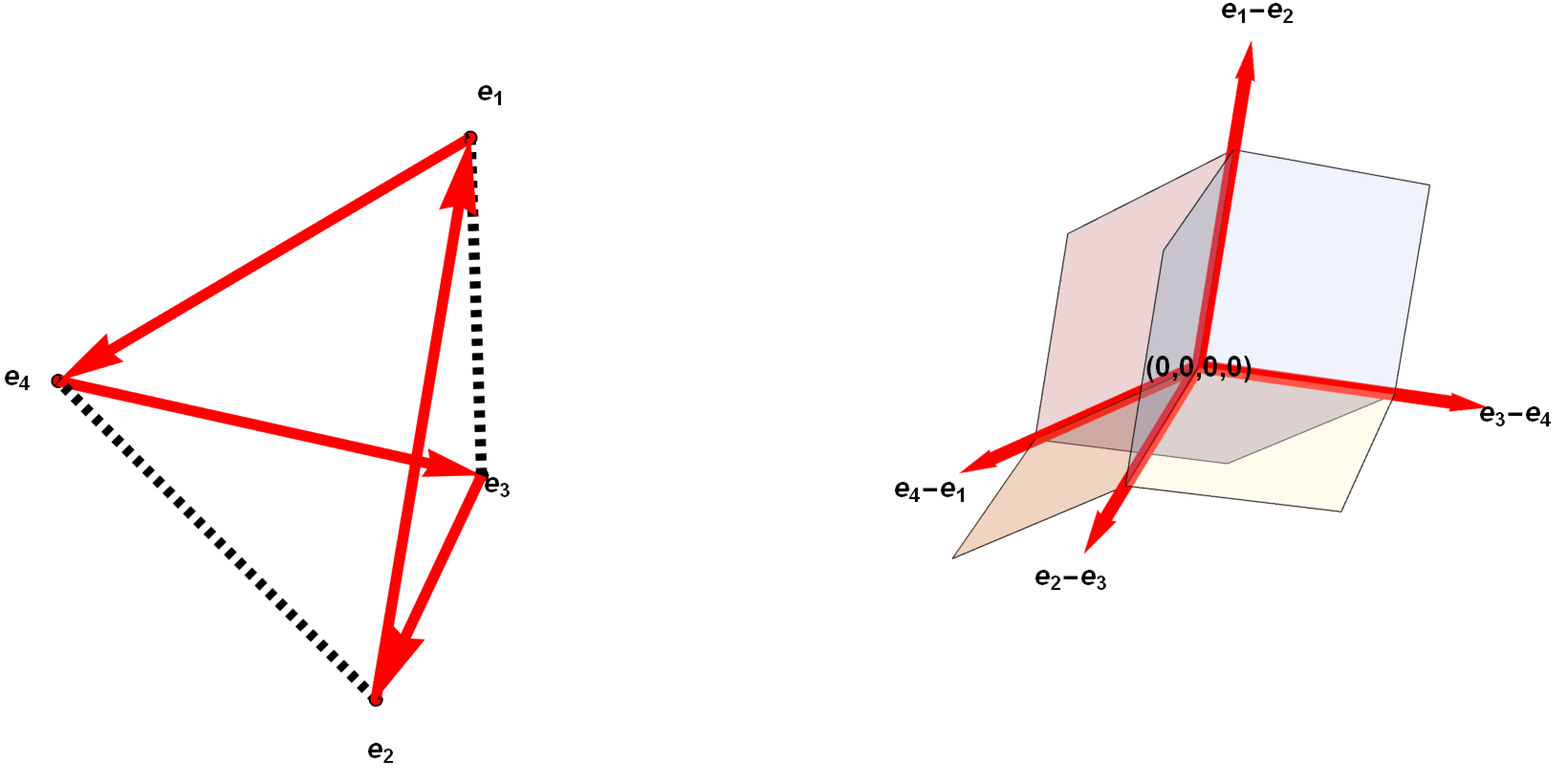
The blade ((,,,,,,,))((1,2,\ldots,n)) is a special kind of tropical hypersurface which induces a decomposition of an n-1 dimensional space into nn chambers, simplicial cones C1,…,CnC_{1},\ldots,C_{n}, where cyclically adjacent pairs intersect in a copy of the simple roots of S​Ln−1SL_{n-1}, more precisely, the intersections of cones Cj∩Cj+1C_{j}\cap C_{j+1} have the n−2n-2 edges ej+1−ej+2,ej+2−ej+3,…,ej−2−ej−1e_{j+1}-e_{j+2},e_{j+2}-e_{j+3},\ldots,e_{j-2}-e_{j-1}, compatibly with the cyclic order (1,…,n)(1,\ldots,n), and the set of all edges ei−ei+1e_{i}-e_{i+1} of the blade sums to zero as in Figure 2.

The relevant question here is how planarity emerges: it emerges for generalized amplitudes through its selection of a preferred planar basis of linear functions on the kinematic space,

ηj1⋯jk=−1n∑I∈([n]k)min{(et+1+2et+2+⋯+(n−1)et−1)⋅(eI−eJ):t=1,…,n}sI,\eta_{j_{1}\cdots j_{k}}=-\frac{1}{n}\sum_{I\in\binom{[n]}{k}}\min\{(e_{t+1}+2e_{t+2}+\cdots+(n-1)e_{t-1})\cdot(e_{I}-e_{J}):t=1,\ldots,n\}s_{I},

which are identified with arrangements of the blade ((,,,,,,,))((1,2,\ldots,n)) on the vertices eJ=∑j∈Jeje_{J}=\sum_{j\in J}e_{j} of Δk,n\Delta_{k,n}. Here J={j1,…,jk}J=\{j_{1},\ldots,j_{k}\}, and the sIs_{I} are coordinate functions on ℝ(nk)\mathbb{R}^{\binom{n}{k}}. The planar basis is in duality with height functions which induce certain matroid subdivisions of the hypersimplex Δk,n\Delta_{k,n}. In case k=2k=2, then one has the remarkable identity

ηi​j=∑i+1≤a<b≤jsa​b,\eta_{ij}=\sum_{i+1\leq a<b\leq j}s_{ab},

where si​js_{ij} are coordinate functions on ℝ(n2)\mathbb{R}^{\binom{n}{2}}. In the case of the cubic scalar theory, one often restricts to the subset of ℝ(n2)\mathbb{R}^{\binom{n}{2}} where si​j=pi⋅pjs_{ij}=p_{i}\cdot p_{j} with respect to the Minkowski bilinear pairing on nn given points in momentum space p1,…,pnp_{1},\ldots,p_{n}, in which case ηi​j=0\eta_{ij}=0 expresses the condition that a cyclically consecutive subset of particles goes on-shell and we have

(pi+1+pi+2+⋯+pj)2=∑i+1≤a<b≤jsa​b=0,(p_{i+1}+p_{i+2}+\cdots+p_{j})^{2}=\sum_{i+1\leq a<b\leq j}s_{ab}=0,

where we will following the usual convention in physics in saying that the si​js_{ij} are called Mandelstam invariants99 9 However, for the purposes of the amplitude one can simply take si,js_{i,j} to be formal parameters, as we do in the rest of this paper.. Note that here as usual pj⋅pj=0p_{j}\cdot p_{j}=0. Due to momentum conservation, such singularities exhibit the usual two-fold symmetry

(12) (pi+1+pi+2+⋯pj)2=(pj+1+pj+2+⋯pi)2.\displaystyle\left(p_{i+1}+p_{i+2}+\cdots p_{j}\right)^{2}=\left(p_{j+1}+p_{j+2}+\cdots p_{i}\right)^{2}.

However, generalized amplitudes are constructed in [21] as a generalization of the so-called biadjoint scalar amplitude using the CHY scattering equations formalism [15], now for all k≥2k\geq 2; now Mandelstam variables are a priori formal parameters si1​…​iks_{i_{1}\ldots i_{k}} indexed by kk distinct, unordered indices, and right away one faces the perplexing situation of a singularity of the generalized amplitude that exhibits behaviors that are a priori unexpected from a physical point of view; the aim of this paper is to answer some of this challenge.

For instance, already for the n=6n=6 point generalized biadjoint scalar amplitude m(3)​(α,β)m^{(3)}(\alpha,\beta) introduced in [21], where we fix the same cyclic order α=β=(1,2,…,6)\alpha=\beta=(1,2,\ldots,6), one has the following three manifestly different ways to write the same pole η1,3,5\eta_{1,3,5}:

(13) η135\displaystyle\eta_{135} =\displaystyle= s123+s126+s136+s234+s235+s236\displaystyle s_{123}+s_{126}+s_{136}+s_{234}+s_{235}+s_{236}
=\displaystyle= s145+s234+s235+s245+s345+s456\displaystyle s_{145}+s_{234}+s_{235}+s_{245}+s_{345}+s_{456}
=\displaystyle= s126+s136+s145+s146+s156+s456,\displaystyle s_{126}+s_{136}+s_{145}+s_{146}+s_{156}+s_{456},

in contradistinction with the more familiar Equation (12), which exhibits a binary-type symmetry, suggesting the existence of rich, new structures that require exploration.
Refer to caption
Figure 2. Blades induce a planar (cyclic) order. Choose a cyclic path (left) on the edges of the standard coordinate simplex; construct the blade ((,,,,,,,))((1,2,3,4)) (right) from the edge directions. The blade is also the 2-skeleton of the normal fan to the tetrahedron x1≤x2≤x3≤x4≤x1+1x_{1}\leq x_{2}\leq x_{3}\leq x_{4}\leq x_{1}+1.

But this identity becomes completely transparent and well-motivated in the blade model, in which case we can rewrite Equation (13) rather suggestively as

η((161​231​451))=η((231​451​161))=η((451​161​231)).\eta_{((16_{1}23_{1}45_{1}))}=\eta_{((23_{1}45_{1}16_{1}))}=\eta_{((45_{1}16_{1}23_{1}))}.

This reflects the cyclic symmetry of the 3-split matroid subdivision of the hypersimplex Δ3,6\Delta_{3,6} that is induced by the blade ((,,,,,,,,,,,))((1,2,3,4,5,6)), pinned to the vertex e1+e3+e5=(1,0,1,0,1,0)e_{1}+e_{3}+e_{5}=(1,0,1,0,1,0). For details, see [29]; from those general results, one has the following set theoretic identity for the intersections of the two blades ((,,,,,,,,,,,))e135((1,2,3,4,5,6))_{e_{135}} and ((161​231​451))((16_{1}23_{1}45_{1})) with the hypersimplex,

((,,,,,,,,,,,))e135∩Δ3,6=((161​231​451))∩Δ3,6,((1,2,3,4,5,6))_{e_{135}}\cap\Delta_{3,6}=((16_{1}23_{1}45_{1}))\cap\Delta_{3,6},

which is analogous to the degree three cyclic symmetry around the vertices in the black tripods in Figures 3 and 4.

Figure 3. Two arrangements of three copies of the blade ((,,,,,,,,,,,))((1,2,3,4,5,6)) in the plane, visualized in the plane as projected from the hypersimplex Δ3,6\Delta_{3,6} via the projection (x1,…,x6)↦(x1+x6,x2+x3,x4+x5)(x_{1},\ldots,x_{6})\mapsto(x_{1}+x_{6},x_{2}+x_{3},x_{4}+x_{5}), say. The generalized amplitude singularity induced by the arrangement on the right contributes to the residue of m(3)​(𝕀6,𝕀6)m^{(3)}(\mathbb{I}_{6},\mathbb{I}_{6}) at the generalized on-shell condition η135=0\eta_{135}=0, giving Res|_η_135=0(m^(3)(I_6,I_6)) = 1 η 135 ( 1 η 136 + 1 η 125 ) ( 1 η 235 + 1 η 134 ) ( 1 η 356 + 1 η 145 ).
Refer to caption
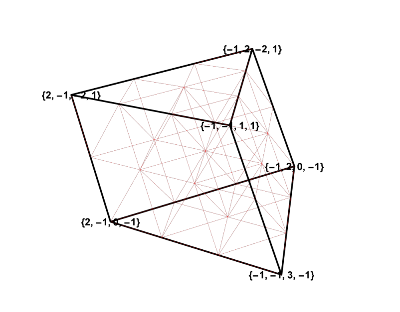
Figure 4. Tessellation of the plane arising from arranging the blades ((,,,,,))((1,2,3)) and ((,,,,,))((1,3,2)) on the root lattice of S​L3SL_{3}. See [50], as well as [45], where such structures have appeared in the context of representation theory.

It is interesting that Richard Feynman came rather near to the definition of blade arrangements more than 70 years ago, in his diagrammatic representation of perturbative Quantum Field Theory. However, the key structures in combinatorial geometry had yet not been been developed formally.

It turns out that (tree-level) Feynman Diagrams are dual to blade arrangements on the hypersimplex Δ2,n\Delta_{2,n}, not only combinatorially but realizably, in the sense of tropical geometry: in general, start with a subdivision of a polytope into a number of maximal cells. Then place a vertex in the middle of each cell and connect with an edge any pair of vertices that is separated by an internal facet. For certain polytopes and certain finest matroid subdivisions of them, the result of this process is a tree, and in the case that the polytope is the hypersimplex Δ2,n\Delta_{2,n}, then varying over all such finest regular subdivisions one obtains all (2​n−5)!!(2n-5)!! Feynman diagrams occurring in the cubic scalar at tree-level, and in particular all Cn−2C_{n-2} planar tree-level Feynman diagrams in the biadjoint scalar amplitude have a prominent role, where Cn−2=2,5,14,…C_{n-2}=2,5,14,\ldots, is the Catalan number: such trees are in bijection with a restricted set of subdivisions that are regular and positroidal when the cyclic order is the standard one, α=(12⋯n)\alpha=(12\cdots n).

Feynman diagrams have a natural higher dimensional holographic-type generalization on faces of the hypersimplex. Borges-Cachazo [9] discovered the prototype for Feynman diagrams for generalized scattering amplitudes, consisting of compatible collections of Feynman diagrams on the nn facets of the hypersimplex Δ3,n\Delta_{3,n}. This was developed further in [22, 30, 35]. See also [36].

However this is only part of the picture: this description amounts to a holographic representation of a dual blade arrangement which is defined in the interior of the hypersimplex Δk,n\Delta_{k,n}; but it is not a priori clear all of the information from the interior of the hypersimplex should be preserved in the process of passing to such a high codimension boundary, particularly for large kk and nn. Moreover, in the generalized Feynman diagram model there is no preferred notion of a standard basis for the dual kinematic space. However, blade arrangements not only resolve this ambiguity, but they do so canonically, in the sense that there is one such basis for each cyclic order. Therefore, in the blade model planarity is emergent. A priori, for the generalized biadjoint scalar there is no systematic method to check when two singularities are compatible; also, there are just too many of them! One has to run a complicated algorithm on the computer every time which becomes infeasible quickly beyond the simplest cases; this suggests again that there is more to the story and it begs for a simpler and more straightforward model to study first. Indeed, searching for a scattering amplitude whose possible singularities are limited to the (nk)−n\binom{n}{k}-n blades on the hypersimplex Δk,n\Delta_{k,n}, then one is pulled inexorably to the construction in this paper of an amplitude and worldsheet which are so simple, belying the very rich combinatorial structures that they encode, that hand computations are again possible: one can check with a pencil and paper whether two poles are compatible, using a simple noncrossing rule on kk-tuples of integers which specializes to the Steinmann compatibility relations for poles of the cubic scalar amplitude when k=2k=2, and which is distinct from – and in some respects much better behaved than – the closely related combinatorial notion of weak separation. The geometric content of the noncrossing rule is that the generalized root polytope ℛn−k(k)\mathcal{R}^{(k)}_{n-k}, introduced in [24], should be given a very particular flag unimodular triangulation with Cn−k(k)C^{(k)}_{n-k} maximal simplices, where Cn−k(k)C^{(k)}_{n-k} is a richly structured integer in combinatorics, the kk-dimensional Catalan number, O.E.I.S. number A060854 [46].

Let us conclude the introduction with a blade-theoretic calculation of the biadjoint scalar m(2)​(𝕀6,𝕀6)m^{(2)}(\mathbb{I}_{6},\mathbb{I}_{6}) (see [16] for the Definition) at a manifestly planar kinematic point. Explicitly, we specify values for the basis of the kinematic space which is emergent from the blade model; otherwise in this paper we are concerned with the analogous situation for all generalized amplitudes with k≥2k\geq 2.

Later on, we will interpret the variables αj\alpha_{j} as simple roots and then add a second index, αi,j\alpha_{i,j} where i=1,…,k−1i=1,\ldots,k-1 and j=1,…,n−kj=1,\ldots,n-k. Many of the enumerative results for the k=2k=2 root lattice carries over to k≥3k\geq 3, including for instance the triangulation of the root polytope, the convex hull of the positive roots and the origin, into simplices which are in bijection with certain alternating trees, see [34, 50, 43].
Refer to caption
Figure 5. Example 1.11: associahedron for the degenerate (2,6)(2,6) biadjoint scalar amplitude m(2)​(𝕀6,𝕀6)m^{(2)}(\mathbb{I}_{6},\mathbb{I}_{6}) corresponding to the kinematics in Equation (1.11). Feynman diagrams are identified with labeled (boundary) vertices. Red lines are added to indicate compatibility with the root lattice, with directions ei−eje_{i}-e_{j}. Also the Newton polytope for argument of the log in the potential function at the point (α)=(0,0,0,0)(\alpha)=(0,0,0,0) in Equation (1.11), ( x 1,1 +x 1,2 +x 1,3 ) 3 ( x 1,3 +x 1,4 ) 2 x 1,1 x 1,2 x 1,3 2 x 1,4 .
Example 1.11.

Consider the kinematic point (s)(s) specified1010 10 Here we are not giving directly the values of the si​js_{ij}’s, but they are easy to derive, by solving the 99 equations here, together with 6 equations ηi​i+1=0\eta_{i\ i+1}=0, which are automatically satisfied on the kinematic (sub)space 𝒦2,n\mathcal{K}_{2,n} of ℝ(n2)\mathbb{R}^{\binom{n}{2}}. by the values of the planar kinematic invariants ηi​j\eta_{ij},

η13η14η15η24η25η26η35η36η46α1+1α12+2α123+1α2+1α23+3α234+2α3+2α34+1α4+1\displaystyle\begin{array}[]{ccccccccc}\eta_{13}&\eta_{14}&\eta_{15}&\eta_{24}&\eta_{25}&\eta_{26}&\eta_{35}&\eta_{36}&\eta_{46}\\ \alpha_{1}+1&\alpha_{12}+2&\alpha_{123}+1&\alpha_{2}+1&\alpha_{23}+3&\alpha_{234}+2&\alpha_{3}+2&\alpha_{34}+1&\alpha_{4}+1\end{array}

where we denote αJ=∑j∈Jαj\alpha_{J}=\sum_{j\in J}\alpha_{j} for a subset JJ of {1,2,3,4}\{1,2,3,4\}, so for instance α23=α2+α3\alpha_{23}=\alpha_{2}+\alpha_{3}. Here αj\alpha_{j} are coordinate functions on ℝ4\mathbb{R}^{4}.

For the resulting potential function

𝒮2,6=log⁡(x1,1α1​x1,2α2​x1,3α3​x1,4α4(x1,1+x1,2+x1,3+x1,4)α1234)+log⁡(x1,1​x1,2​x1,32​x1,4(x1,1+x1,2+x1,3)3​(x1,3+x1,4)2),\mathcal{S}_{2,6}=\log\left(\frac{x_{1,1}^{\alpha_{1}}x_{1,2}^{\alpha_{2}}x_{1,3}^{\alpha_{3}}x_{1,4}^{\alpha_{4}}}{(x_{1,1}+x_{1,2}+x_{1,3}+x_{1,4})^{\alpha_{1234}}}\right)+\log\left(\frac{x_{1,1}x_{1,2}x_{1,3}^{2}x_{1,4}}{\left(x_{1,1}+x_{1,2}+x_{1,3}\right)^{3}\left(x_{1,3}+x_{1,4}\right)^{2}}\right),

applying for instance the CHY scattering equations formalism can be shown to give, when α1+α2+α3+α4=0\alpha_{1}+\alpha_{2}+\alpha_{3}+\alpha_{4}=0, for the biadjoint scalar amplitude1111 11 Abbreviating m6(2)=m(2)​(𝕀6,𝕀6)m^{(2)}_{6}=m^{(2)}(\mathbb{I}_{6},\mathbb{I}_{6}), where we abbreviate 𝕀6=(123456)\mathbb{I}_{6}=(123456). For our purposes, this equation may be taken as a definition.

(17) m6(2)\displaystyle m^{(2)}_{6} =\displaystyle= 1η14​η15​η24+1η15​η24​η25+1η24​η25​η26+1η13​η15​η35+1η15​η25​η35+1η25​η26​η35\displaystyle\frac{1}{\eta_{14}\eta_{15}\eta_{24}}+\frac{1}{\eta_{15}\eta_{24}\eta_{25}}+\frac{1}{\eta_{24}\eta_{25}\eta_{26}}+\frac{1}{\eta_{13}\eta_{15}\eta_{35}}+\frac{1}{\eta_{15}\eta_{25}\eta_{35}}+\frac{1}{\eta_{25}\eta_{26}\eta_{35}}
+\displaystyle+ 1η13​η14​η15+1η26​η35​η36+1η13​η14​η46+1η14​η24​η46+1η24​η26​η46+1η13​η36​η46\displaystyle\frac{1}{\eta_{13}\eta_{14}\eta_{15}}+\frac{1}{\eta_{26}\eta_{35}\eta_{36}}+\frac{1}{\eta_{13}\eta_{14}\eta_{46}}+\frac{1}{\eta_{14}\eta_{24}\eta_{46}}+\frac{1}{\eta_{24}\eta_{26}\eta_{46}}+\frac{1}{\eta_{13}\eta_{36}\eta_{46}}
+\displaystyle+ 1η26​η36​η46+1η13​η35​η36,\displaystyle\frac{1}{\eta_{26}\eta_{36}\eta_{46}}+\frac{1}{\eta_{13}\eta_{35}\eta_{36}},

the following reduced Feynman diagram expansion around maximal collections of compatible poles,

(18) m6(2)\displaystyle m^{(2)}_{6} =\displaystyle= 1(α1+1)​(α4+1)​(α34+1)+1(α2+1)​(α4+1)​(α34+1)+1(α1+1)​(α2+1)​(α4+1)\displaystyle\frac{1}{\left(\alpha_{1}+1\right)\left(\alpha_{4}+1\right)\left(\alpha_{34}+1\right)}+\frac{1}{\left(\alpha_{2}+1\right)\left(\alpha_{4}+1\right)\left(\alpha_{34}+1\right)}+\frac{1}{\left(\alpha_{1}+1\right)\left(\alpha_{2}+1\right)\left(\alpha_{4}+1\right)}
+\displaystyle+ 1(α1+1)​(α34+1)​(α123+1)+1(α2+1)​(α34+1)​(α123+1)\displaystyle\frac{1}{\left(\alpha_{1}+1\right)\left(\alpha_{34}+1\right)\left(\alpha_{123}+1\right)}+\frac{1}{\left(\alpha_{2}+1\right)\left(\alpha_{34}+1\right)\left(\alpha_{123}+1\right)}
+\displaystyle+ 1(α1+1)​(α2+1)​(α123+1).\displaystyle\frac{1}{\left(\alpha_{1}+1\right)\left(\alpha_{2}+1\right)\left(\alpha_{123}+1\right)}.

See Figure 5 for the polytope cut out in the α\alpha-space by the requirement that all poles ηi​j\eta_{ij} must be nonnegative. Then the six terms correspond directly to the six vertices of the polytope; the function itself is positive on the interior of the polytope, with poles on the facets.

In the next section, we state and prove our results for the lattice of points in a subspace ℋk,n\mathcal{H}_{k,n} (see Equation (4)) rather than the lattice of linear functions in the dual space, keeping in mind that the two are naturally (if not canonically) isomorphic.

2. Kinematic Space and Planar Basis

Fix integers (k,n)(k,n) such that 1≤k≤n−11\leq k\leq n-1.

Recall the notation ([n]k)\binom{[n]}{k} for the set of kk-element subsets of the set [n]={1,…,n}[n]=\{1,\ldots,n\}, and denote by

([n]k)n​f=([n]k)∖{{j,j+1,…,j+k−1}:j=1,…,n}\binom{[n]}{k}^{nf}=\binom{[n]}{k}\setminus\left\{\{j,j+1,\ldots,j+k-1\}:j=1,\ldots,n\right\}

the nonfrozen kk-element subsets. Let {eJ:J∈([n]k)}\{e^{J}:J\in\binom{[n]}{k}\} be the standard basis for ℝ(nk)\mathbb{R}^{\binom{n}{k}}.

The kthk^{\text{th}} hypersimplex in nn variables is the kthk^{\text{th}} integer cross-section of the unit cube [0,1]n[0,1]^{n},

Δk,n={x∈[0,1]n:∑xj=k}.\Delta_{k,n}=\left\{x\in[0,1]^{n}:\sum x_{j}=k\right\}.

Henceforth we shall assume that 2≤k≤n−22\leq k\leq n-2.

Recall that the lineality space is the n-dimensional subspace

{∑JxJ​eJ:x∈ℝn},\left\{\sum_{J}x_{J}e^{J}:x\in\mathbb{R}^{n}\right\},

of ℝ(nk)\mathbb{R}^{\binom{n}{k}}, where we use the notation xJ=∑j∈Jxjx_{J}=\sum_{j\in J}x_{j}.

Then the kinematic space is the dimension (nk)−n\binom{n}{k}-n subspace of ℝ(nk)\mathbb{R}^{\binom{n}{k}},

(19) 𝒦(k,n)={(s)∈ℝ(nk):∑J:J∋jsJ=0,j=1,…,n}.\displaystyle\mathcal{K}(k,n)=\left\{(s)\in\mathbb{R}^{\binom{n}{k}}:\sum_{J:\ J\ni j}s_{J}=0,\ j=1,\ldots,n\right\}.

Now for any J∈([n]k)n​fJ\in\binom{[n]}{k}^{nf}, define a linear functional on the kinematic space, or in more physical terminology, a planar kinematic invariant, ηJ:𝒦⁡(k,n)→ℝ\eta_{J}:\mathcal{K}(k,n)\rightarrow\mathbb{R}, by

(20) ηJ​(s)\displaystyle\eta_{J}(s) =\displaystyle= −1n∑I∈([n]k)min{L1(eI−eJ),…,Ln(eI−eJ)}sI,\displaystyle-\frac{1}{n}\sum_{I\in\binom{[n]}{k}}\min\{L_{1}(e_{I}-e_{J}),\ldots,L_{n}(e_{I}-e_{J})\}s_{I},

where

Lj​(x)=xj+1+2​xj+2+⋯+(n−1)​xj−1L_{j}(x)=x_{j+1}+2x_{j+2}+\cdots+(n-1)x_{j-1}

for j=1,…,nj=1,\ldots,n are linear functions on ℝn\mathbb{R}^{n}.

Usually instead of ηJ​(s)\eta_{J}(s) we write just ηJ\eta_{J} with the understanding that ηJ\eta_{J} is to be evaluated on points (s)∈𝒦⁡(k,n)(s)\in\mathcal{K}(k,n).

Then we have the property that if J={i,i+1,…,i+k−1}J=\{i,i+1,\ldots,i+k-1\} is frozen, then since the graph of ρJ:Δk,n→ℝ\rho_{J}:\Delta_{k,n}\rightarrow\mathbb{R} does not bend over Δk,n\Delta_{k,n}, it follows that ηJ\eta_{J} is identically zero on 𝒦⁡(k,n)\mathcal{K}(k,n). See [31] for details.

A further computation proves linear independence for the set of ηJ\eta_{J} where JJ is nonfrozen, and we obtain Proposition 2.1.

Proposition 2.1 ([30, 31]).

The set of linear functions

{ηJ:𝒦(k,n)→ℝ:J∈([n]k)n​f}\left\{\eta_{J}:\mathcal{K}(k,n)\rightarrow\mathbb{R}:J\in\binom{[n]}{k}^{nf}\right\}

is a basis of the space of the dual kinematic space (𝒦⁡(k,n))∗\left(\mathcal{K}(k,n)\right)^{\ast}, that is to say, it is a basis of the space of linear functions on 𝒦⁡(k,n)\mathcal{K}(k,n).

3. Root Polytopes and Triangulations

In this section, we introduce the generalized root polytope ℛn−k(k)\mathcal{R}^{(k)}_{n-k}, which is most conveniently defined in the space of linear functions on ℋk,n\mathcal{H}_{k,n}.

Put αi,[a,b]=∑j=abαi,j\alpha_{i,[a,b]}=\sum_{j=a}^{b}\alpha_{i,j}. Let J={j1,…,jk}J=\{j_{1},\ldots,j_{k}\}, with order 1≤j1<⋯<jk≤n1\leq j_{1}<\cdots<j_{k}\leq n. The generalized positive root γJ\gamma_{J} is the following sum of simple roots αi,j\alpha_{i,j}:

γJ​(α)=∑i=1k−1αi,[ji−(i−1),ji+1−i−1].\gamma_{J}(\alpha)=\sum_{i=1}^{k-1}\alpha_{i,[j_{i}-(i-1),j_{i+1}-i-1]}.
Figure 6. A generalized positive root.
Definition 3.1.

The root polytope ℛn−k(k)\mathcal{R}^{(k)}_{n-k} is the convex hull

ℛn−k(k)=convex hull({γJ:ℋk,n→ℝ:J∈([n]k)n​f}).\mathcal{R}^{(k)}_{n-k}=\text{convex hull}\left(\left\{\gamma_{J}:\mathcal{H}_{k,n}\rightarrow\mathbb{R}:J\in\binom{[n]}{k}^{nf}\right\}\right).

We also denote by ℛ^n−k(k)\hat{\mathcal{R}}^{(k)}_{n-k} the convex hull

ℛ^n−k(k)=convex hull({0},{γJ:ℝ(k−1)×(n−k)→ℝ:J∈([n]k)n​f}).\hat{\mathcal{R}}^{(k)}_{n-k}=\text{convex hull}\left(\{0\},\left\{\gamma_{J}:\mathbb{R}^{(k-1)\times(n-k)}\rightarrow\mathbb{R}:J\in\binom{[n]}{k}^{nf}\right\}\right).

Here the polytope ℛn−k(k)\mathcal{R}^{(k)}_{n-k} has dimension (k−1)​(n−k−1)(k-1)(n-k-1), while the polytope ℛ^n−k(k)\hat{\mathcal{R}}^{(k)}_{n-k} has dimension (k−1)​(n−k)(k-1)(n-k). These polytopes may be of independent interest; however, in what follows we concentrate on the smaller-dimensional polytope ℛn−k(k)\mathcal{R}^{(k)}_{n-k}.

We may decide to embed ℛn−k(k)\mathcal{R}^{(k)}_{n-k} into ℋk,n\mathcal{H}_{k,n} by identifying the space of linear functions on ℋk,n\mathcal{H}_{k,n} with ℋk,n\mathcal{H}_{k,n} itself, with respect to the dual pairing αi,j​(ei′,j′)=δi,i′​δj,j′\alpha_{i,j}(e_{i^{\prime},j^{\prime}})=\delta_{i,i^{\prime}}\delta_{j,j^{\prime}}; then we may take ℛn−k(k)\mathcal{R}^{(k)}_{n-k} to be the projection of the polytope ℛ^n−k(k)\hat{\mathcal{R}}^{(k)}_{n-k}. To connect with the type AA root polytope, see [34, 50, 43], the convex hull of the positive roots ei−eje_{i}-e_{j} for 1≤i<j≤n1\leq i<j\leq n, together with the origin, define a projection pk,n:ℝ(k−1)×(n−k)→ℋk,np_{k,n}:\mathbb{R}^{(k-1)\times(n-k)}\rightarrow\mathcal{H}_{k,n} by pk,n​(ei,j)=fi,jp_{k,n}(e_{i,j})=f_{i,j}, where

fi,j={ei,j−ei,j+1, 1≤j≤n−k−1ei,n−k−ei,1,j=n−k.f_{i,j}=\begin{cases}e_{i,j}-e_{i,j+1},&\ 1\leq j\leq n-k-1\\ e_{i,n-k}-e_{i,1},&\ j=n-k.\end{cases}

Now for each J∈([n]k)J\in\binom{[n]}{k}, define

(21) v^J\displaystyle\hat{v}_{J} =\displaystyle= ∑ℓ=1k−1eℓ,[jℓ−(ℓ−1),jℓ+1−ℓ−1]\displaystyle\sum_{\ell=1}^{k-1}e_{\ell,[j_{\ell}-(\ell-1),j_{\ell+1}-\ell-1]}
vJ\displaystyle v_{J} =\displaystyle= ∑ℓ=1k−1fℓ,[jℓ−(ℓ−1),jℓ+1−ℓ−1]\displaystyle\sum_{\ell=1}^{k-1}f_{\ell,[j_{\ell}-(\ell-1),j_{\ell+1}-\ell-1]}

Evidently vJv_{J} is zero exactly when JJ is a single cyclic interval, and v^J\hat{v}_{J} is zero exactly when JJ has is an interval of the form [i,i+k−1][i,i+k-1] for 1≤i1\leq i and i+k−1≤ni+k-1\leq n.

Generalized roots satisfy certain cubical relations, of which the usual square move, or flip move, is a special case. We formulate them on the hypersimplex Δk,n\Delta_{k,n}.

For any integers 2≤m≤k2\leq m\leq k, then any intersection of affine hyperplanes in ℝn\mathbb{R}^{n}, say

xi1+xj1=xi2+xj2=⋯=xim+xjm=1,x_{i_{1}}+x_{j_{1}}=x_{i_{2}}+x_{j_{2}}=\cdots=x_{i_{m}}+x_{j_{m}}=1,

intersects the hypersimplex Δk,n\Delta_{k,n}; we specialize to the case when 1≤i1<j1<i2<j2<⋯<im<jm≤n1\leq i_{1}<j_{1}<i_{2}<j_{2}<\cdots<i_{m}<j_{m}\leq n. Taking any subset L={ℓ1,…,ℓk−m}∈([n]∖(I∪J)k−m)L=\{\ell_{1},\ldots,\ell_{k-m}\}\in\binom{[n]\setminus(I\cup J)}{k-m}, then we define an mm-dimensional cube in Δk,n\Delta_{k,n},

𝒞I,J(L)={x∈Δk,n:xia+xja=1 and xℓb=1 for a=1,…,m;b=1,…,k−m}.\mathcal{C}^{(L)}_{I,J}=\left\{x\in\Delta_{k,n}:x_{i_{a}}+x_{j_{a}}=1\text{ and }\ x_{\ell_{b}}=1\text{ for }a=1,\ldots,m;\ b=1,\ldots,k-m\right\}.
Proposition 3.2.

Given any pair of long diagonals of 𝒞I,J(L)\mathcal{C}^{(L)}_{I,J} specified by the pairs of vertices of Δk,n\Delta_{k,n}, respectively (eM1∪L,eM2∪L)(e_{M_{1}\cup L},\ e_{M_{2}\cup L}) and (eM1′∪L,eM2′∪L)(e_{M^{\prime}_{1}\cup L},\ e_{M^{\prime}_{2}\cup L}), then we have that

(22) vM1∪L+vM2∪L\displaystyle v_{M_{1}\cup L}+v_{M_{2}\cup L} =\displaystyle= vM1′∪L+vM2′∪L\displaystyle v_{M^{\prime}_{1}\cup L}+v_{M^{\prime}_{2}\cup L}

and correspondingly

γM1∪L+γM2∪L\displaystyle\gamma_{M_{1}\cup L}+\gamma_{M_{2}\cup L} =\displaystyle= γM1′∪L+γM2′∪L.\displaystyle\gamma_{M^{\prime}_{1}\cup L}+\gamma_{M^{\prime}_{2}\cup L}.

Moreover, for each such cubical cell, there exists a unique pair of antipodal vertices of 𝒞I,J(L)\mathcal{C}^{(L)}_{I,J} that is noncrossing, namely (eM1′′∪L,eM2′′∪L)(e_{M^{\prime\prime}_{1}\cup L},e_{M^{\prime\prime}_{2}\cup L}), where

M1′′\displaystyle M^{\prime\prime}_{1} =\displaystyle= {i1,j2,i3,j4,…,im−1,jm}\displaystyle\{i_{1},j_{2},i_{3},j_{4},\ldots,i_{m-1},j_{m}\}
M2′′\displaystyle M^{\prime\prime}_{2} =\displaystyle= {j1,i2,j3,i4,…,jm−1,im}.\displaystyle\{j_{1},i_{2},j_{3},i_{4},\ldots,j_{m-1},i_{m}\}.

For instance, recalling that γ145+γ236=α1,12+α2,23\gamma_{145}+\gamma_{236}=\alpha_{1,12}+\alpha_{2,23}, it follows easily that

γ145+γ236=γ245+γ136=γ135+γ246=γ146+γ235.\gamma_{145}+\gamma_{236}=\gamma_{245}+\gamma_{136}=\gamma_{135}+\gamma_{246}=\gamma_{146}+\gamma_{235}.

Here {145,236}\{145,236\} is the only noncrossing (but not weakly separated) pair among these.

For instance, letting I={1,3,5,7,9,11}I=\{1,3,5,7,9,11\} and J={2,4,6,8,10,12}J=\{2,4,6,8,10,12\}, then the pair

({1,4,5,8,9,12},{2,3,6,7,10,11})(\{1,4,5,8,9,12\},\{2,3,6,7,10,11\})

for n≥12n\geq 12, is noncrossing and we have the corresponding four-term identity:

v1,3,5,7,9,11+v2,4,6,8,10,12=v1,4,5,8,9,12+v2,3,6,7,10,11.v_{1,3,5,7,9,11}+v_{2,4,6,8,10,12}=v_{1,4,5,8,9,12}+v_{2,3,6,7,10,11}.

Let us conclude with two instructive examples. With L={6,10}L=\{6,10\}, then

γ1,3,5,6,10+γ2,4,6,8,10=γ1,4,5,6,10+γ2,3,6,8,10.\gamma_{1,3,5,6,10}+\gamma_{2,4,6,8,10}=\gamma_{1,4,5,6,10}+\gamma_{2,3,6,8,10}.

where the pair {{1,4,5,6,10},{2,3,6,8,10}}\{\{1,4,5,6,10\},\{2,3,6,8,10\}\} is noncrossing. This shows, in particular, that the set LL can be interlaced with the indices defining the cube CI,J(L)C^{(L)}_{I,J}. This works from a combinatorial point of view due to the requirement that weak separation can be violated when the respective interior intervals are not the same, but what if we didn’t know this rule and had only the formal definition of the linear functions γJ\gamma_{J}? The explicit identities are:

(23) γ1,3,5,6,10+γ2,4,6,8,10\displaystyle\gamma_{1,3,5,6,10}+\gamma_{2,4,6,8,10} =\displaystyle= (α1,1+α2,2+α4,3)+(α1,2+α2,3+α3,4)\displaystyle(\alpha_{1,1}+\alpha_{2,2}+\alpha_{4,3})+(\alpha_{1,2}+\alpha_{2,3}+\alpha_{3,4})
(24) γ1,4,5,6,10+γ2,3,6,8,10\displaystyle\gamma_{1,4,5,6,10}+\gamma_{2,3,6,8,10} =\displaystyle= (α1,1+α1,2+α4,3)+(α2,2+α2,3+α3,4)\displaystyle(\alpha_{1,1}+\alpha_{1,2}+\alpha_{4,3})+(\alpha_{2,2}+\alpha_{2,3}+\alpha_{3,4})

Finally, letting I={1,3,5,7,9,11}I=\{1,3,5,7,9,11\} and J={2,4,6,8,10,12}J=\{2,4,6,8,10,12\}, then for the pair

({1,4,5,8,9,12},{2,3,6,7,10,11})∈𝐍𝐂6,12∖𝐖𝐒6,12(\{1,4,5,8,9,12\},\{2,3,6,7,10,11\})\in\mathbf{NC}_{6,12}\setminus\mathbf{WS}_{6,12}

we have the following four-term identity:

γ1,3,5,7,9,11+γ2,4,6,8,10,12=γ1,4,5,8,9,12+γ2,3,6,7,10,11.\gamma_{1,3,5,7,9,11}+\gamma_{2,4,6,8,10,12}=\gamma_{1,4,5,8,9,12}+\gamma_{2,3,6,7,10,11}.

As a special case of the cubical relations, we recover the usual flip move.

Corollary 3.3.

The linear functions γJ\gamma_{J} (as well as the vectors vJv_{J}) satisfy the following additive relation: supposing that I∪{a,b,c,d}∈([n]k+2)I\cup\{a,b,c,d\}\in\binom{[n]}{k+2} with a<b<c<da<b<c<d, then we have

(25) γI​a​c+γI​b​d\displaystyle\gamma_{Iac}+\gamma_{Ibd} =\displaystyle= γI​a​d+γI​b​c.\displaystyle\gamma_{Iad}+\gamma_{Ibc}.

Given a<b<c<da<b<c<d such that {b}∪I∪{c}∈([n]k)\{b\}\cup I\cup\{c\}\in\binom{[n]}{k} is a single subinterval of {1,2,…,n}\{1,2,\ldots,n\}, then as a specialization of Equation (25) we obtain Equation (26),

(26) γI​a​c+γI​b​d=γI​a​d.\displaystyle\gamma_{Iac}+\gamma_{Ibd}=\gamma_{Iad}.

When k=2k=2 (and I=∅I=\emptyset), then Equations (25) and (26) are equivalent (pulling back via the projection p2,np_{2,n}) to the following somewhat more familiar relations among roots, respectively

(α1,a−α1,c−1)+(α1,b−α1,d−1)=(α1,a−α1,d−1)+(α1,b−α1,c−1).(\alpha_{1,a}-\alpha_{1,c-1})+(\alpha_{1,b}-\alpha_{1,d-1})=(\alpha_{1,a}-\alpha_{1,d-1})+(\alpha_{1,b}-\alpha_{1,c-1}).

and

(α1,a−α1,c−1)+(α1,c−1−α1,d)=α1,a−α1,d.(\alpha_{1,a}-\alpha_{1,c-1})+(\alpha_{1,c-1}-\alpha_{1,d})=\alpha_{1,a}-\alpha_{1,d}.

4. Triangulation

Denote by ℒn−k(k)⊂ℋk,n\mathcal{L}^{(k)}_{n-k}\subset\mathcal{H}_{k,n} the (k−1)​(n−k−1)(k-1)(n-k-1)-dimensional integer lattice generated by the elements fi,j=pk,n​(ei,j)f_{i,j}=p_{k,n}(e_{i,j}), for (i,j)∈[1,k−1]×[1,n−k−1](i,j)\in[1,k-1]\times[1,n-k-1]. In particular, for our choice of projection pk,np_{k,n} then ℒn−k(k)\mathcal{L}^{(k)}_{n-k} is a Cartesian product of k−1k-1 root lattices of type S​Ln−kSL_{n-k}.

In what follows, we identify the k−1k-1 lattices as vj1​j2(i)=v[j1,j1+i−1]∪[j2+k−1−i,j2+k−2]v^{(i)}_{j_{1}j_{2}}=v_{[j_{1},j_{1}+i-1]\cup[j_{2}+k-1-i,j_{2}+k-2]}. For instance, with (k,n)=(4,9)(k,n)=(4,9), say, then

v36(1)=v3678=f1,3+f1,4,v36(2)=v3478=f2,3+f2,4,v36(3)=v3458=f3,3+f3,4.v^{(1)}_{36}=v_{3678}=f_{1,3}+f_{1,4},\ \ v^{(2)}_{36}=v_{3478}=f_{2,3}+f_{2,4},\ \ v^{(3)}_{36}=v_{3458}=f_{3,3}+f_{3,4}.

A key property of the elements fi,j∈ℋk,nf_{i,j}\in\mathcal{H}_{k,n} is that for each i=1,…,k−1i=1,\ldots,k-1, then fi,1,…,fi,n−kf_{i,1},\ldots,f_{i,n-k} span a subspace of dimension n−k−1n-k-1, satisfying the single relation

fi,1+⋯+fi,n−k=0.f_{i,1}+\cdots+f_{i,n-k}=0.
Lemma 4.1.

For each given i=1,…,k−1i=1,\ldots,k-1, then the embedding {j1,j2}↦[j1,j1+(i−1)]∪[j2,j2+(k−(i−1))]\{j_{1},j_{2}\}\mapsto[j_{1},j_{1}+(i-1)]\cup[j_{2},j_{2}+(k-(i-1))] has the following property: the pair {{j1,j2},{j3,j4}}\{\{j_{1},j_{2}\},\{j_{3},j_{4}\}\} is noncrossing (and thus is an edge in 𝐍𝐂2,n\mathbf{NC}_{2,n}) if and only if the image

{[j1,j1+(i−1)]∪[j2,j2+(k−(i−1))],[j3,j3+(i−1)]∪[j4,j4+(k−(i−1))]}\{[j_{1},j_{1}+(i-1)]\cup[j_{2},j_{2}+(k-(i-1))],[j_{3},j_{3}+(i-1)]\cup[j_{4},j_{4}+(k-(i-1))]\}

forms a noncrossing pair (and thus is an edge in 𝑂𝑃𝐸𝑁𝐍𝐂k,n+(k−2))\mathbf{NC}_{k,n+(k-2)}).

According to Proposition 4.2, given any maximal noncrossing collection

𝒥={J1,…,J(k−1)​(n−k−1)}∈𝐍𝐂k,n\mathcal{J}=\left\{J_{1},\ldots,J_{(k-1)(n-k-1)}\right\}\in\mathbf{NC}_{k,n}

then the cone ⟨𝒥⟩+\langle\mathcal{J}\rangle_{+}, defined by

⟨𝒥⟩+={∑j=1(k−1)​(n−k−1)tj​vJj:tj≥0},\langle\mathcal{J}\rangle_{+}=\left\{\sum_{j=1}^{(k-1)(n-k-1)}t_{j}v_{J_{j}}:t_{j}\geq 0\right\},

is simplicial and unimodular (so, the primitive integer generators of its rays, together with the origin, form the vertices of a simplex of volume 1/((k−1)​(n−k−1))!1/((k-1)(n-k-1))! where (k−1)​(n−k−1)(k-1)(n-k-1) is the dimension of the ambient space).

Proposition 4.2.

Given any maximal non-crossing collection 𝒥={J1,…,J(k−1)​(n−k−1)}∈𝐍𝐂k,n\mathcal{J}=\left\{J_{1},\ldots,J_{(k-1)(n-k-1)}\right\}\in\mathbf{NC}_{k,n} of nonfrozen subsets Ji∈([n]k)n​fJ_{i}\in\binom{[n]}{k}^{nf}, then the polyhedral cone ⟨𝒥⟩+\langle\mathcal{J}\rangle_{+} is simplicial of dimension (k−1)​(n−k−1)(k-1)(n-k-1). Moreover, any pair of simplices of the form

Convex hull​({0}∪{vJ:J∈𝒥1}),Convex hull​({0}∪{vJ:J∈𝒥2})\text{Convex hull}\left(\{0\}\cup\left\{v_{J}:J\in\mathcal{J}_{1}\right\}\right),\ \text{Convex hull}\left(\{0\}\cup\left\{v_{J}:J\in\mathcal{J}_{2}\right\}\right)

for 𝒥1,𝒥2∈𝐍𝐂k,n\mathcal{J}_{1},\mathcal{J}_{2}\in\mathbf{NC}_{k,n} maximal noncrossing collections, are related by a unique volume-preserving integer linear transformation.

Proof.

We shall argue by induction on kk.

For the base step: both statements for ℛn−2(2)\mathcal{R}^{(2)}_{n-2} (with n≥4n\geq 4) translate directly to standard properties for the non-crossing triangulation [34, 50] of the type An−2A_{n-2} root polytope into simplices which are put in bijection with certain alternating trees. See also [43] and the references therein. The identification with positive roots is as follows: for any 1≤i<j≤n−11\leq i<j\leq n-1 we have ei−ej=vi,j+1e_{i}-e_{j}=v_{i,j+1}.

Now let 𝒥={J1,…,J(k−1)​(n−k−1)}∈𝐍𝐂k,n\mathcal{J}=\left\{J_{1},\ldots,J_{(k-1)(n-k-1)}\right\}\in\mathbf{NC}_{k,n} be any maximal non-crossing collection.

We will show that the set {vJ:J∈𝒥}\left\{v_{J}:J\in\mathcal{J}\right\} is a lattice basis, that is, any element in the ambient lattice ℒn−k(k)\mathcal{L}^{(k)}_{n-k} is a linear combination of the given vertices vJ∈ℛn−k(k)v_{J}\in\mathcal{R}^{(k)}_{n-k} for J∈𝒥J\in\mathcal{J} with integer coefficients. Indeed, in this case, any pair of maximal simplices labeled by maximal non-crossing collections are related by a volume-preserving (integer-valued) linear transformation.

We induct on kk using a partition of unity φk−2+φ−1=𝐢𝐝\varphi_{k-2}+\varphi_{-1}=\mathbf{id}.

Let φk−2:ℋk,n→ℋk−1,n\varphi_{k-2}:\mathcal{H}_{k,n}\rightarrow\mathcal{H}_{k-1,n} be the projection onto the first k−2k-2 rows, defined by φk−2:ei,j↦ei,j\varphi_{k-2}:e_{i,j}\mapsto e_{i,j} for 1≤i≤k−21\leq i\leq k-2 and ek−1,j↦0e_{k-1,j}\mapsto 0, for all j=1,…,(n−k)j=1,\ldots,(n-k). Define a second projection φ−1:ℋk,n(0)→ℋ2,n(0)\varphi_{-1}:\mathcal{H}^{(0)}_{k,n}\rightarrow\mathcal{H}^{(0)}_{2,n} onto the last row, by φ−1:ei,j↦0\varphi_{-1}:e_{i,j}\mapsto 0 for 1≤i≤k−21\leq i\leq k-2 and ek−1,j↦ek−1,je_{k-1,j}\mapsto e_{k-1,j}, for all j=1,…,(k−1)​(n−k)j=1,\ldots,(k-1)(n-k). Define

𝒥k−2={J∈𝒥:φk−2​(vJ)≠0}​ and ​𝒥−1={J∈𝒥:φ−1​(vJ)≠0}.\mathcal{J}_{k-2}=\left\{J\in\mathcal{J}:\varphi_{k-2}(v_{J})\not=0\right\}\text{ and }\mathcal{J}_{-1}=\left\{J\in\mathcal{J}:\varphi_{-1}(v_{J})\not=0\right\}.

Let v∈ℒn−k(k)v\in\mathcal{L}^{(k)}_{n-k} be an arbitrary lattice point. We claim that there exists a unique set of integers

{cJ∈ℤ:J∈𝒥}\{c_{J}\in\mathbb{Z}:J\in\mathcal{J}\}

such that

v=∑J∈𝒥cJ​vJ.v=\sum_{J\in\mathcal{J}}c_{J}v_{J}.

Now 𝒥k−2\mathcal{J}_{k-2} is a collection of kk-element subsets J={j1,…,jk}J=\{j_{1},\ldots,j_{k}\} wherein the largest two indices satisfy jk−1+1=jkj_{k-1}+1=j_{k}. Similarly, (𝒥−1∖𝒥k−2)(\mathcal{J}_{-1}\setminus\mathcal{J}_{k-2}) is a collection of kk-element subsets of the form J=[a,b]∪{j}J=[a,b]\cup\{j\} wherein only the largest two indices bb and jj are not adjacent.

Then, inducting on kk, it follows that the (noncrossing) collections 𝒥k−2\mathcal{J}_{k-2} and respectively (𝒥−1∖𝒥k−2)(\mathcal{J}_{-1}\setminus\mathcal{J}_{k-2}), the sets

{vJ:J∈𝒥k−2},{vJ:J∈(𝒥−1∖𝒥k−2)},\{v_{J}:J\in\mathcal{J}_{k-2}\},\ \ \{v_{J}:J\in(\mathcal{J}_{-1}\setminus\mathcal{J}_{k-2})\},

are lattice bases for their respective sublattices,

ℤ⁡{vJ:J∈𝒥k−2}≃ℒn−k(k−1)​ and ​ℤ​{vJ:J∈(𝒥−1∖𝒥k−2)}≃ℒn−k(2).\mathbb{Z}\left\{v_{J}:J\in\mathcal{J}_{k-2}\right\}\simeq\mathcal{L}^{(k-1)}_{n-k}\text{ and }\mathbb{Z}\left\{v_{J}:J\in(\mathcal{J}_{-1}\setminus\mathcal{J}_{k-2})\right\}\simeq\mathcal{L}^{(2)}_{n-k}.

Consequently there exist unique integers aJ,bJa_{J},b_{J} such that

φk−2​(v)=∑J∈𝒥k−2aJ​vJ,φ−1​(w)=∑J∈𝒥−1∖𝒥k−2bJ​vJ,\varphi_{k-2}(v)=\sum_{J\in\mathcal{J}_{k-2}}a_{J}v_{J},\ \ \varphi_{-1}(w)=\sum_{J\in\mathcal{J}_{-1}\setminus\mathcal{J}_{k-2}}b_{J}v_{J},

hence

(27) v\displaystyle v =\displaystyle= φk−2​(w)+φ−1​(w)\displaystyle\varphi_{k-2}(w)+\varphi_{-1}(w)
=\displaystyle= ∑J∈𝒥k−2aJ​vJ+∑J∈𝒥−1∖𝒥k−2bJ​vJ,\displaystyle\sum_{J\in\mathcal{J}_{k-2}}a_{J}v_{J}+\sum_{J\in\mathcal{J}_{-1}\setminus\mathcal{J}_{k-2}}b_{J}v_{J},
(28) =\displaystyle= ∑J∈𝒥cJ​vJ,\displaystyle\sum_{J\in\mathcal{J}}c_{J}v_{J},

where cJ=aJc_{J}=a_{J} if J∈𝒥k−2J\in\mathcal{J}_{k-2} and cJ=bJc_{J}=b_{J} if J∈𝒥−1∖𝒥k−2J\in\mathcal{J}_{-1}\setminus\mathcal{J}_{k-2}. ∎

Theorem 4.3.

Given any v∈ℋk,nv\in\mathcal{H}_{k,n}, then there exists a unique noncrossing collection 𝒥∈𝐍𝐂k,n\mathcal{J}\in\mathbf{NC}_{k,n} such that vv is in the relative interior of ⟨𝒥⟩+\langle\mathcal{J}\rangle_{+}. In particular, the set of cones

{⟨𝒥⟩+:𝒥∈𝐍𝐂k,n}\left\{\langle\mathcal{J}\rangle_{+}:\mathcal{J}\in\mathbf{NC}_{k,n}\right\}

defines a complete simplicial fan.

Proof.

We show that any point in ℋk,n\mathcal{H}_{k,n} lies in the relative interior of a unique simplicial cone ⟨𝒥⟩+\langle\mathcal{J}\rangle_{+} where 𝒥∈𝐍𝐂k,n\mathcal{J}\in\mathbf{NC}_{k,n} is a noncrossing collection.

We induct on kk, using the partition of unity φk−2+φ−1=𝐢𝐝\varphi_{k-2}+\varphi_{-1}=\mathbf{id} to prepare the induction step as in the proof of Proposition 4.2. Let us repeat the construction for sake of proximity.

Denote by φk−2:ℋk,n→ℋk,n\varphi_{k-2}:\mathcal{H}_{k,n}\rightarrow\mathcal{H}_{k,n} the projection φk−2:ei,j↦ei,j\varphi_{k-2}:e_{i,j}\mapsto e_{i,j} for 1≤i≤k−21\leq i\leq k-2 and ek−1,j↦0e_{k-1,j}\mapsto 0, for all j=1,…,(n−k)j=1,\ldots,(n-k). Define a second projection φ−1:ℋk,n→ℋk,n\varphi_{-1}:\mathcal{H}_{k,n}\rightarrow\mathcal{H}_{k,n} by φ−1:ei,j↦0\varphi_{-1}:e_{i,j}\mapsto 0 for 1≤i≤k−21\leq i\leq k-2 and ek−1,j↦ek−1,je_{k-1,j}\mapsto e_{k-1,j}, for all j=1,…,(n−k)j=1,\ldots,(n-k). Evidently we have φk−2​(ℋk,n)≃ℋk−1,n−1\varphi_{k-2}(\mathcal{H}_{k,n})\simeq\mathcal{H}_{k-1,n-1} and φ−1​(ℋk,n)≃ℋ2,n−(k−2)\varphi_{-1}(\mathcal{H}_{k,n})\simeq\mathcal{H}_{2,n-(k-2)}. Finally, again set

𝒥k−2={J∈𝒥:φk−2​(vJ)≠0}​ and ​𝒥−1={J∈𝒥:φ−1​(vJ)≠0}.\mathcal{J}_{k-2}=\left\{J\in\mathcal{J}:\varphi_{k-2}(v_{J})\not=0\right\}\text{ and }\mathcal{J}_{-1}=\left\{J\in\mathcal{J}:\varphi_{-1}(v_{J})\not=0\right\}.

Given J={j1,…,jk}∈([n]k)n​fJ=\{j_{1},\ldots,j_{k}\}\in\binom{[n]}{k}^{nf}, it follows readily that

(29) φk−2​(vJ)\displaystyle\varphi_{k-2}(v_{J}) =\displaystyle= vj1,…,jk−1,jk−1+1\displaystyle v_{j_{1},\ldots,j_{k-1},j_{k-1}+1}
φ−1​(vJ)\displaystyle\varphi_{-1}(v_{J}) =\displaystyle= vjk−1−(k−2),jk−1−(k−3),…,jk−1,jk,\displaystyle v_{j_{k-1}-(k-2),j_{k-1}-(k-3),\ldots,j_{k-1},j_{k}},

noting that if JJ is a single cyclic interval than vJ=0v_{J}=0.

Here, in vj1,…,jk−1,jk−1+1v_{j_{1},\ldots,j_{k-1},j_{k-1}+1} at least the last two labels are consecutive, while in the element

vjk−1−(k−2),jk−1−(k−3),…,jk−1,jkv_{j_{k-1}-(k-2),j_{k-1}-(k-3),\ldots,j_{k-1},j_{k}}

the first k−1k-1 labels are consecutive. Finally, note that vJv_{J} can be recovered as

φk−2​(vJ)+φ−1​(vJ)\displaystyle\varphi_{k-2}(v_{J})+\varphi_{-1}(v_{J}) =\displaystyle= vj1,…,jk−1,jk−1+1+vjk−1−(k−2),jk−1−(k−3),…,jk−1,jk\displaystyle v_{j_{1},\ldots,j_{k-1},j_{k-1}+1}+v_{j_{k-1}-(k-2),j_{k-1}-(k-3),\ldots,j_{k-1},j_{k}}
=\displaystyle= vJ.\displaystyle v_{J}.

compatibly with the relation φk−2+φ−1=𝐢𝐝\varphi_{k-2}+\varphi_{-1}=\mathbf{id}.

Now choose an arbitrary point v∈ℋk,nv\in\mathcal{H}_{k,n}. We claim that there exists a unique noncrossing collection 𝒥∈𝐍𝐂k,n\mathcal{J}\in\mathbf{NC}_{k,n}, possibly not maximal, such that

v=∑J∈𝒥tJ​vJ.v=\sum_{J\in\mathcal{J}}t_{J}v_{J}.

with all parameters tJ∈ℝ>0t_{J}\in\mathbb{R}_{>0} positive.

Let us assume for our inductive hypothesis that, for any pair of integers (ℓ,m)(\ell,m) with 2≤ℓ≤m−22\leq\ell\leq m-2 with ℓ<k\ell<k and m<nm<n, then the set of cones

{⟨𝒥⟩+:𝒥∈𝐍𝐂ℓ,m}\left\{\langle\mathcal{J}\rangle_{+}:\mathcal{J}\in\mathbf{NC}_{\ell,m}\right\}

gives rise to a complete simplicial fan.

Then there exist unique noncrossing collections ℐk−2,ℐ−1∈𝐍𝐂k,n\mathcal{I}_{k-2},\mathcal{I}_{-1}\in\mathbf{NC}_{k,n} such that

φk−2​(v)\displaystyle\varphi_{k-2}(v) =\displaystyle= ∑I∈ℐk−2tI′​vI\displaystyle\sum_{I\in\mathcal{I}_{k-2}}t^{\prime}_{I}v_{I}

and

φ−1​(v)\displaystyle\varphi_{-1}(v) =\displaystyle= ∑I∈ℐ−1tI′′​vI,\displaystyle\sum_{I\in\mathcal{I}_{-1}}t^{\prime\prime}_{I}v_{I},

characterized by the requirement that all coefficients tI′,tI′′>0t^{\prime}_{I},t^{\prime\prime}_{I}>0 must be positive. Letting ℐ=ℐk−2∪ℐ−1\mathcal{I}=\mathcal{I}_{k-2}\cup\mathcal{I}_{-1}, then

v\displaystyle v =\displaystyle= φk−2​(v)+φ−1​(v)\displaystyle\varphi_{k-2}(v)+\varphi_{-1}(v)
=\displaystyle= ∑I∈ℐtI​vI,\displaystyle\sum_{I\in\mathcal{I}}t_{I}v_{I},

where all coefficients tIt_{I} are strictly positive; here even though ℐk−2\mathcal{I}_{k-2} and ℐ−1\mathcal{I}_{-1} are separately noncrossing, in general their union ℐk−2∪ℐ−1\mathcal{I}_{k-2}\cup\mathcal{I}_{-1} is not.

Therefore our remaining task is to take advantage of the particular formula for the elements in Equation (29) to express vv as a linear combination indexed by a noncrossing collection.

Let us now consider any pair {Ij,Jℓ}\{I_{j},J_{\ell}\} for Ij∈ℐk−2I_{j}\in\mathcal{I}_{k-2} and Jℓ∈ℐ−1J_{\ell}\in\mathcal{I}_{-1}; we have three cases. We show that there is only one situation in which {Ij,Jℓ}\{I_{j},J_{\ell}\} can be crossing, and then we show how to remove that crossing; iterating this process will ultimately identify which face of the triangulation contains the point vv. Here, each Ij∈([n]k)n​fI_{j}\in\binom{[n]}{k}^{{nf}} is by assumption an interval of length k−1k-1 together with a single label, of the form

Ij=[aj,aj+k−2]∪{bj}I_{j}=[a_{j},a_{j}+k-2]\cup\{b_{j}\}

with bj∈[aj+k,n]b_{j}\in[a_{j}+k,n], so that

vIj∪{bj}=fk−1,[aj,bj−k].v_{I_{j}\cup\{b_{j}\}}=f_{k-1,[a_{j},b_{j}-k]}.

As for the sets JℓJ_{\ell}, their largest two labels are adjacent:

Jℓ={j1,…,jk−2,jk−1,jk−1+1}.J_{\ell}=\{j_{1},\ldots,j_{k-2},j_{k-1},j_{k-1}+1\}.

We give an algorithm which locates the point vv in a simplex with vertices labeled by a noncrossing collection.

We proceed by cases.

  1. (1)

    If jk−1<aj+k−2j_{k-1}<a_{j}+k-2, then we immediately conclude that {Ij,Jℓ}\{I_{j},J_{\ell}\} is noncrossing, since any pair of k−1k-1 element sets, one of which is an interval, is automatically noncrossing. For instance,

    (Ij,Jℓ)=({6,7,8,15},{1,3,5,6})(I_{j},J_{\ell})=(\{6,7,8,15\},\{1,3,5,6\})
    (Ij,Jℓ)=({6,7,8,15},{1,4,6,7})(I_{j},J_{\ell})=(\{6,7,8,15\},\{1,4,6,7\})
    (Ij,Jℓ)=({6,7,8,15},{2,4,7,8})(I_{j},J_{\ell})=(\{6,7,8,15\},\{2,4,7,8\})

    are all noncrossing.

  2. (2)

    If jk−1=aj+k−2j_{k-1}=a_{j}+k-2, then {Ij,Jℓ}\{I_{j},J_{\ell}\} is crossing and we have that

    (30) vJℓ+vIj\displaystyle v_{J_{\ell}}+v_{I_{j}} =\displaystyle= vj1,…,jk−2,jk−1,bj,\displaystyle v_{j_{1},\ldots,j_{k-2},j_{k-1},b_{j}},

    noting that both pairs

    {Jℓ,{j1,…,jk−2,jk−1,bj}}​ and ​{Ij,{j1,…,jk−2,jk−1,bj}}\{J_{\ell},\{j_{1},\ldots,j_{k-2},j_{k-1},b_{j}\}\}\text{ and }\{I_{j},\{j_{1},\ldots,j_{k-2},j_{k-1},b_{j}\}\}

    are noncrossing.

    We now consider three subcases based on the relative values of the parameters tIj′t^{\prime}_{I_{j}} and tJℓ′′t^{\prime\prime}_{J_{\ell}}:

    1. (a)

      If we have t:=tIj′=tJℓ′′t:=t^{\prime}_{I_{j}}=t^{\prime\prime}_{J_{\ell}} then the crossing disappears immediately as

      (31) ⋯+t⁡(vJℓ+vIj)+⋯\displaystyle\cdots+t(v_{J_{\ell}}+v_{I_{j}})+\cdots =\displaystyle= ⋯+t​vj1,…,jk−2,jk−1,bj+⋯,\displaystyle\cdots+tv_{j_{1},\ldots,j_{k-2},j_{k-1},b_{j}}+\cdots,

      and we have new noncrossing collections

      ℐ(2)=ℐ∖Ij,\mathcal{I}^{(2)}=\mathcal{I}\setminus I_{j},
      𝒥(2)=𝒥∖Jℓ,\mathcal{J}^{(2)}=\mathcal{J}\setminus J_{\ell},

      and

      𝒬(2)={Q1},\mathcal{Q}^{(2)}=\{Q_{1}\},

      where Q1={j1,…,jk−2,jk−1,bj}Q_{1}=\{j_{1},\ldots,j_{k-2},j_{k-1},b_{j}\}.

    2. (b)

      If tIj′>tJℓ′′t^{\prime}_{I_{j}}>t^{\prime\prime}_{J_{\ell}} then we write

      (32) ⋯+tIj′​vIj+tJℓ′′​vJℓ+⋯\displaystyle\cdots+t^{\prime}_{I_{j}}v_{I_{j}}+t^{\prime\prime}_{J_{\ell}}v_{J_{\ell}}+\cdots =\displaystyle= ⋯+tIj′​vIj+tJℓ′′​(vj1,…,jk−2,jk−1,bj−vIj)+⋯\displaystyle\cdots+t^{\prime}_{I_{j}}v_{I_{j}}+t^{\prime\prime}_{J_{\ell}}(v_{j_{1},\ldots,j_{k-2},j_{k-1},b_{j}}-v_{I_{j}})+\cdots
      =\displaystyle= ⋯+(tIj′−tJℓ′′)​vIj+tJℓ′′​(vj1,…,jk−2,jk−1,bj)+⋯\displaystyle\cdots+(t^{\prime}_{I_{j}}-t^{\prime\prime}_{J_{\ell}})v_{I_{j}}+t^{\prime\prime}_{J_{\ell}}(v_{j_{1},\ldots,j_{k-2},j_{k-1},b_{j}})+\cdots

      and all coefficients are again positive. Then we have new noncrossing collections

      ℐ(2)=ℐ,\mathcal{I}^{(2)}=\mathcal{I},
      𝒥(2)=𝒥∖Jℓ,\mathcal{J}^{(2)}=\mathcal{J}\setminus J_{\ell},

      and

      𝒬(2)={Q1},\mathcal{Q}^{(2)}=\{Q_{1}\},

      where Q={j1,…,jk−2,jk−1,bj}Q=\{j_{1},\ldots,j_{k-2},j_{k-1},b_{j}\}.

    3. (c)

      The case when tIj′<tJℓ′′t^{\prime}_{I_{j}}<t^{\prime\prime}_{J_{\ell}} is similar. We then have new noncrossing collections

      ℐ(2)=ℐ∖Ij,\mathcal{I}^{(2)}=\mathcal{I}\setminus I_{j},
      𝒥(2)=𝒥,\mathcal{J}^{(2)}=\mathcal{J},

      and

      𝒬(2)={Q1},\mathcal{Q}^{(2)}=\{Q_{1}\},

      where again Q={j1,…,jk−2,jk−1,bj}Q=\{j_{1},\ldots,j_{k-2},j_{k-1},b_{j}\}.

    For example,

    (Ij,Jℓ)=({6,7,8,15},{1,3,8,9})(I_{j},J_{\ell})=(\{6,7,8,15\},\{1,3,8,9\})

    is crossing on the 4-tuple 3<7<9<153<7<9<15, since the middle interval is the same, 88, in both IjI_{j} and JℓJ_{\ell}, and we have

    v6,7,8,15+v1,3,8,9=v1,3,8,15.v_{6,7,8,15}+v_{1,3,8,9}=v_{1,3,8,15}.
  3. (3)

    If jk−1>aj+k−2j_{k-1}>a_{j}+k-2, then (Ij,Jℓ)(I_{j},J_{\ell}) must be noncrossing: it could be that {Ij,Jℓ}\{I_{j},J_{\ell}\} is not weakly separated for some 4-tuple a<b<c<da<b<c<d, but the second condition in Definition 1.9 always fails to hold and the pair is indeed noncrossing.

    For example, while

    (Ij,Jℓ)=({6,7,8,15},{1,6,9,10})(I_{j},J_{\ell})=(\{6,7,8,15\},\{1,6,9,10\})

    is not weakly separated still the pair is noncrossing since in every instance of non-weak separation the respective interior intervals do not coincide. For instance, it fails weak separation on the 4-tuple 1<6<10<151<6<10<15, but the interior intervals do not coincide: {6,9}≠{7,8}\{6,9\}\not=\{7,8\}.

We outline the completion of the algorithm: order the collection ℐ−1\mathcal{I}_{-1} lexicographically, as ℐ−1={J1≺⋯≺Jr}\mathcal{I}_{-1}=\{J_{1}\prec\cdots\prec J_{r}\}, say, where 1≤r≤n−k−11\leq r\leq n-k-1. Similarly order ℐk−2\mathcal{I}_{k-2} lexicographically as ℐk−2={I1≺⋯≺Is}\mathcal{I}_{k-2}=\{I_{1}\prec\cdots\prec I_{s}\} with 1≤s≤(k−2)​(n−k−1)1\leq s\leq(k-2)(n-k-1). Then the Cartesian product ℐk−2×ℐ−1\mathcal{I}_{k-2}\times\mathcal{I}_{-1} inherits a lexicographic order in the standard way. Each iteration of steps (1 - 4) either leaves the collection unchanged or it removes a crossing. Once the iteration terminates we are left with a collection with no crossings, that is to say a noncrossing collection

ℐk−2′∪ℐ−1′∪𝒬′,\mathcal{I}^{\prime}_{k-2}\cup\mathcal{I}^{\prime}_{-1}\cup\mathcal{Q}^{\prime},

where the three sets ℐk−2′,ℐ−1′,𝒬′\mathcal{I}^{\prime}_{k-2},\mathcal{I}^{\prime}_{-1},\mathcal{Q}^{\prime} are disjoint, which completes the proof.

∎

The generalized root polytope ℛn−k(k)\mathcal{R}^{(k)}_{n-k} admits a triangulation which is isomorphic as a poset to the noncrossing complex 𝐍𝐂k,n\mathbf{NC}_{k,n}.

For any collection 𝒥={J1,…,Jm}∈𝐍𝐂k,n\mathcal{J}=\{J_{1},\ldots,J_{m}\}\in\mathbf{NC}_{k,n} of nonfrozen subsets JiJ_{i}, define

[𝒥]=[{vJ:J∈𝒥}]\displaystyle[\mathcal{J}]=[\{v_{J}:J\in\mathcal{J}\}] =\displaystyle= Convex hull​{0,pk,n​(vJ1),…,pk,n​(vJm)}\displaystyle\text{Convex hull}\left\{0,p_{k,n}(v_{J_{1}}),\ldots,p_{k,n}(v_{J_{m}})\right\}
Refer to caption
Figure 7. Illustration of Corollary 4.4: triangulation of ℛ^3(2)\hat{\mathcal{R}}^{(2)}_{3}, see also [27] for a detailed study of the k=2k=2 associahedron and root polytope using the biadjoint scalar theory.
Corollary 4.4.

The set of simplices {[𝒥]:𝒥∈𝐍𝐂k,n}\left\{[\mathcal{J}]:\mathcal{J}\in\mathbf{NC}_{k,n}\right\} defines a flag, unimodular triangulation1212 12 A triangulation is flag if it is the clique complex of its 1-skeleton: every complete subgraph of the 1-skeleton is the 1-skeleton of a simplex in the triangulation. A triangulation (of a lattice polytope) is unimodular if every simplex has the same volume 1d!\frac{1}{d!}, where dd is the dimension. of ℛn−k(k)\mathcal{R}^{(k)}_{n-k}. The relative volume of ℛn−k(k)\mathcal{R}^{(k)}_{n-k} is Cn−k(k)C^{(k)}_{n-k}.

Proof.

This follows immediately from Theorem 4.3 by intersecting the simplicial cones with the polytope ℛn−k(k)\mathcal{R}^{(k)}_{n-k} and using that 𝐍𝐂k,n\mathbf{NC}_{k,n} is a clique complex consisting of all complete subgraphs of the graph with vertices {j1,…,jk}∈([n]k)n​f\{j_{1},\ldots,j_{k}\}\in\binom{[n]}{k}^{nf}. ∎

Definition 4.5.

Call the triangulation from Corollary 4.4 the noncrossing triangulation of ℛn−k(k)\mathcal{R}^{(k)}_{n-k}.

Example 4.6.

To see the prototypical situation for Case (2) in Theorem 4.3 we work in the triangulation of ℛ3(3)\mathcal{R}^{(3)}_{3}: we have the identity

v134+v235=v135v_{134}+v_{235}=v_{135}

for the (crossing) pair of vertices v134,v235∈ℛ3(3)v_{134},v_{235}\in\mathcal{R}^{(3)}_{3}.

Let us now look at what happens on the level of rational functions. Then, using γ135=α1,1+α2,2=γ134+γ235\gamma_{135}=\alpha_{1,1}+\alpha_{2,2}=\gamma_{134}+\gamma_{235}, we find

1γ134​γ235=γ134+γ235γ135​γ134​γ235=1γ135​(1γ134+1γ235).\frac{1}{\gamma_{134}\gamma_{235}}=\frac{\gamma_{134}+\gamma_{235}}{\gamma_{135}\gamma_{134}\gamma_{235}}=\frac{1}{\gamma_{135}}\left(\frac{1}{\gamma_{134}}+\frac{1}{\gamma_{235}}\right).

Here both {135,134}\{135,134\} and {135,235}\{135,235\} are noncrossing.

However, more complex relations are possible: of course it could be that a simplex has to split into three or more simplices before every collection is noncrossing:

1γ134​γ235​γ236\displaystyle\frac{1}{\gamma_{134}\gamma_{235}\gamma_{236}} =\displaystyle= 1γ135​(1γ134+1γ235)​1γ236\displaystyle\frac{1}{\gamma_{135}}\left(\frac{1}{\gamma_{134}}+\frac{1}{\gamma_{235}}\right)\frac{1}{\gamma_{236}}
=\displaystyle= 1γ135​(1γ136​(1γ134+1γ236)+1γ235​1γ236).\displaystyle\frac{1}{\gamma_{135}}\left(\frac{1}{\gamma_{136}}\left(\frac{1}{\gamma_{134}}+\frac{1}{\gamma_{236}}\right)+\frac{1}{\gamma_{235}}\frac{1}{\gamma_{236}}\right).

We finally illustrate the expansion of one of the terms in the inductive expansion from Theorem 4.3. Here ℐk−2={134,145}\mathcal{I}_{k-2}=\{134,145\} and ℐ−1={236,346}\mathcal{I}_{-1}=\{236,346\}. We give the expansion of

(1γ134​γ145)​(1γ236​γ346).\displaystyle\left(\frac{1}{\gamma_{134}\gamma_{145}}\right)\left(\frac{1}{\gamma_{236}\gamma_{346}}\right).

The pairs, in lexicographic order, are (134,236)≺(134,346)≺(145,236)≺(145,346)(134,236)\prec(134,346)\prec(145,236)\prec(145,346). Amongst these, the crossing pairs are

(134,236)≺(145,346).(134,236)\prec(145,346).

We then have γ134+γ236=γ136\gamma_{134}+\gamma_{236}=\gamma_{136} and γ145+γ346=γ146\gamma_{145}+\gamma_{346}=\gamma_{146}, hence in two consecutive steps,

(1γ134​γ145)​(1γ236​γ346)\displaystyle\left(\frac{1}{\gamma_{134}\gamma_{145}}\right)\left(\frac{1}{\gamma_{236}\gamma_{346}}\right) =\displaystyle= (1γ136​γ134+1γ136​γ236)​1γ145​γ346\displaystyle\left(\frac{1}{\gamma_{136}\gamma_{134}}+\frac{1}{\gamma_{136}\gamma_{236}}\right)\frac{1}{\gamma_{145}\gamma_{346}}
=\displaystyle= (1γ136​γ134+1γ136​γ236)​(1γ146​γ145+1γ146​γ346).\displaystyle\left(\frac{1}{\gamma_{136}\gamma_{134}}+\frac{1}{\gamma_{136}\gamma_{236}}\right)\left(\frac{1}{\gamma_{146}\gamma_{145}}+\frac{1}{\gamma_{146}\gamma_{346}}\right).

The interpretation here is that we have subdivided the 4-dimensional simplex

convex hull​{0,v134,v145,v236,v346}\text{convex hull}\left\{0,v_{134},v_{145},v_{236},v_{346}\right\}

into four simplices,

convex hull​{0,v134,v136,v145,v146},convex hull​{0,v134,v136,v146,v346}\displaystyle\text{convex hull}\left\{0,v_{134},v_{136},v_{145},v_{146}\right\},\ \text{convex hull}\left\{0,v_{134},v_{136},v_{146},v_{346}\right\}
convex hull​{0,v136,v236,v145,v146},convex hull​{0,v136,v236,v146,v346}.\displaystyle\text{convex hull}\left\{0,v_{136},v_{236},v_{145},v_{146}\right\},\ \text{convex hull}\left\{0,v_{136},v_{236},v_{146},v_{346}\right\}.
Figure 8. Alternating tree and rational function representation of the setup for step (2) in Theorem 4.3, as in Example 4.6. See [50, 43].

5. Planar Kinematics Height Functions on Generalized Root Polytopes

In this section, using the planar basis of kinematic invariants as the height function, we induce regular triangulations on ℛ^n−k(k)\hat{\mathcal{R}}^{(k)}_{n-k}; we then project this to induce a triangulation of ℛn−k(k)\mathcal{R}^{(k)}_{n-k}.

For each kinematic point (s0)∈𝒦D​(k,n)(s_{0})\in\mathcal{K}_{D}(k,n), define a height function

𝔱s0:verts​(ℛ^n−k(k))→ℝ≥0\mathfrak{t}_{s_{0}}:\text{verts}(\hat{\mathcal{R}}^{(k)}_{n-k})\rightarrow\mathbb{R}_{\geq 0}

by

𝔱s0​(vJ)=ηJ​(s0),\mathfrak{t}_{s_{0}}(v_{J})=\eta_{J}(s_{0}),

where we lift the origin 0∈ℝ(k−1)×(n−k)0\in\mathbb{R}^{(k-1)\times(n-k)} to height 𝔱s0​(0)=0\mathfrak{t}_{s_{0}}(0)=0. Notice then that at least kk vertices of ℛ^n−k(k)\hat{\mathcal{R}}^{(k)}_{n-k} have height ηj,j+1,…,j+k−1​(s0)=0\eta_{j,j+1,\ldots,j+k-1}(s_{0})=0, where the interval is cyclic. These include: 00 and the k−1k-1 frozen vertices v^[1,i]∪[n−k+i,n]=∑j=1n−kei,j\hat{v}_{[1,i]\cup[n-k+i,n]}=\sum_{j=1}^{n-k}e_{i,j} for i=1,…,k−1i=1,\ldots,k-1. Now recall that under the projection pk,np_{k,n}, these kk vertices are identified and are all mapped to the origin 0∈ℋk,n0\in\mathcal{H}_{k,n}; therefore we may project the regular triangulation of ℛ^n−k(k)\hat{\mathcal{R}}^{(k)}_{n-k} to a regular triangulation of ℛn−k(k)\mathcal{R}^{(k)}_{n-k}.

Letting the kinematic point vary in (s0)∈𝒦D​(k,n)(s_{0})\in\mathcal{K}_{D}(k,n), we get a family of continuous piecewise linear surfaces over ℛ^n−k(k)\hat{\mathcal{R}}^{(k)}_{n-k}, respectively ℛn−k(k)\mathcal{R}^{(k)}_{n-k}, with heights constructed from the planar kinematic invariants ηJ​(s)\eta_{J}(s), such that each given vertex vJv_{J} is lifted to a height ηJ​(s0)\eta_{J}(s_{0}), where vJ∈ℛn−k(k)v_{J}\in\mathcal{R}^{(k)}_{n-k} are vertices of the generalized root polytope.

Now let us suppose that (s0)∈𝒦D​(k,n)(s_{0})\in\mathcal{K}_{D}(k,n) is interior, so that we have the strict inequality (s0)J<0(s_{0})_{J}<0 for each nonfrozen J∈([n]k)n​fJ\in\binom{[n]}{k}^{nf}.

Given an affine hyperplane of the form xa+xb+xc+xd=2x_{a}+x_{b}+x_{c}+x_{d}=2 in Δk,n\Delta_{k,n} and a vertex eJ∈Δk,ne_{J}\in\Delta_{k,n} such that

eJ,eJ+(ea−eb)+(ec−ed),eJ+(ea−eb),eJ+(ec−ed)∈Δk,n,e_{J},e_{J}+(e_{a}-e_{b})+(e_{c}-e_{d}),e_{J}+(e_{a}-e_{b}),e_{J}+(e_{c}-e_{d})\in\Delta_{k,n},

define the octahedral curvature

𝒪(a,b,c,d)​(ρeJ)​(eI)=(ρeJ​(eI)+ρeJ+(ea−eb)+(ec−ed)​(eI))−(ρeJ+(ea−eb)​(eI)+ρeJ+(ec−ed)​(eI)).\mathcal{O}_{(a,b,c,d)}(\rho_{e_{J}})(e_{I})=(\rho_{e_{J}}(e_{I})+\rho_{e_{J}+(e_{a}-e_{b})+(e_{c}-e_{d})}(e_{I}))-\left(\rho_{e_{J}+(e_{a}-e_{b})}(e_{I})+\rho_{e_{J}+(e_{c}-e_{d})}(e_{I})\right).
Lemma 5.1.

Given a nonfrozen vertex u=eJ∈Δk,nu=e_{J}\in\Delta_{k,n} and a cyclic order a<b<c<da<b<c<d such that all four of the following are in Δk,n\Delta_{k,n}:

eJ,eJ+(ea−eb)+(ec−ed),eJ+(ea−eb),eJ+(ec−ed)∈Δk,n,e_{J},e_{J}+(e_{a}-e_{b})+(e_{c}-e_{d}),e_{J}+(e_{a}-e_{b}),e_{J}+(e_{c}-e_{d})\in\Delta_{k,n},

then there exists a vertex eI∈Δk,ne_{I}\in\Delta_{k,n} such that the value at eIe_{I} of 𝒪(a,b,c,d)​(ρeJ)​(eI)\mathcal{O}_{(a,b,c,d)}(\rho_{e_{J}})(e_{I}) is strictly negative:

𝒪(a,b,c,d)​(ρeJ)​(eI)<0.\mathcal{O}_{(a,b,c,d)}(\rho_{e_{J}})(e_{I})<0.

In fact, for all vertices eI∈Δk,ne_{I}\in\Delta_{k,n}, then 𝒪(a,b,c,d)​(ρeJ)​(eI)≤0\mathcal{O}_{(a,b,c,d)}(\rho_{e_{J}})(e_{I})\leq 0, and

𝒪(a,b,c,d)​(ρeJ)​(ej,j+1,…,j+(k−1))=0\mathcal{O}_{(a,b,c,d)}(\rho_{e_{J}})(e_{j,j+1,\ldots,j+(k-1)})=0

for all nn (frozen) vertices ej,j+1,…,j+(k−1)e_{j,j+1,\ldots,j+(k-1)}.

Proof.

As the subdivision induced by the blade βJ\beta_{J} of Δk,n\Delta_{k,n} is positroidal, the height function ρJ\rho_{J} satisfies the positive tropical Plucker relations

ρu​(v)+ρu+(ea−eb)+(ec−ed)​(v)=min⁡{ρu+(ea−eb)​(v)+ρu+(ec−ed)​(v),ρu−(eb−ec)​(v)+ρu−(ed−ea)​(v)}.\rho_{u}(v)+\rho_{u+(e_{a}-e_{b})+(e_{c}-e_{d})}(v)=\min\{\rho_{u+(e_{a}-e_{b})}(v)+\rho_{u+(e_{c}-e_{d})}(v),\rho_{u-(e_{b}-e_{c})}(v)+\rho_{u-(e_{d}-e_{a})}(v)\}.

After subtracting ρeJ​(eI)+ρeJ+(ea−eb)+(ec−ed)​(eI)\rho_{e_{J}}(e_{I})+\rho_{e_{J}+(e_{a}-e_{b})+(e_{c}-e_{d})}(e_{I}) from both sides it follows immediately that

𝒪(a,b,c,d)​(ρeJ)​(eI)≤0\mathcal{O}_{(a,b,c,d)}(\rho_{e_{J}})(e_{I})\leq 0

for all vertices eI∈Δk,ne_{I}\in\Delta_{k,n}. It is easy to check that

𝒪(a,b,c,d)​(ρeJ)​(ej,j+1,…,j+(k−1))=0\mathcal{O}_{(a,b,c,d)}(\rho_{e_{J}})(e_{j,j+1,\ldots,j+(k-1)})=0

for j=1,…,nj=1,\ldots,n.

Let us now be completely explicit in the core case I=JI=J.

We now compute 𝒪a​b​c​d​(ρu)​(u)\mathcal{O}_{abcd}(\rho_{u})(u) term by term. First, note that ρu​(u)=ρ0​(0)\rho_{u}(u)=\rho_{0}(0) for any u∈ℝnu\in\mathbb{R}^{n}. Then

ρ0​(0)\displaystyle\rho_{0}(0) =\displaystyle= 0\displaystyle 0
ρea−eb+ec−ed​(0)\displaystyle\rho_{e_{a}-e_{b}+e_{c}-e_{d}}(0) =\displaystyle= −1n​min⁡{−(n+(a−b)+(c−d)),−((a−b)+(c−d))}\displaystyle-\frac{1}{n}\min\{-(n+(a-b)+(c-d)),-((a-b)+(c-d))\}
=\displaystyle= 1n​(n+(b−a)+(d−c))\displaystyle\frac{1}{n}(n+(b-a)+(d-c))
ρea−eb​(0)\displaystyle\rho_{e_{a}-e_{b}}(0) =\displaystyle= 1n​(n+b−a)\displaystyle\frac{1}{n}(n+b-a)
ρec−ed​(0)\displaystyle\rho_{e_{c}-e_{d}}(0) =\displaystyle= 1n​(n+d−c),\displaystyle\frac{1}{n}(n+d-c),

hence after combining and canceling,

𝒪a​b​c​d​(ρeJ)​(eJ)=−1.\mathcal{O}_{abcd}(\rho_{e_{J}})(e_{J})=-1.

∎

Corollary 5.2.

Let (s0)∈𝒦D​(Δk,n)(s_{0})\in\mathcal{K}_{D}(\Delta_{k,n}) be given. Given a nonfrozen vertex eJ∈Δk,ne_{J}\in\Delta_{k,n} with J∈([n]k)n​fJ\in\binom{[n]}{k}^{nf} and distinct integers {a,b,c,d}\{a,b,c,d\} such that a<b<c<da<b<c<d cyclically, and such that all four of the following are in Δk,n\Delta_{k,n}:

eJ,eJ+(ea−eb)+(ec−ed),eJ+(ea−eb),eJ+(ec−ed)∈Δk,n,e_{J},e_{J}+(e_{a}-e_{b})+(e_{c}-e_{d}),e_{J}+(e_{a}-e_{b}),e_{J}+(e_{c}-e_{d})\in\Delta_{k,n},

then

ηeJ+ηeJ+ea−eb+ec−ed−ηeJ+ea−eb−ηeJ+ec−ed≥0,\eta_{e_{J}}+\eta_{e_{J}+e_{a}-e_{b}+e_{c}-e_{d}}-\eta_{e_{J}+e_{a}-e_{b}}-\eta_{e_{J}+e_{c}-e_{d}}\geq 0,

and the inequality is strict for all such (a,b,c,d)(a,b,c,d) if (s0)(s_{0}) is interior, so sJ<0s_{J}<0 for all J∈([n]k)n​fJ\in\binom{[n]}{k}^{nf}.

Proof.

This follows immediately from the construction of ηJ\eta_{J} in terms of ρJ\rho_{J}: we have

ηJ=−1n∑I∈([n]k)min{L1(eI−eJ),…,Ln(eI−eJ)}sI,\eta_{J}=-\frac{1}{n}\sum_{I\in\binom{[n]}{k}}\min\{L_{1}(e_{I}-e_{J}),\ldots,L_{n}(e_{I}-e_{J})\}s_{I},

so the identity is negated and becomes

ηeJ+ηeJ+ea−eb+ec−ed−ηeJ+ea−eb−ηeJ+ec−ed\displaystyle\eta_{e_{J}}+\eta_{e_{J}+e_{a}-e_{b}+e_{c}-e_{d}}-\eta_{e_{J}+e_{a}-e_{b}}-\eta_{e_{J}+e_{c}-e_{d}}
=\displaystyle= (𝔥eJ+𝔥eJ+ea−eb+ec−ed−𝔥eJ+ea−eb−𝔥eJ+ec−ed)⋅(∑IsI​eI)\displaystyle\left(\mathfrak{h}_{e_{J}}+\mathfrak{h}_{e_{J}+e_{a}-e_{b}+e_{c}-e_{d}}-\mathfrak{h}_{e_{J}+e_{a}-e_{b}}-\mathfrak{h}_{e_{J}+e_{c}-e_{d}}\right)\cdot\left(\sum_{I}s_{I}e^{I}\right)
=\displaystyle= ∑I𝒪a​b​c​d​(ρeJ)​(eI)​sI\displaystyle\sum_{I}\mathcal{O}_{abcd}(\rho_{e_{J}})(e_{I})s_{I}
≥\displaystyle\geq 0,\displaystyle 0,

since 𝒪a​b​c​d​(ρeJ)​(eI)≤0\mathcal{O}_{abcd}(\rho_{e_{J}})(e_{I})\leq 0 for all I,J∈([n]k)n​fI,J\in\binom{[n]}{k}^{nf} and sI≤0s_{I}\leq 0 for all I∈([n]k)n​fI\in\binom{[n]}{k}^{nf}, noting that in the only case when sIs_{I} is potentially positive, that is when II is frozen, then 𝒪a​b​c​d​(ρeJ)​(eI)=0\mathcal{O}_{abcd}(\rho_{e_{J}})(e_{I})=0. The result follows. ∎

Example 5.3.

On the kinematic space 𝒦⁡(2,9)\mathcal{K}(2,9) we have the relations

η14+η25−η15−η24\displaystyle\eta_{14}+\eta_{25}-\eta_{15}-\eta_{24} =\displaystyle= −s25\displaystyle-s_{25}
η15+η37−η17−η35\displaystyle\eta_{15}+\eta_{37}-\eta_{17}-\eta_{35} =\displaystyle= −s26−s27−s36−s37,\displaystyle-s_{26}-s_{27}-s_{36}-s_{37},

while on the kinematic space 𝒦⁡(3,9)\mathcal{K}(3,9) we have

η136+η147−η137−η146\displaystyle\eta_{136}+\eta_{147}-\eta_{137}-\eta_{146} =\displaystyle= −s147−s478−s479\displaystyle-s_{147}-s_{478}-s_{479}
η157+η358−η158−η357\displaystyle\eta_{157}+\eta_{358}-\eta_{158}-\eta_{357} =\displaystyle= −s238−s248−s258−s348−s358.\displaystyle-s_{238}-s_{248}-s_{258}-s_{348}-s_{358}.

Thus, in all of the above situations, restricting the planar kinematic invariants ηJ\eta_{J} to the cones respectively 𝒦D​(2,9)\mathcal{K}_{D}(2,9) and 𝒦D​(3,9)\mathcal{K}_{D}(3,9) makes all four of the above linear combinations nonnegative.

However, in the noncrossing complex there is an important caveat. That is, one also needs the following quantities to be positive in order to induce the noncrossing triangulation of ℛ3(3)\mathcal{R}^{(3)}_{3}:

η136+η245−η145−η236\displaystyle\eta_{136}+\eta_{245}-\eta_{145}-\eta_{236} =\displaystyle= s236−s245\displaystyle s_{236}-s_{245}
η146+η235−η145−η236\displaystyle\eta_{146}+\eta_{235}-\eta_{145}-\eta_{236} =\displaystyle= s236−s146\displaystyle s_{236}-s_{146}
η135+η246−η145−η236\displaystyle\eta_{135}+\eta_{246}-\eta_{145}-\eta_{236} =\displaystyle= −s146−s245−s246,\displaystyle-s_{146}-s_{245}-s_{246},

and the signs of the first two quantities may change depending on where (s0)(s_{0}) resides in 𝒦D​(3,6)\mathcal{K}_{D}(3,6).

Corollary 5.4.

Fixing (s0)∈𝒦D​(k,n)(s_{0})\in\mathcal{K}_{D}(k,n), then for a vertex eJ∈Δk,ne_{J}\in\Delta_{k,n} and a<b<c<da<b<c<d as in Corollary 5.2, we have that

ηeJ​(s0)−ηeJ+ea−eb+ec−ed​(s0)−ηeJ+ea−eb​(s0)−ηeJ+ec−ed​(s0)≥0\eta_{e_{J}}(s_{0})-\eta_{e_{J}+e_{a}-e_{b}+e_{c}-e_{d}}(s_{0})-\eta_{e_{J}+e_{a}-e_{b}}(s_{0})-\eta_{e_{J}+e_{c}-e_{d}}(s_{0})\geq 0

and the inequality is strict when (s0)(s_{0}) is interior.

Corollary 5.5 shows that every octahedral cell in ℛn−k(k)\mathcal{R}^{(k)}_{n-k} has positive curvature with respect to the height function 𝔱s0\mathfrak{t}_{s_{0}} for interior points (s0)∈𝒦D​(k,n)(s_{0})\in\mathcal{K}_{D}(k,n). This is a key step used in order to show that there exists a (regular) triangulation of ℛn−k(k)\mathcal{R}^{(k)}_{n-k} whose faces are in bijection with noncrossing collections in 𝐍𝐂k,n\mathbf{NC}_{k,n}. It is not enough, however, because some noncrossing pairs are not determined by octahedral commutators, see Example 5.6 for further discussion and an example.

Corollary 5.5.

Any half-octahedral cell

convex hull​{0,vI​a​c,vI​a​d,vI​b​c,vI​b​d}\text{convex hull}\left\{0,v_{Iac},v_{Iad},v_{Ibc},v_{Ibd}\right\}

in ℛn−k(k)\mathcal{R}^{(k)}_{n-k} has a canonical extension to an octahedron which we denote by

Δ2,4​(I​a​b​c​d)=convex hull​{0,vI​a​c,vI​a​d,vI​b​c,vI​b​d,(vI​a​c+vI​b​d=vI​a​d+vI​b​c)}.\Delta_{2,4}(Iabcd)=\text{convex hull}\left\{0,v_{Iac},v_{Iad},v_{Ibc},v_{Ibd},(v_{Iac}+v_{Ibd}=v_{Iad}+v_{Ibc})\right\}.

Moreover, if (s0)∈𝒦D​(k,n)(s_{0})\in\mathcal{K}_{D}(k,n) is interior, then 𝔱s0\mathfrak{t}_{s_{0}} induces a subdivision of Δ2,4​(I​a​b​c​d)\Delta_{2,4}(Iabcd) whose internal face is the square

conv​{0,vI​a​d,vI​b​c,(vI​a​c+vI​b​d=vI​a​d+vI​b​c)}.\text{conv}\left\{0,v_{Iad},v_{Ibc},(v_{Iac}+v_{Ibd}=v_{Iad}+v_{Ibc})\right\}.
Proof.

The first claim is immediate; as for the second, it follows by translating Corollary 5.4 that 𝔱s0\mathfrak{t}_{s_{0}} the average height of the lifts via 𝔱s0\mathfrak{t}_{s_{0}} of the vertices vI​a​cv_{Iac} and vI​b​dv_{Ibd} is larger than that for the pair vI​a​d,vI​b​cv_{Iad},v_{Ibc}, and consequently the octahedron folds across the square

conv​{0,vI​a​d,vI​b​c,(vI​a​c+vI​b​d=vI​a​d+vI​b​c)},\text{conv}\left\{0,v_{Iad},v_{Ibc},(v_{Iac}+v_{Ibd}=v_{Iad}+v_{Ibc})\right\},

as desired. ∎

Let us now be completely explicit what Corollaries 5.4 and 5.5 look like on the level of rational functions.

Supposing that I∪{a,b,c,d}∈([n]k+2)I\cup\{a,b,c,d\}\in\binom{[n]}{k+2} with a<b<c<da<b<c<d, then from Corollary 3.3 we have the octahedral flip

(33) γI​a​c+γI​b​d=γI​a​d+γI​b​c.\displaystyle\gamma_{Iac}+\gamma_{Ibd}=\gamma_{Iad}+\gamma_{Ibc}.

When all four linear functions γI​i​j\gamma_{Iij} are nonzero we obtain, generically,

(34) 1γI​b​d​γI​a​d​γI​b​c+1γI​a​c​γI​a​d​γI​b​c\displaystyle\frac{1}{\gamma_{Ibd}\gamma_{Iad}\gamma_{Ibc}}+\frac{1}{\gamma_{Iac}\gamma_{Iad}\gamma_{Ibc}} =\displaystyle= 1γI​a​c​γI​b​d​γI​b​c+1γI​a​c​γI​b​d​γI​a​d\displaystyle\frac{1}{\gamma_{Iac}\gamma_{Ibd}\gamma_{Ibc}}+\frac{1}{\gamma_{Iac}\gamma_{Ibd}\gamma_{Iad}}

that is,

(35) 1γI​a​d​γI​b​c​(1γI​a​c+1γI​b​d)\displaystyle\frac{1}{\gamma_{Iad}\gamma_{Ibc}}\left(\frac{1}{\gamma_{Iac}}+\frac{1}{\gamma_{Ibd}}\right) =\displaystyle= 1γI​a​c​γI​b​d​(1γI​a​d+1γI​b​c).\displaystyle\frac{1}{\gamma_{Iac}\gamma_{Ibd}}\left(\frac{1}{\gamma_{Iad}}+\frac{1}{\gamma_{Ibc}}\right).

Notice that the index sets of the Laurent monomials on each side of Equation (34) satisfy the following property: on the left-hand side we have the pairwise noncrossing sets

{I​a​d,I​b​d,I​b​d}​ and ​{I​a​c,I​a​d,I​b​c},\{Iad,Ibd,Ibd\}\ \text{ and }\{Iac,Iad,Ibc\},

while on the right we have the two collections

{I​a​c,I​b​d,I​b​c}​ and ​{I​a​c,I​b​d,I​a​d},\{Iac,Ibd,Ibc\}\ \text{ and }\{Iac,Ibd,Iad\},

both of which have the crossing pair {a​c,b​d}\{ac,bd\}. The identity in Equations (34) and (35) amount to flipping the subdivision of the octahedron Δ2,4​(I​a​b​c​d)\Delta_{2,4}(Iabcd).

Fix a nonzero point (s0)∈𝒦D​(k,n)(s_{0})\in\mathcal{K}_{D}(k,n) and define

ηJ​(α)=γJ​(α)+ηJ​(s0).\eta_{J}(\alpha)=\gamma_{J}(\alpha)+\eta_{J}(s_{0}).

Let us now investigate inhomogeneous analogs of Equations (33), (34) and (35).

We see immediately that

(ηI​a​c​(α)+ηI​b​d​(α))−(ηI​a​d​(α)+ηI​b​d​(α))\displaystyle(\eta_{Iac}(\alpha)+\eta_{Ibd}(\alpha))-(\eta_{Iad}(\alpha)+\eta_{Ibd}(\alpha)) =\displaystyle= (ηI​a​c​(s0)+ηI​b​d​(s0))−(ηI​a​d​(s0)+ηI​b​d​(s0)),\displaystyle(\eta_{Iac}(s_{0})+\eta_{Ibd}(s_{0}))-(\eta_{Iad}(s_{0})+\eta_{Ibd}(s_{0})),

and assuming again that all ηI​i​j​(α)≠0\eta_{Iij}(\alpha)\not=0, then after rearrangement we arrive at the inhomogeneous relation

1ηI​a​d​(α)​ηI​b​c​(α)​(1ηI​a​c​(α)+1ηI​b​d​(α))\displaystyle\frac{1}{\eta_{Iad}(\alpha)\eta_{Ibc}(\alpha)}\left(\frac{1}{\eta_{Iac}(\alpha)}+\frac{1}{\eta_{Ibd}(\alpha)}\right) =\displaystyle= 1ηI​a​c​(α)​ηI​b​d​(α)​(1ηI​a​d​(α)+1ηI​b​c​(α))\displaystyle\frac{1}{\eta_{Iac}(\alpha)\eta_{Ibd}(\alpha)}\left(\frac{1}{\eta_{Iad}(\alpha)}+\frac{1}{\eta_{Ibc}(\alpha)}\right)
+\displaystyle+ cI​a​b​c​dηI​a​c​(α)​ηI​a​d​(α)​ηI​b​c​(α)​ηI​b​d​(α),\displaystyle\frac{c_{Iabcd}}{\eta_{Iac}(\alpha)\eta_{Iad}(\alpha)\eta_{Ibc}(\alpha)\eta_{Ibd}(\alpha)},

where the numerator

cI​a​b​c​d:=(ηI​a​c​(s0)+ηI​b​d​(s0)−ηI​a​d​(s0)−ηI​b​c​(s0))c_{Iabcd}:=\left(\eta_{Iac}(s_{0})+\eta_{Ibd}(s_{0})-\eta_{Iad}(s_{0})-\eta_{Ibc}(s_{0})\right)

in the last line is by Corollary 5.4 nonnegative.

Example 5.6.

The following flip characterizes the intersection of two adjacent simplices in the noncrossing triangulation of ℛ3(3)\mathcal{R}^{(3)}_{3}:

v136⇔v245.v_{136}\Leftrightarrow v_{245}.

There are two pairs of simplices in the triangulation of ℛ3(3)\mathcal{R}^{(3)}_{3} which have facets characterized by this flip, namely

conv​({0,v145,v146,v245,v236})⇔conv​({0,v145,v146,v136,v236})\text{conv}\left(\left\{0,v_{145},v_{146},v_{245},v_{236}\right\}\right)\Leftrightarrow\text{conv}\left(\left\{0,v_{145},v_{146},v_{136},v_{236}\right\}\right)

and

conv​({0,v145,v245,v235,v236})⇔conv​({0,v145,v235,v136,v236}).\text{conv}\left(\left\{0,v_{145},v_{245},v_{235},v_{236}\right\}\right)\Leftrightarrow\text{conv}\left(\left\{0,v_{145},v_{235},v_{136},v_{236}\right\}\right).

Note that there is an intriguing sign dependence on the choice (s0)∈𝒦D​(3,6)(s_{0})\in\mathcal{K}_{D}(3,6):

η136+η245−η145−η236=s236−s245.\eta_{136}+\eta_{245}-\eta_{145}-\eta_{236}=s_{236}-s_{245}.

One would like a set of linear functions η^J\hat{\eta}_{J} where all such “flip moves” are unambiguously nonnegative whenever (s0)∈𝒦D​(k,n)(s_{0})\in\mathcal{K}_{D}(k,n), but a priori it is not obvious how to arrange for this! However, Appendix F contains a possible resolution to this sign ambiguity, at least in the case (3,n)(3,n) for n≤9n\leq 9, via a certain kinematic shift ηa,b,c↦η^a,b,c\eta_{a,b,c}\mapsto\hat{\eta}_{a,b,c}.

6. Fibered Simplices and Planar Faces: Building the PK associahedron 𝕂n−k(k)\mathbb{K}^{(k)}_{n-k}

In this section, we compute the Newton polytopes of the polynomials τJ\tau_{J}. We give a conjectural construction of the PK associahedron 𝕂n−k(k)\mathbb{K}^{(k)}_{n-k} as the Minkowski sum of certain planar faces ℱJ(i)\mathcal{F}^{(i)}_{J} of the fibered simplex Ωn−k(k)\Omega^{(k)}_{n-k}.

The polynomials τJ\tau_{J} are constructed as follows. For each i=2,3,…,ni=2,3,\ldots,n, define τ1,i=1.\tau_{1,i}=1. With integers s≥0s\geq 0 and m≥2m\geq 2, and an mm-element subset J={j1,…,jm}J=\{j_{1},\ldots,j_{m}\} of {2,3,…,n}\{2,3,\ldots,n\}, set

τ(s)J=∑{A∈ℐJ:a1≤a2≤⋯≤am}x1+s,a1x2+s,a2⋯xm+s,am,\tau^{(s)}_{J}=\sum_{\{A\in\mathcal{I}_{J}:a_{1}\leq a_{2}\leq\cdots\leq a_{m}\}}x_{1+s,a_{1}}x_{2+s,a_{2}}\cdots x_{m+s,a_{m}},

where A={a1,…,am}A=\{a_{1},\ldots,a_{m}\}, and

ℐJ=[j1−1,j2−1]×[j2−2,j3−2]×⋯[jm−1−(m−1),jm−m].\mathcal{I}_{J}=[j_{1}-1,j_{2}-1]\times[j_{2}-2,j_{3}-2]\times\cdots[j_{m-1}-(m-1),j_{m}-m].

We are now ready to define the face polynomials τJ\tau_{J}.

Definition 6.1.

For any I∈([n]k)I\in\binom{[n]}{k}, let s≥0s\geq 0 be such that I=[1,s]∪JI=[1,s]\cup J, where J=I∖[1,s]J=I\setminus[1,s]. Now define

τI=τj1−s,j2−s,…,jm−s(s).\tau_{I}=\tau^{(s)}_{j_{1}-s,j_{2}-s,\ldots,j_{m}-s}.

Here [1,0]=∅[1,0]=\emptyset is the empty set.

Figure 9. The Staircase: Planar Face polynomial τ2,6,11,12,14\tau_{2,6,11,12,14}

The main question which we pose is the following: do there exist integers cJ≥0c_{J}\geq 0 such that for J∈([n]k)J\in\binom{[n]}{k} the Newton polytope for the product of all polynomials τJ\tau_{J} is cut out by the set of facet inequalities γJ​(α)≥cJ\gamma_{J}(\alpha)\geq c_{J}?

In that case we would have an equality

Newt​(∏J∈([n]k)τJ)={(α)∈ℋk,n(λ1,…,λk−1):γJ≥cJ​ for each ​J∈([n]k)n​f},\text{Newt}\left(\prod_{J\in\binom{[n]}{k}}\tau_{J}\right)=\left\{(\alpha)\in\mathcal{H}^{(\lambda_{1},\ldots,\lambda_{k-1})}_{k,n}:\gamma_{J}\geq c_{J}\text{ for each }J\in\binom{[n]}{k}^{nf}\right\},

where

λi=c[1,i]∪[n−i,n],\lambda_{i}=c_{[1,i]\cup[n-i,n]},

all inequalities being facet-defining.

In Section 10 we exhibit such integers for one of the most degenerate (but very important!) subcases, the Planar Kinematics (PK) polytope Πn−k(k)\Pi^{(k)}_{n-k}.

Given polytopes P,Q⊂ℝmP,Q\subset\mathbb{R}^{m}, define their Minkowski sum

P⊞Q={p+q:(p,q)∈P×Q}.P\boxplus Q=\left\{p+q:(p,q)\in P\times Q\right\}.

For any subinterval [j1,j2]={j1,j1+1,…,j2}[j_{1},j_{2}]=\{j_{1},j_{1}+1,\ldots,j_{2}\} of {1,…,n−k}\{1,\ldots,n-k\} and any 1≤i≤k−11\leq i\leq k-1, define a simplex

Δ[j1,j2](i)={∑ℓ∈[j1,j2]xi,ℓ​ei,ℓ:∑ℓ=1n−kxi,ℓ=1}.\Delta^{(i)}_{[j_{1},j_{2}]}=\left\{\sum_{\ell\in[j_{1},j_{2}]}x_{i,\ell}e_{i,\ell}:\sum_{\ell=1}^{n-k}x_{i,\ell}=1\right\}.

With 2≤k≤n−22\leq k\leq n-2 as usual, define

(36) Ωn−k(k)={(xi,j)∈[0,1](k−1)×(n−k):xi,[1,j]≥xi+1,[1,j],∑j=1n−kxi,j=1}.\displaystyle\Omega^{(k)}_{n-k}=\left\{(x_{i,j})\in[0,1]^{(k-1)\times(n-k)}:\ \ x_{i,[1,j]}\geq x_{i+1,[1,j]},\ \ \sum_{j=1}^{n-k}x_{i,j}=1\right\}.

Note that the fibered simplices Ωn−k(k)\Omega^{(k)}_{n-k} for k≥3k\geq 3 have new edges which are not edges of the ambient hypersimplex Δ(k−1),(k−1)​(n−k)\Delta_{(k-1),(k-1)(n-k)}: the middle inequalities xa,[1,b]≥xa+1,[1,b]x_{a,[1,b]}\geq x_{a+1,[1,b]} prevent Ωn−k(k)\Omega^{(k)}_{n-k} from being a generalized permutohedron.

Here for instance

Ωn−2(2)=Δ1,n−2={x∈[0,1]n:∑j=1n−2xj=1}\Omega^{(2)}_{n-2}=\Delta_{1,n-2}=\left\{x\in[0,1]^{n}:\sum_{j=1}^{n-2}x_{j}=1\right\}

is the usual (n−3)(n-3)-dimensional simplex.

Notice that in fact Ωn−k(k)\Omega^{(k)}_{n-k} is a subpolytope of the Cartesian product of simplices Δ(1)[1,n−k]×⋯×Δ(k−1)[1,n−k]\Delta^{(1)}_{[1,n-k]}\times\cdots\times\Delta^{(k-1)}_{[1,n-k]}. More interestingly, the vertex set of Ωn−k(k)\Omega^{(k)}_{n-k} is a section of the projection ei,j↦eje_{i,j}\mapsto e_{j}. By this we mean that the projection sends vertices of Ωn−k(k)\Omega^{(k)}_{n-k} bijectively onto the vertices of a dilated simplex of dimension n−k−1n-k-1, that is (k−1)​Δ[1,n−k](k-1)\Delta_{[1,n-k]}.

As usual assume that 2≤k≤n−22\leq k\leq n-2. Fixing m∈{2,…,k}m\in\{2,\ldots,k\}, given any

(i,J)∈{1,2,…,k−(m−1)}×([(n−2)−(k−m)]m),(i,J)\in\{1,2,\ldots,k-(m-1)\}\times\binom{[(n-2)-(k-m)]}{m},

we define the planar face

(37) ℱJ(i)\displaystyle\mathcal{F}^{(i)}_{J}
=\displaystyle= {(α)∈⊞ℓ=ii+m−1(Δ[jℓ−(ℓ−1),jℓ+1−(ℓ−1)](i+(ℓ−1))):αa,[1,b]≥αa+1,[1,b],(a,b)∈[1,k−2]×[1,n−k−1]}.\displaystyle\left\{(\alpha)\in\bigboxplus_{\ell=i}^{i+m-1}(\Delta^{(i+(\ell-1))}_{[j_{\ell}-(\ell-1),j_{\ell+1}-(\ell-1)]}):\ \alpha_{a,[1,b]}\geq\alpha_{a+1,[1,b]},\ (a,b)\in[1,k-2]\times[1,n-k-1]\right\}.

For convenience let us introduce an intermediate notation for the planar face ℱJ(i)\mathcal{F}^{(i)}_{J} in Equation (37),

ℱ[j1,j2],[j2−1,j3],…,[jm−1−(m−1),jm−m][i,i+m−1].\mathcal{F}^{[i,i+m-1]}_{[j_{1},j_{2}],[j_{2}-1,j_{3}],\ldots,[j_{m-1}-(m-1),j_{m}-m]}.

Remark that since the Minkowski summands live in mutually orthogonal subspaces, ℱJ(i)\mathcal{F}^{(i)}_{J} is in fact at top level a Cartesian product of simplices, then cut by some additional inequalities.

Proposition 6.2.

Given

(i,J)∈[k−(m−1)]×([(n−2)−(k−m)]m),(i,J)\in[k-(m-1)]\times\binom{[(n-2)-(k-m)]}{m},

then there exists an integer vector vv such that the translation v+ℱJ(i)v+\mathcal{F}^{(i)}_{J} of ℱJ(i)\mathcal{F}^{(i)}_{J} is a face of Ωn−k(k)\Omega^{(k)}_{n-k}.

In a slight abuse of terminology, we shall say simply that ℱJ(i)\mathcal{F}^{(i)}_{J} is a planar face of Ωn−k(k)\Omega^{(k)}_{n-k}, though in actuality this is true only up to translation.

Definition 6.3.

Denote by 𝕂n−k(k)\mathbb{K}^{(k)}_{n-k} the Planar Kinematics (PK) associahedron: it is the Minkowski sum of all planar faces ℱJ(i)\mathcal{F}^{(i)}_{J} of Ωn−k(k)\Omega^{(k)}_{n-k},

𝕂n−k(k)=⊞(i,J)⁡ℱJ(i),\mathbb{K}^{(k)}_{n-k}=\bigboxplus_{(i,J)}\mathcal{F}^{(i)}_{J},

where (i,J)(i,J) ranges over the set

(i,J)∈⨆m=2k({1,2,…,k−(m−1)}×([(n−2)−(k−m)]m)).(i,J)\in\bigsqcup_{m=2}^{k}\left(\{1,2,\ldots,k-(m-1)\}\times\binom{[(n-2)-(k-m)]}{m}\right).

Clearly, when k=2k=2 then m=2m=2 and 𝕂n−2(2)\mathbb{K}^{(2)}_{n-2} is the usual associahedron, in the metric realization due originally to Loday [42], see also [50]: the indexing set for the Minkowski summands is then {1}×([n−2]2)\{1\}\times\binom{[n-2]}{2}.

The planar faces ℱJ(i)\mathcal{F}^{(i)}_{J} (noting that by convention we are not including vertices) have a particularly nice enumeration which helped establish the connection to binary geometries, see [6, 7].

Proposition 6.4.

The number of Minkowski summands in 𝕂n−k(k)\mathbb{K}^{(k)}_{n-k} is

∑m=2k(k−(m−1))​((n−2)−(k−m)m)=(nk)−k⁡(n−k)−1.\sum_{m=2}^{k}(k-(m-1))\binom{(n-2)-(k-m)}{m}=\binom{n}{k}-k(n-k)-1.
Definition 6.5.

Given integers k,m,nk,m,n as usual with 2≤k≤n−22\leq k\leq n-2 and 2≤m≤k2\leq m\leq k, for any (i,J)∈[k−(m−1)]×([(n−2)−(m−1)]m)(i,J)\in[k-(m-1)]\times\binom{[(n-2)-(m-1)]}{m}, define the face polynomial δJ(i)∈ℂ⁡[𝐱]\delta^{(i)}_{J}\in\mathbb{C}[\mathbf{x}] to be the following sum over the vertices of the face ℱJ(i)\mathcal{F}^{(i)}_{J}:

(38) δJ(i)=∑v∈verts​(ℱJ(i))𝐱v.\displaystyle\delta^{(i)}_{J}=\sum_{v\in\text{verts}\left(\mathcal{F}^{(i)}_{J}\right)}\mathbf{x}^{v}.
Example 6.6.

For (k,n)=(3,6)(k,n)=(3,6), then for Ω3(3)\Omega^{(3)}_{3} there are two families of (32)\binom{3}{2} planar faces

{ℱa​b(i):i=1,2;{a,b}∈{12,13,23}},\{\mathcal{F}^{(i)}_{ab}:i=1,2;\ \{a,b\}\in\{12,13,23\}\},

which are simplices, and four faces ℱa​b​c(1)\mathcal{F}^{(1)}_{abc}, two of which are simplices. The first two families are

ℱ12(1)=Δ[1,2](1),ℱ13(1)=Δ[1,3](1),ℱ13(1)=Δ[2,3](1)\mathcal{F}^{(1)}_{12}=\Delta^{(1)}_{[1,2]},\ \mathcal{F}^{(1)}_{13}=\Delta^{(1)}_{[1,3]},\ \mathcal{F}^{(1)}_{13}=\Delta^{(1)}_{[2,3]}

and

ℱ12(2)=Δ[1,2](2),ℱ13(2)=Δ[1,3](2),ℱ13(2)=Δ[2,3](2)\mathcal{F}^{(2)}_{12}=\Delta^{(2)}_{[1,2]},\ \mathcal{F}^{(2)}_{13}=\Delta^{(2)}_{[1,3]},\ \mathcal{F}^{(2)}_{13}=\Delta^{(2)}_{[2,3]}

with face polynomials respectively

δ12(1)=x1,12,δ13(1)=x1,123,δ23(1)=x1,23\delta^{(1)}_{12}=x_{1,12},\ \ \delta^{(1)}_{13}=x_{1,123},\ \ \delta^{(1)}_{23}=x_{1,23}

and

δ12(2)=x2,12,δ13(2)=x2,123,δ23(2)=x2,23.\delta^{(2)}_{12}=x_{2,12},\ \ \delta^{(2)}_{13}=x_{2,123},\ \ \delta^{(2)}_{23}=x_{2,23}.

Here our notation means that for instance δ23(2)=x2,23=x2,2+x2,3\delta^{(2)}_{23}=x_{2,23}=x_{2,2}+x_{2,3}.

The remaining (43)\binom{4}{3} planar faces are, keeping in parallel both the shorthand notation ℱJ(i)\mathcal{F}^{(i)}_{J} and the more explicit notation,

ℱ123(1)=ℱ[1,2],[1,2][1,2],\displaystyle\mathcal{F}^{(1)}_{123}=\mathcal{F}^{[1,2]}_{[1,2],[1,2]}, ℱ124[1,2]=ℱ[1,2],[1,3][1,2],\displaystyle\mathcal{F}^{[1,2]}_{124}=\mathcal{F}^{[1,2]}_{[1,2],[1,3]},
ℱ134(1)=ℱ[1,3],[2,3][1,2],\displaystyle\mathcal{F}^{(1)}_{134}=\mathcal{F}^{[1,2]}_{[1,3],[2,3]}, ℱ234[1,2]=ℱ[2,3],[2,3][1,2],\displaystyle\mathcal{F}^{[1,2]}_{234}=\mathcal{F}^{[1,2]}_{[2,3],[2,3]},

with face polynomials respectively

δ123(1)\displaystyle\delta^{(1)}_{123} =\displaystyle= x1,1​x2,12+x1,2​x2,2,\displaystyle x_{1,1}x_{2,12}+x_{1,2}x_{2,2},
δ124(1)\displaystyle\delta^{(1)}_{124} =\displaystyle= x1,1​x2,123+x1,2​x2,23,\displaystyle x_{1,1}x_{2,123}+x_{1,2}x_{2,23},
δ134(1)\displaystyle\delta^{(1)}_{134} =\displaystyle= x1,12​x2,2+x1,3​x2,3,\displaystyle x_{1,12}x_{2,2}+x_{1,3}x_{2,3},
δ234(1)\displaystyle\delta^{(1)}_{234} =\displaystyle= x1,2​x2,23+x1,3​x2,3.\displaystyle x_{1,2}x_{2,23}+x_{1,3}x_{2,3}.

For (k,n)=(4,8)(k,n)=(4,8), say, consider the planar face ℱ124(2)\mathcal{F}^{(2)}_{124} of Ω4(4)\Omega^{(4)}_{4}:

ℱ124(2)=ℱ[1,2],[1,3][2,3].\mathcal{F}^{(2)}_{124}=\mathcal{F}^{[2,3]}_{[1,2],[1,3]}.

The corresponding face polynomial is given by

δ124(2)=x2,1​x3,123+x2,2​x3,23=x2,1​x3,1+x2,1​x3,2+x2,1​x3,3+x2,2​x3,2+x2,2​x3,3.\delta^{(2)}_{124}=x_{2,1}x_{3,123}+x_{2,2}x_{3,23}=x_{2,1}x_{3,1}+x_{2,1}x_{3,2}+x_{2,1}x_{3,3}+x_{2,2}x_{3,2}+x_{2,2}x_{3,3}.

Finally, for (k,n)=(4,n)(k,n)=(4,n) with n≥8n\geq 8 say,

ℱ1346(1)=ℱ[1,3],[2,3],[2,4][1,3]\mathcal{F}^{(1)}_{1346}=\mathcal{F}^{[1,3]}_{[1,3],[2,3],[2,4]}

and

δ1346(1)=x1,12​x2,2​x3,234+x1,3​x2,3​x3,34.\delta^{(1)}_{1346}=x_{1,12}x_{2,2}x_{3,234}+x_{1,3}x_{2,3}x_{3,34}.
Remark 6.7.

Note that in the construction of the u-variables for k=3,4k=3,4 in Appendix C we do allow the first two indices in JJ to coincide; this is done intentionally, in order to simplify the definition by avoiding a plethora of subcases, but the side-effect is the introduction of more common (monomial) factors in the numerator and denominator of the uJu_{J}’s for certain subsets JJ. To illustrate the cancellation, consider (k,n)=(3,6)(k,n)=(3,6), where we have

u236\displaystyle u_{236} =\displaystyle= τ336​τ245τ236​τ345\displaystyle\frac{\tau_{336}\tau_{245}}{\tau_{236}\tau_{345}}
=\displaystyle= (x1,1​x2,2+x1,2​x2,2)​(x1,2​x2,2+x1,2​x2,3)x1,2​x2,2​(x1,1​x2,1+x1,1​x2,2+x1,2​x2,2+x1,1​x2,3+x1,2​x2,3)\displaystyle\frac{\left(x_{1,1}x_{2,2}+x_{1,2}x_{2,2}\right)\left(x_{1,2}x_{2,2}+x_{1,2}x_{2,3}\right)}{x_{1,2}x_{2,2}\left(x_{1,1}x_{2,1}+x_{1,1}x_{2,2}+x_{1,2}x_{2,2}+x_{1,1}x_{2,3}+x_{1,2}x_{2,3}\right)}
=\displaystyle= (x1,1+x1,2)​(x2,2+x2,3)x1,1​x2,1+x1,1​x2,2+x1,2​x2,2+x1,1​x2,3+x1,2​x2,3\displaystyle\frac{\left(x_{1,1}+x_{1,2}\right)\left(x_{2,2}+x_{2,3}\right)}{x_{1,1}x_{2,1}+x_{1,1}x_{2,2}+x_{1,2}x_{2,2}+x_{1,1}x_{2,3}+x_{1,2}x_{2,3}}
=\displaystyle= δ12(1)​δ23(2)δ124(1).\displaystyle\frac{\delta^{(1)}_{12}\delta^{(2)}_{23}}{\delta^{(1)}_{124}}.

To find a better (non-redundant!) scheme to define uu-variables directly in terms of the face variables δJ(i)\delta^{(i)}_{J} introduced in Definition 6.5 would require some extra analysis that is not needed for this paper; the problem is left to future work.

7. Positive Parameterization From Fibered Simplices: Parameterizing X⁡(k,n)X(k,n)

Let us reinterpret the matrix entries of the so-called positive parameterization1313 13 We thank Freddy Cachazo for explanations and for sharing Mathematica code [25]., as sums of monomials over vertex sets of fiber simplices Ωn−k(k)\Omega^{(k)}_{n-k}, constructing in this way an embedding

(ℂ​ℙn−k−1)×(k−1)↪X⁡(k,n)(\mathbb{CP}^{n-k-1})^{\times(k-1)}\hookrightarrow X(k,n)

of a Cartesian product of projective spaces into X⁡(k,n)X(k,n).

We first define a (k−1)×(n−k−1)(k-1)\times(n-k-1) polynomial-valued matrix Mk,nM_{k,n} with entries mi,j​(x)m_{i,j}(x), with (i,j)∈[1,k−1]×[1,n−k](i,j)\in[1,k-1]\times[1,n-k], defined by

mi,j​({xa,b:(a,b)∈[i,k−1]×[1,j]})\displaystyle m_{i,j}(\{x_{a,b}:(a,b)\in[i,k-1]\times[1,j]\}) =\displaystyle= ∑𝐯∈verts​(Ωj(i+1))𝐱𝐯′,\displaystyle\sum_{\mathbf{v}\in\text{verts}\left(\Omega^{(i+1)}_{j}\right)}\mathbf{x}^{\mathbf{v}^{\prime}},

where we define

x𝐯′=∏(a,b)xa,bva+(i−1),b.x^{\mathbf{v}^{\prime}}=\prod_{(a,b)}x^{v_{a+(i-1),b}}_{a,b}.

For instance, fixing (k,n)=(4,n)(k,n)=(4,n) then

m1,2\displaystyle m_{1,2} =\displaystyle= x1,1​x2,1​x3,1+x1,1​x2,1​x3,2+x1,1​x2,2​x3,2+x1,2​x2,2​x3,2\displaystyle x_{1,1}x_{2,1}x_{3,1}+x_{1,1}x_{2,1}x_{3,2}+x_{1,1}x_{2,2}x_{3,2}+x_{1,2}x_{2,2}x_{3,2}
m2,3\displaystyle m_{2,3} =\displaystyle= x2,1​x3,1+x2,1​x3,2+x2,2​x3,2+x2,1​x3,3+x2,2​x3,3+x2,3​x3,3\displaystyle x_{2,1}x_{3,1}+x_{2,1}x_{3,2}+x_{2,2}x_{3,2}+x_{2,1}x_{3,3}+x_{2,2}x_{3,3}+x_{2,3}x_{3,3}
m3,4\displaystyle m_{3,4} =\displaystyle= x3,1+x3,2+x3,3+x3,4.\displaystyle x_{3,1}+x_{3,2}+x_{3,3}+x_{3,4}.

We emphasize that the polynomials mi,jm_{i,j} for k≥3k\geq 3 do not in general give rise to planar faces of the form ℱJ(i)\mathcal{F}^{(i)}_{J}. The first such instance is for (3,6)(3,6), specifically the matrix entry m1,3m_{1,3}.

For the embedding (ℂ​ℙn−k−1)×k−1↪X⁡(k,n)(\mathbb{CP}^{n-k-1})^{\times k-1}\hookrightarrow X(k,n), we construct a (k−1)×(n−k)(k-1)\times(n-k) matrix with Mk,nM_{k,n} as its upper right block:

[10m1,1⋯m1,n−k⋱⋱1mk−1,1mk−1,n−k011⋯1].\begin{bmatrix}1&&&0&m_{1,1}&\cdots&m_{1,n-k}\\ &\ddots&&&\vdots&\ddots&\vdots\\ &&1&&m_{k-1,1}&&m_{k-1,n-k}\\ 0&&&1&1&\cdots&1\\ \end{bmatrix}.

For instance, for rank k=3k=3 we have

(39) M3,6\displaystyle M_{3,6} =\displaystyle= [m1,1m1,2m1,3m2,1m2,2m2,3]\displaystyle\begin{bmatrix}m_{1,1}&m_{1,2}&m_{1,3}\\ m_{2,1}&m_{2,2}&m_{2,3}\end{bmatrix}
=\displaystyle= [x1,1​x2,1x1,1​x2,12+x1,2​x2,2x1,1​x2,123+x1,2​x2,23+x1,3​x2,3x2,1x2,12x2,123]\displaystyle\begin{bmatrix}x_{1,1}x_{2,1}&x_{1,1}x_{2,12}+x_{1,2}x_{2,2}&x_{1,1}x_{2,123}+x_{1,2}x_{2,23}+x_{1,3}x_{2,3}\\ x_{2,1}&x_{2,12}&x_{2,123}\end{bmatrix}

and for the embedding we have

[100x1,1​x2,1x1,1​x2,12+x1,2​x2,2x1,1​x2,123+x1,2​x2,23+x1,3​x2,3010x2,1x2,12x2,123001111].\begin{bmatrix}1&0&0&x_{1,1}x_{2,1}&x_{1,1}x_{2,12}+x_{1,2}x_{2,2}&x_{1,1}x_{2,123}+x_{1,2}x_{2,23}+x_{1,3}x_{2,3}\\ 0&1&0&x_{2,1}&x_{2,12}&x_{2,123}\\ 0&0&1&1&1&1\end{bmatrix}.

8. Root Kinematics Potential Function and a Noncrossing Degree for the Positive Tropical Grassmannian

In this section, we use Theorem 4.3 to construct an injection from the set of rays of the positive tropical Grassmannian into the noncrossing triangulation of the root polytope ℛn−k(k)\mathcal{R}^{(k)}_{n-k}. As an immediate consequence we obtain a noncrossing degree on rays.

We also obtain a bijection between the set of pairs in 𝐍𝐂3,n\mathbf{NC}_{3,n} that are not weakly separated, and the certain matroidal weighted blade arrangements (see [31]), called tripods τ(u,v,w),(u′,v′,w′)\tau_{(u,v,w),(u^{\prime},v^{\prime},w^{\prime})}, that is

τ(u,v,w),(u′,v′,w′)=−βu​v​w+βu′​v​w+βu​v′​w+βu​v​w′.\tau_{(u,v,w),(u^{\prime},v^{\prime},w^{\prime})}=-\beta_{uvw}+\beta_{u^{\prime}vw}+\beta_{uv^{\prime}w}+\beta_{uvw^{\prime}}.

The notation will be explained below. Briefly, each such tripod induces a regular positroidal subdivision of Δ3,n\Delta_{3,n}. It is expected to be coarsest (and to therefore define a ray of the positive tropical Grassmannian, and a pole of mn(3)m^{(3)}_{n}), but to prove this in complete generality, which would be essential for possible physical applications to achieve a complete description of the poles, may require additional insights.

Here is the main construction of this section.

For an overview of the blade model, see Appendix A, and in particular Theorem A.3.

Definition 8.1.

Define a projection φℛ:ℬ⁡(k,n)→ℝ(k−1)×(n−k)\varphi_{\mathcal{R}}:\mathcal{B}(k,n)\rightarrow\mathbb{R}^{(k-1)\times(n-k)} by

βJ↦vJ.\beta_{J}\mapsto v_{J}.

Lest this projection seem unmotivated, let us point out its origin: namely the root kinematics potential function and scattering equations, which we now introduce. Given J∈([n]k)n​fJ\in\binom{[n]}{k}^{nf}, define a cube

𝒰⁡(J)={eJ∈Δk,n:for each j∈{1,…,n} such that ​(j,j+1)∈J×Jc}\mathcal{U}(J)=\left\{e_{J}\in\Delta_{k,n}:\text{for each $j\in\{1,\ldots,n\}$ such that }(j,j+1)\in J\times J^{c}\right\}

where addition is cyclic modulo nn.

Then the planar cross-ratio wJw_{J} is given by

wJ=∏M∈𝒰⁡(J)pMk−#⁡(M∩J)+1,w_{J}=\prod_{M\in\mathcal{U}(J)}p_{M}^{k-\#(M\cap J)+1},

where pJp_{J} is the minor with column set JJ of a given k×nk\times n matrix.

Definition 8.2.

For any (α)∈ℝ(k−1)×(n−k)(\alpha)\in\mathbb{R}^{(k-1)\times(n-k)}, let (s⁡(α))∈𝒦⁡(k,n)(s(\alpha))\in\mathcal{K}(k,n) be the point characterized as follows. If J∈([n]k)n​fJ\in\binom{[n]}{k}^{nf} then put ηJ​(s​(α))=0\eta_{J}(s(\alpha))=0. Otherwise, put

ηJ​(s⁡(α))=γJ​(α).\eta_{J}(s(\alpha))=\gamma_{J}(\alpha).

The Root Kinematics subspace 𝒦(R​t)​(k,n)\mathcal{K}^{(Rt)}(k,n) of 𝒦⁡(k,n)\mathcal{K}(k,n) is given by

𝒦(R​t)​(k,n)={(s⁡(α))∈𝒦⁡(k,n):(α)∈ℝ(k−1)×(n−k)}.\mathcal{K}^{(Rt)}(k,n)=\left\{(s(\alpha))\in\mathcal{K}(k,n):(\alpha)\in\mathbb{R}^{(k-1)\times(n-k)}\right\}.

We define the Root Kinematics potential function 𝒮k,n(R​t)\mathcal{S}^{(Rt)}_{k,n}, by

(40) 𝒮k,n(R​t)\displaystyle\mathcal{S}^{(Rt)}_{k,n} =\displaystyle= ∑J∈([n]k)n​flog⁡(wJ)​γJ​(α).\displaystyle\sum_{J\in\binom{[n]}{k}^{nf}}\log(w_{J})\gamma_{J}(\alpha).

We give two examples.

Example 8.3.

The potential functions 𝒮3,6(R​t)\mathcal{S}^{(Rt)}_{3,6} and 𝒮4,8(R​t)\mathcal{S}^{(Rt)}_{4,8} have the following simple expressions, and it is easy to see that both simplify to the form in Equation (41) when evaluated on the positive parameterization:

𝒮3,6(R​t)\displaystyle\mathcal{S}^{(Rt)}_{3,6} =\displaystyle= α1,1​log⁡(p156​p234p134​p256)+α1,2​log⁡(p124​p156​p345p134​p145​p256)+α1,3​log⁡(p125​p456p145​p256)\displaystyle\alpha_{1,1}\log\left(\frac{p_{156}p_{234}}{p_{134}p_{256}}\right)+\alpha_{1,2}\log\left(\frac{p_{124}p_{156}p_{345}}{p_{134}p_{145}p_{256}}\right)+\alpha_{1,3}\log\left(\frac{p_{125}p_{456}}{p_{145}p_{256}}\right)
+\displaystyle+ α2,1​log⁡(p126​p134p124​p136)+α2,2​log⁡(p123​p126​p145p124​p125​p136)+α2,3​log⁡(p123​p156p125​p136)\displaystyle\alpha_{2,1}\log\left(\frac{p_{126}p_{134}}{p_{124}p_{136}}\right)+\alpha_{2,2}\log\left(\frac{p_{123}p_{126}p_{145}}{p_{124}p_{125}p_{136}}\right)+\alpha_{2,3}\log\left(\frac{p_{123}p_{156}}{p_{125}p_{136}}\right)

and

𝒮4,8(R​t)\displaystyle\mathcal{S}^{(Rt)}_{4,8} =\displaystyle= α1,1​log⁡(p1678​p2345p1345​p2678)+α1,2​log⁡(p1245​p1678​p3456p1345​p1456​p2678)+α1,3​log⁡(p1256​p1678​p4567p1456​p1567​p2678)\displaystyle\alpha_{1,1}\log\left(\frac{p_{1678}p_{2345}}{p_{1345}p_{2678}}\right)+\alpha_{1,2}\log\left(\frac{p_{1245}p_{1678}p_{3456}}{p_{1345}p_{1456}p_{2678}}\right)+\alpha_{1,3}\log\left(\frac{p_{1256}p_{1678}p_{4567}}{p_{1456}p_{1567}p_{2678}}\right)
+\displaystyle+ α1,4​log⁡(p1267​p5678p1567​p2678)+α2,1​log⁡(p1278​p1345p1245​p1378)+α2,2​log⁡(p1235​p1278​p1456p1245​p1256​p1378)\displaystyle\alpha_{1,4}\log\left(\frac{p_{1267}p_{5678}}{p_{1567}p_{2678}}\right)+\alpha_{2,1}\log\left(\frac{p_{1278}p_{1345}}{p_{1245}p_{1378}}\right)+\alpha_{2,2}\log\left(\frac{p_{1235}p_{1278}p_{1456}}{p_{1245}p_{1256}p_{1378}}\right)
+\displaystyle+ α2,3​log⁡(p1236​p1278​p1567p1256​p1267​p1378)+α2,4​log⁡(p1237​p1678p1267​p1378)+α3,1​log⁡(p1238​p1245p1235​p1248)\displaystyle\alpha_{2,3}\log\left(\frac{p_{1236}p_{1278}p_{1567}}{p_{1256}p_{1267}p_{1378}}\right)+\alpha_{2,4}\log\left(\frac{p_{1237}p_{1678}}{p_{1267}p_{1378}}\right)+\alpha_{3,1}\log\left(\frac{p_{1238}p_{1245}}{p_{1235}p_{1248}}\right)
+\displaystyle+ α3,2​log⁡(p1234​p1238​p1256p1235​p1236​p1248)+α3,3​log⁡(p1234​p1238​p1267p1236​p1237​p1248)+α3,4​log⁡(p1234​p1278p1237​p1248)\displaystyle\alpha_{3,2}\log\left(\frac{p_{1234}p_{1238}p_{1256}}{p_{1235}p_{1236}p_{1248}}\right)+\alpha_{3,3}\log\left(\frac{p_{1234}p_{1238}p_{1267}}{p_{1236}p_{1237}p_{1248}}\right)+\alpha_{3,4}\log\left(\frac{p_{1234}p_{1278}}{p_{1237}p_{1248}}\right)
Claim 8.4.

For each (α)∈ℝ(k−1)×(n−k)(\alpha)\in\mathbb{R}^{(k-1)\times(n-k)}, the function 𝒮k,n(R​t)\mathcal{S}^{(Rt)}_{k,n} has a unique critical point in the torus quotient G⁡(k,n)/(ℂ∗)×nG(k,n)/\penalty(\mathbb{C}^{\ast})^{\times n}. Allowing (α)(\alpha) to vary over (ℂ​ℙ(n−k−1))×(k−1)(\mathbb{CP}^{(n-k-1)})^{\times(k-1)} gives an embedding (ℂ​ℙ(n−k−1))×(k−1)↪G⁡(k,n)/(ℂ∗)×n(\mathbb{CP}^{(n-k-1)})^{\times(k-1)}\hookrightarrow G(k,n)/\penalty(\mathbb{C}^{\ast})^{\times n}, and we obtain a manifestly P​G​L​(k)PGL(k) invariant characterization of the positive parameterization, as the solution to a differential equation.

Sketch of proof.

By evaluating 𝒮k,n(R​t)\mathcal{S}^{(Rt)}_{k,n} on the image of the positive parameterization one finds that

(41) 𝒮k,n(R​t)|B​C​F​W\displaystyle\mathcal{S}^{(Rt)}_{k,n}\big|_{BCFW} =\displaystyle= ∑(i,j)∈[1,k−1]×[1,n−k]log⁡(xi,j∑ℓ=1n−kxi,ℓ)​αi,j,\displaystyle\sum_{(i,j)\in[1,k-1]\times[1,n-k]}\log\left(\frac{x_{i,j}}{\sum_{\ell=1}^{n-k}x_{i,\ell}}\right)\alpha_{i,j},

which is familiar from algebraic statistics. Indeed, the right hand side decomposes as a sum of k−1k-1 log-likelihood functions, each of which is known to have maximum likelihood (ML) degree 1 [37, 38], with unique critical point of the form given above. ∎

In what follows, to connect with the positive tropical Grassmannian Trop+​G​(k,n)\text{Trop}^{+}G(k,n) we rely on Theorem A.3, recalled in Appendix A from [31], which constructs an embedding into the set of weighted blade arrangements 𝔅k,n\mathfrak{B}_{k,n} with image the matroidal weighted blade arrangements,

Trop+​G​(k,n)≃𝒵⁡(k,n).\text{Trop}^{+}G(k,n)\simeq\mathcal{Z}(k,n).

In Proposition 8.5 we take into account Theorem 4.3, which uses the noncrossing complex 𝐍𝐂k,n\mathbf{NC}_{k,n} in the construction of a complete simplicial fan in ℋk,n\mathcal{H}_{k,n}.

Proposition 8.5.

Suppose that π∈ℤ(nk)\pi\in\mathbb{Z}^{\binom{n}{k}} is a vector in the direction of a ray of the positive tropical Grassmannian. Let

β𝐜=∑J∈([n]k)n​fcJ​βJ\beta_{\mathbf{c}}=\sum_{J\in\binom{[n]}{k}^{nf}}c_{J}\beta_{J}

be the image of π\pi in 𝒵⁡(k,n)\mathcal{Z}(k,n), where 𝐜∈ℤ(nk)−n\mathbf{c}\in\mathbb{Z}^{\binom{n}{k}-n}.

Then there exists a unique noncrossing collection {J1,…,Jm}∈𝐍𝐂k,n\{J_{1},\ldots,J_{m}\}\in\mathbf{NC}_{k,n} and positive integers a1,…,am∈ℤ>0a_{1},\ldots,a_{m}\in\mathbb{Z}_{>0} such that

φℛ​(β𝐜)=∑j=1maj​vJj.\varphi_{\mathcal{R}}(\beta_{\mathbf{c}})=\sum_{j=1}^{m}a_{j}v_{J_{j}}.
Proof.

We restrict the linear projection ℬ⁡(k,n)→ℋk,n\mathcal{B}(k,n)\rightarrow\mathcal{H}_{k,n}, characterized by βJ↦vJ\beta_{J}\mapsto v_{J}, to 𝒵⁡(k,n)\mathcal{Z}(k,n). We study the image of an arbitrary matroidal weighted blade arrangement β𝐜∈𝒵⁡(k,n)\beta_{\mathbf{c}}\in\mathcal{Z}(k,n); it maps under φℛ\varphi_{\mathcal{R}} to an integer point v𝐜∈ℋk,nv_{\mathbf{c}}\in\mathcal{H}_{k,n}. Now this is in one of the (simplicial) cones in the complete simplicial fan from Theorem 4.3. Consequently, v𝐜v_{\mathbf{c}} lies in (the relative interior of) a cone

{∑j=1mtj​vJj∈ℋk,n:tj≥0}\left\{\sum_{j=1}^{m}t_{j}v_{J_{j}}\in\mathcal{H}_{k,n}:t_{j}\geq 0\right\}

generated by some roots vJ1,…,vJmv_{J_{1}},\ldots,v_{J_{m}}, where {J1,…,Jm}∈𝐍𝐂k,n\{J_{1},\ldots,J_{m}\}\in\mathbf{NC}_{k,n} is a noncrossing collection that can be calculated explicitly from v𝐜v_{\mathbf{c}}; here existence of the linear combination follows from completeness of the fan, that is to say, every point in the ambient space lies in a unique cone. Moreover, integrality comes from Proposition 4.2. Uniqueness follows because every cone in the fan is simplicial, so the rays of any given cone form a basis for the ambient subspace. ∎

Definition 8.6.

Let β𝐜∈𝒵⁡(k,n)\beta_{\mathbf{c}}\in\mathcal{Z}(k,n) be a matroidal weighted blade arrangement. Then, the noncrossing degree of β𝐜\beta_{\mathbf{c}} is the size dd of the noncrossing collection {J1,…,Jd}\{J_{1},\ldots,J_{d}\} that indexes the expansion of its image in a noncrossing collection of vJv_{J}’s under the map φℛ\varphi_{\mathcal{R}}, as in

φℛ​(β𝐜)=∑j=1daj​vJj,\varphi_{\mathcal{R}}(\beta_{\mathbf{c}})=\sum_{j=1}^{d}a_{j}v_{J_{j}},

where aj>0a_{j}>0 are strictly positive.

Remark 8.7.

We urge caution when working with the noncrossing degree: while every ray of Trop+​G​(k,n)\text{Trop}^{+}G(k,n) is assigned a (weighted) noncrossing collection, the same is not true for higher dimensional cones, and in particular for maximal cones – and thus finest positroidal subdivisions of the hypersimplex Δk,n\Delta_{k,n}. Indeed, we shall see in what follows that the noncrossing expansion is not constant on the four bipyramids in Trop+​G​(3,6)\text{Trop}^{+}G(3,6). This is demonstrated on the level of the amplitude itself in Example 8.13.

There are four special rays in Trop+​G​(3,6)\text{Trop}^{+}G(3,6) which induce four positroidal 3-splits of the hypersimplex Δ3,6\Delta_{3,6}; these four are permuted transitively by the group generated by the cycle (123456)(123456) and the reflection j↦7−jj\mapsto 7-j, say. These 3-splits are induced by the following hypersimplicial blades (see Definition A.1):

(42) ((121​341​561)),\displaystyle((12_{1}34_{1}56_{1})), ((161​231​451))\displaystyle((16_{1}23_{1}45_{1}))
((121​561​341)),\displaystyle((12_{1}56_{1}34_{1})), ((161​451​231)).\displaystyle((16_{1}45_{1}23_{1})).

The corresponding matroidal weighted blade arrangements are respectively

(43) β246,\displaystyle\beta_{246}, β135\displaystyle\beta_{135}
−β246+β124+β346+β256,\displaystyle-\beta_{246}+\beta_{124}+\beta_{346}+\beta_{256}, −β135+β235+β145+β136.\displaystyle-\beta_{135}+\beta_{235}+\beta_{145}+\beta_{136}.

Then, for instance, to see that in Equation (42) and (43), the blade ((121​561​341))((12_{1}56_{1}34_{1})) intersects the hypersimplex Δ3,6\Delta_{3,6} in the (n−2)(n-2) skeleton of the same positroidal subdivision that is induced by the weighted blade arrangement −β246+β124+β346+β256-\beta_{246}+\beta_{124}+\beta_{346}+\beta_{256}, one verifies that they induce the same subdivision on each of the six faces ∂j(Δ3,6)≃Δ2,5\partial_{j}(\Delta_{3,6})\simeq\Delta_{2,5} for j=1,…,6j=1,\ldots,6. Then,

∂(−β246+β124+β346+β256)=β2,4(1)+β1,4(2)+β4,6(3)+β3,6(4)+β2,6(5)+β2,5(6),\partial\left(-\beta_{246}+\beta_{124}+\beta_{346}+\beta_{256}\right)=\beta^{(1)}_{2,4}+\beta^{(2)}_{1,4}+\beta^{(3)}_{4,6}+\beta^{(4)}_{3,6}+\beta^{(5)}_{2,6}+\beta^{(6)}_{2,5},

see [31] for details.

Note that the reflection symmetry j↦n+1−jj\mapsto n+1-j for positroidal subdivisions is already broken in Equation (43); but we emphasize that a priori Equations (42) and (43) describe a priori very different objects that happen to behave the same on the faces ∂j(Δ3,6)\partial_{j}(\Delta_{3,6}). For instance, ((121​341​561))((12_{1}34_{1}56_{1})) is the 44 skeleton of a polyhedral fan with three maximal cones. Intersecting these cones with the hypersimplex Δ3,6\Delta_{3,6} induces a 3-split. On the other hand, the blade β246=((,,,,,,,,,,,))246\beta_{246}=((1,2,3,4,5,6))_{246} is the 4-skeleton of a simplicial fan with 6 maximal cones, translated to the vertex e246∈Δ3,6e_{246}\in\Delta_{3,6}. From the general results of [29] it follows that they have the same intersection with Δ3,6\Delta_{3,6}:

((,,,,,,,,,,,))246∩Δ3,6=((121​341​561))∩Δ3,6.((1,2,3,4,5,6))_{246}\cap\Delta_{3,6}=((12_{1}34_{1}56_{1}))\cap\Delta_{3,6}.

The story for the matroidal weighted blade arrangements is somewhat more subtle. We refer the reader to [31] for details.

Now, in the embedding of TropG+(3,6){}^{+}G(3,6) into 𝒵⁡(3,6)\mathcal{Z}(3,6) afforded by Theorem A.3, the rays that induce the four positroidal 3-splits of Δ3,6\Delta_{3,6} have the following primitive generators:

  1. (1)

    Two of noncrossing degree 1:

    β135↦v135,\beta_{135}\mapsto v_{135},
    β246↦v246\beta_{246}\mapsto v_{246}
  2. (2)

    Two of noncrossing degree 2:

    −β135+β235+β145+β136\displaystyle-\beta_{135}+\beta_{235}+\beta_{145}+\beta_{136} ↦\displaystyle\mapsto e1,1+e1,2+e2,2+e2,3\displaystyle e_{1,1}+e_{1,2}+e_{2,2}+e_{2,3}
    =\displaystyle= v145+v236,\displaystyle v_{145}+v_{236},
    −β246+β124+β346+β256\displaystyle-\beta_{246}+\beta_{124}+\beta_{346}+\beta_{256} ↦\displaystyle\mapsto e1,3+e2,1\displaystyle e_{1,3}+e_{2,1}
    =\displaystyle= v124+v356.\displaystyle v_{124}+v_{356}.

    These evidently correspond to the two pairs in 𝐍𝐂3,6\mathbf{NC}_{3,6} which are not weakly separated:

    {145,236}​ and ​{124,356}.\{145,236\}\text{ and }\{124,356\}.
Definition 8.8.

When {u,v,w}∈(n3)\{u,v,w\}\in\binom{n}{3} is a subset such that u,v,wu,v,w are not cyclically adjacent, given any

(u′,v′,w′)∈[u+1,v−1]×[v+1,w−1]×[w+1,u−1],(u^{\prime},v^{\prime},w^{\prime})\in[u+1,v-1]\times[v+1,w-1]\times[w+1,u-1],

then we call the element

τ(u,v,w),(u′,v′,w′)=−βu​v​w+βu′​v​w+βu​v′​w+βu​v​w′∈𝔅3,n\tau_{(u,v,w),(u^{\prime},v^{\prime},w^{\prime})}=-\beta_{uvw}+\beta_{u^{\prime}vw}+\beta_{uv^{\prime}w}+\beta_{uvw^{\prime}}\in\mathfrak{B}_{3,n}

a tripod.

Note that τI,J≠τJ,I\tau_{I,J}\not=\tau_{J,I}.

In our notation above the intervals are cyclic, so that for instance with n=6n=6 we have [5,1]={5,6,1}[5,1]=\{5,6,1\}.

Remark that in fact tripods are in fact matroidal: they are in 𝒵⁡(3,n)\mathcal{Z}(3,n), and they induce positroidal subdivisions that are (conjecturally1414 14 One could of course make computational proofs of coarseness for given nn, but we would like to understand the general geometric and combinatorial structure and this seems possibly more subtle.) coarsest.

Proposition 8.9.

Any tripod τI,J∈𝒵⁡(3,n)\tau_{I,J}\in\mathcal{Z}(3,n) has noncrossing degree 2. Moreover, there is a bijection between tripods τI,J\tau_{I,J} and noncrossing pairs {I′,J′}\{I^{\prime},J^{\prime}\} in 𝐍𝐂3,n\mathbf{NC}_{3,n} that are not weakly separated.

Proof.

This is a straightforward computation; we state the results.

The two tripods associated to a given 6-element set J={j1,…,j6}∈([n]6)J=\{j_{1},\ldots,j_{6}\}\in\binom{[n]}{6} with j1<⋯<j6j_{1}<\cdots<j_{6}, are τj1​j3​j5,j2​j4​j6\tau_{j_{1}j_{3}j_{5},j_{2}j_{4}j_{6}} and τj2​j4​j6,j1​j3​j5\tau_{j_{2}j_{4}j_{6},j_{1}j_{3}j_{5}}. They satisfy

φℛ​(τj1​j3​j5,j2​j4​j6)\displaystyle\varphi_{\mathcal{R}}(\tau_{j_{1}j_{3}j_{5},j_{2}j_{4}j_{6}}) =\displaystyle= φℛ​(−βj1​j3​j5+βj2​j3​j5+βj1​j4​j5+βj1​j3​j6)\displaystyle\varphi_{\mathcal{R}}(-\beta_{j_{1}j_{3}j_{5}}+\beta_{j_{2}j_{3}j_{5}}+\beta_{j_{1}j_{4}j_{5}}+\beta_{j_{1}j_{3}j_{6}})
=\displaystyle= vj1​j4​j5+vj2​j3​j6\displaystyle v_{j_{1}j_{4}j_{5}}+v_{j_{2}j_{3}j_{6}}

and

φℛ​(τj2​j4​j6,j1​j3​j5)\displaystyle\varphi_{\mathcal{R}}(\tau_{j_{2}j_{4}j_{6},j_{1}j_{3}j_{5}}) =\displaystyle= φℛ​(−βj2​j4​j6+βj1​j2​j4+βj3​j4​j6+βj2​j5​j6)\displaystyle\varphi_{\mathcal{R}}(-\beta_{j_{2}j_{4}j_{6}}+\beta_{j_{1}j_{2}j_{4}}+\beta_{j_{3}j_{4}j_{6}}+\beta_{j_{2}j_{5}j_{6}})
=\displaystyle= vj1​j2​j4+vj3​j5​j6\displaystyle v_{j_{1}j_{2}j_{4}}+v_{j_{3}j_{5}j_{6}}

Now one can check that the edges in 𝐍𝐂3,n∖𝐖𝐒3,n\mathbf{NC}_{3,n}\setminus\mathbf{WS}_{3,n} are exactly the 2​(n6)2\binom{n}{6} pairs of the form

{j1​j2​j4,j3​j5​j6},{j1​j4​j5,j2​j3​j6}\{j_{1}j_{2}j_{4},j_{3}j_{5}j_{6}\},\ \ \{j_{1}j_{4}j_{5},j_{2}j_{3}j_{6}\}

where JJ ranges over all J={j1,…,j6}∈([n]3)J=\{j_{1},\ldots,j_{6}\}\in\binom{[n]}{3}. ∎

Example 8.10.

Joining the two tripods

−β259+β125+β359+β269​ and −β268+β269+β278+β568,-\beta_{259}+\beta_{125}+\beta_{359}+\beta_{269}\ \text{ and }-\beta_{268}+\beta_{269}+\beta_{278}+\beta_{568},

together on their common blade β269\beta_{269} gives

(−β259+β125+β359+β269−β268+β278+β568),\left(-\beta_{259}+\beta_{125}+\beta_{359}+\beta_{269}-\beta_{268}+\beta_{278}+\beta_{568}\right),

which projects to an element in the interior of a three-dimensional cone in the normal fan to Π3,9​(s0)\Pi_{3,9}(s_{0}) for interior (s0)(s_{0}):

(−β259+β125+β359+β269−β268+β278+β568)\displaystyle\left(-\beta_{259}+\beta_{125}+\beta_{359}+\beta_{269}-\beta_{268}+\beta_{278}+\beta_{568}\right) ↦\displaystyle\mapsto e1,3+e1,4+e1,5+e2,1+e2,2+e2,5+e2,6\displaystyle e_{1,3}+e_{1,4}+e_{1,5}+e_{2,1}+e_{2,2}+e_{2,5}+e_{2,6}
=\displaystyle= (v125+v378+v569),\displaystyle\left(v_{125}+v_{378}+v_{569}\right),

and it is not difficult to verify that

{{1,2,5},{3,7,8},{5,6,9}}∈𝐍𝐂3,9∖𝐖𝐒3,9,\{\{1,2,5\},\{3,7,8\},\{5,6,9\}\}\in\mathbf{NC}_{3,9}\setminus\mathbf{WS}_{3,9},

and we infer that the noncrossing degree of any embedding into 𝒵⁡(3,n)\mathcal{Z}(3,n) of such an element is 3. Compare to Figure 1 in [31].

For 𝒵⁡(3,10)\mathcal{Z}(3,10), we look toward a pole of the generalized biadjoint scalar amplitude m(3)​(𝕀10,𝕀10)m^{(3)}(\mathbb{I}_{10},\mathbb{I}_{10}) which expands in terms of kinematic invariants as η𝐜\eta_{\mathbf{c}}, say, and correspondingly a matroidal weighted blade arrangement β𝐜\beta_{\mathbf{c}} where coefficients are not only units cJ∈{±1}c_{J}\in\{\pm 1\}, shown in what follows to define a lattice point in the interior of a five-dimensional cone in the normal fan to Π3,10​(s0)\Pi_{3,10}(s_{0}), again, as usual, where (s0)(s_{0}) is interior. As a weighted blade arrangement it becomes

(2​β124−2​β2410−β259+β2510−β268+β2610+β278+β289+2​β3410−β358+β359+β368+β458)\displaystyle\left(2\beta_{124}-2\beta_{2410}-\beta_{259}+\beta_{2510}-\beta_{268}+\beta_{2610}+\beta_{278}+\beta_{289}+2\beta_{3410}-\beta_{358}+\beta_{359}+\beta_{368}+\beta_{458}\right)
↦\displaystyle\mapsto 3​f1,3+3​f1,4+2​f1,5+f1,6+2​f2,1+f2,4+2​f2,5+2​f2,6+2​f2,7\displaystyle 3f_{1,3}+3f_{1,4}+2f_{1,5}+f_{1,6}+2f_{2,1}+f_{2,4}+2f_{2,5}+2f_{2,6}+2f_{2,7}
=\displaystyle= (2​v124+v3610+v378+v389+v4510),\displaystyle\left(2v_{124}+v_{3610}+v_{378}+v_{389}+v_{4510}\right),

where we note that the index sets for the monomials,

{{1,2,4},{3,6,10},{3,7,8},{3,8,9},{4,5,10}}∈𝐍𝐂3,10∖𝐖𝐒3,10,\{\{1,2,4\},\{3,6,10\},\{3,7,8\},\{3,8,9\},\{4,5,10\}\}\in\mathbf{NC}_{3,10}\setminus\mathbf{WS}_{3,10},

define a noncrossing collection. Consequently this (coarsest) matroidal weighted blade arrangement (and thus the corresponding ray of Trop+​G​(3,10)\text{Trop}^{+}G(3,10)) has noncrossing degree 5. See Figure 10 for the embedding of the matroidal weighted blade arrangement on the 1-skeleton of the hypersimplex Δ3,10\Delta_{3,10}.

Figure 10. Pinning the matroidal weighted blade arrangement to the 1-skeleton of the hypersimplex Δ3,10\Delta_{3,10}. Matroidal blade arrangements provide a novel representation of a tropical linear space, here in dimension nine.
Example 8.11.

Let us now study some of the building blocks of matroidal weighted blade arrangements introduced recently in [31], here the fan of matroidal weighted blade arrangements 𝒵⁡(4,n)\mathcal{Z}(4,n) on the hypersimplex Δ4,n\Delta_{4,n}; however let us change our calculation and use planar kinematic invariants by replacing the blade βJ\beta_{J} with the linear function ηJ\eta_{J} on 𝒦⁡(4,n)\mathcal{K}(4,n). In this example we put n=8n=8 and so our kinematic space is 𝒦⁡(4,8)\mathcal{K}(4,8). Then we have the relations

(−2​η1,3,5,7+η1,3,5,8+η1,3,6,7+η1,4,5,7+η2,3,5,7)|R​t\displaystyle\left(-2\eta_{1,3,5,7}+\eta_{1,3,5,8}+\eta_{1,3,6,7}+\eta_{1,4,5,7}+\eta_{2,3,5,7}\right)\big|_{Rt} =\displaystyle= (γ1,4,5,8+γ2,3,6,7)\displaystyle\left(\gamma_{1,4,5,8}+\gamma_{2,3,6,7}\right)
(−2​η2,4,6,8+η1,2,4,6+η2,4,7,8+η2,5,6,8+η3,4,6,8)|R​t\displaystyle\left(-2\eta_{2,4,6,8}+\eta_{1,2,4,6}+\eta_{2,4,7,8}+\eta_{2,5,6,8}+\eta_{3,4,6,8}\right)\big|_{Rt} =\displaystyle= (γ1,2,4,6+γ3,5,7,8),\displaystyle\left(\gamma_{1,2,4,6}+\gamma_{3,5,7,8}\right),

and it is easy to see that the pairs

{{1,4,5,8},{2,3,6,7}}​ and ​{{1,2,4,6},{3,5,7,8}}\{\{1,4,5,8\},\{2,3,6,7\}\}\text{ and }\{\{1,2,4,6\},\{3,5,7,8\}\}

on the right-hand sides of the two equations are each noncrossing (but not weakly separated).

For another example, consider the following pole of m8(4)m^{(4)}_{8}, evaluated on root kinematics:

η𝐜|R​t\displaystyle\eta_{\mathbf{c}}|_{Rt} =\displaystyle= (η1357−η2357−η1457−η1367−η1358+η3457+η1235+η1378+η1458+η1567+η2367)|R​t\displaystyle\left(\eta_{1357}-\eta_{2357}-\eta_{1457}-\eta_{1367}-\eta_{1358}+\eta_{3457}+\eta_{1235}+\eta_{1378}+\eta_{1458}+\eta_{1567}+\eta_{2367}\right)|_{Rt}
=\displaystyle= γ1235+γ1567+γ3478,\displaystyle\gamma_{1235}+\gamma_{1567}+\gamma_{3478},

see Figure 11. Here again the collection

{1235,1567,3478}\{1235,1567,3478\}

is noncrossing but not weakly separated, and η𝐜\eta_{\mathbf{c}} has noncrossing degree 3.

Refer to caption
Figure 11. Matroidal weighted blade arrangement in Example 8.11 on Δ4,8\Delta_{4,8}; the corresponding pole of the generalized biadjoint scalar amplitude m(4)​(𝕀8,𝕀8)m^{(4)}(\mathbb{I}_{8},\mathbb{I}_{8}) reduces on the Root Kinematics subspace to the linear functional with noncrossing expansion γ1235+γ1567+γ3478\gamma_{1235}+\gamma_{1567}+\gamma_{3478}.

Finally, for a quite nontrivial example see Figure 12 for the pinning onto the 1-skeleton of the hypersimplex Δ4,8\Delta_{4,8} of the matroidal weighted blade arrangement that induces the pole (for a tabulation of poles, see for instance [22, 36, 35]; for generic kinematics, these determined matroidal weighted blade arrangements),

β𝐜\displaystyle\beta_{\mathbf{c}} =\displaystyle= (−β1247+β1248+β1257+β2347)+(−β1346+β1348+β1356+β2346)\displaystyle\left(-\beta_{1247}+\beta_{1248}+\beta_{1257}+\beta_{2347}\right)+\left(-\beta_{1346}+\beta_{1348}+\beta_{1356}+\beta_{2346}\right)
+\displaystyle+ (−β3568+β1356+β3578+β4568)+(−β2578+β1257+β2678+β3578)\displaystyle(-\beta_{3568}+\beta_{1356}+\beta_{3578}+\beta_{4568})+(-\beta_{2578}+\beta_{1257}+\beta_{2678}+\beta_{3578})
−\displaystyle- (β1257+β1356+β3578).\displaystyle(\beta_{1257}+\beta_{1356}+\beta_{3578}).

Replacing each βa​b​c​d\beta_{abcd} with the planar kinematic invariant ηa​b​c​d\eta_{abcd} and then evaluating on root kinematics gives

η𝐜|R​t=γ1258+γ1357+γ2346+γ2348+γ4678,\eta_{\mathbf{c}}|_{Rt}=\gamma_{1258}+\gamma_{1357}+\gamma_{2346}+\gamma_{2348}+\gamma_{4678},

where the right hand side is uniquely characterized by the two requirements, that (1) all coefficients should be positive, and (2) the index set

{1258,1357,2346,2346,4678}\{1258,1357,2346,2346,4678\}

should be noncrossing: it is in 𝐍𝐂4,8\mathbf{NC}_{4,8}. Therefore the corresponding coarsest matroidal weighted blade arrangement has noncrossing degree 66.

Figure 12. Pinning to the 1-skeleton of Δ4,8\Delta_{4,8} the matroidal weighted blade arrangement from Example 8.11; as a pole of m8(4)m^{(4)}_{8} this evaluates on Root Kinematics to the noncrossing decomposition η𝐜|R​t=γ1258+γ1357+γ2346+γ2348+γ4678.\eta_{\mathbf{c}}|_{Rt}=\gamma_{1258}+\gamma_{1357}+\gamma_{2346}+\gamma_{2348}+\gamma_{4678}.
Refer to caption
Figure 13. The propagator η𝐜\eta_{\mathbf{c}} in Example 8.11, same as in Figure 12, shown (schematically) as a blade arrangement in the fourth dilate of a tetrahedron, 4​Δ1,44\Delta_{1,4}.
Example 8.12.

Finally, on the Root Kinematics subspace of 𝒦⁡(5,10)\mathcal{K}(5,10) we have

(−3​η1,3,5,7,9+η1,3,5,7,10+η1,3,5,8,9+η1,3,6,7,9+η1,4,5,7,9+η2,3,5,7,9)|R​t\displaystyle\left(-3\eta_{1,3,5,7,9}+\eta_{1,3,5,7,10}+\eta_{1,3,5,8,9}+\eta_{1,3,6,7,9}+\eta_{1,4,5,7,9}+\eta_{2,3,5,7,9}\right)\big|_{Rt}
=\displaystyle= (α1,1+α1,2+α2,2+α2,3+α3,3+α3,4+α4,2+2​α4,3+2​α4,4+α4,5)\displaystyle\left(\alpha_{1,1}+\alpha_{1,2}+\alpha_{2,2}+\alpha_{2,3}+\alpha_{3,3}+\alpha_{3,4}+\alpha_{4,2}+2\alpha_{4,3}+2\alpha_{4,4}+\alpha_{4,5}\right)
=\displaystyle= (γ1,4,5,8,9+γ2,3,6,7,10),\displaystyle\left(\gamma_{1,4,5,8,9}+\gamma_{2,3,6,7,10}\right),

where {{1,4,5,8,9},{2,3,6,7,10}}\{\{1,4,5,8,9\},\{2,3,6,7,10\}\} is a noncrossing pair that is not weakly separated.

Example 8.13.

Let us investigate what happens to two of the GFD’s for the generalized biadjoint scalar m(3)​(𝕀6,𝕀6)m^{(3)}(\mathbb{I}_{6},\mathbb{I}_{6}) as studied in [21]; one of these corresponds to one of the bipyramidal cones in Trop+​G​(3,6)\text{Trop}^{+}G(3,6), and the other to a simplicial maximal cone. We show, “inside” the amplitude, how the two cones join and the split apart into two simplicial cones when the kinematics is restricted to the Root Kinematics subspace of the kinematic space 𝒦⁡(3,6)\mathcal{K}(3,6). Then we shall see that upon restriction to ℋ3,6\mathcal{H}_{3,6} the amplitude vanishes. By a direct translation of the poles in [21] into the planar kinematic invariants ηJ\eta_{J} we have

(44) m(3)​(𝕀6,𝕀6)\displaystyle m^{(3)}(\mathbb{I}_{6},\mathbb{I}_{6})
=\displaystyle= η124+η346+η124η124​η346​η246​(−η246+η124+η346+η256)+1η256​η346​η356​(−η246+η124+η346+η256)+⋯.\displaystyle\frac{\eta_{124}+\eta_{346}+\eta_{124}}{\eta_{124}\eta_{346}\eta_{246}(-\eta_{246}+\eta_{124}+\eta_{346}+\eta_{256})}+\frac{1}{\eta_{256}\eta_{346}\eta_{356}(-\eta_{246}+\eta_{124}+\eta_{346}+\eta_{256})}+\cdots.

For our present purposes this may be considered as definition; we shall study only the two visible terms at the beginning of Equation (44). The first corresponds to one of the bipyramids in the positive tropical Grassmannian Trop+​G​(3,6)\text{Trop}^{+}G(3,6).

Our plan is to reorganize these first two contributions to the amplitude using noncrossing collections.

The first fraction splits apart as

η124+η346+η124η124​η346​η246​(−η246+η124+η346+η256)=1η124​η346​η256​η246+1η124​η346​η256​(−η246+η124+η346+η256).\frac{\eta_{124}+\eta_{346}+\eta_{124}}{\eta_{124}\eta_{346}\eta_{246}(-\eta_{246}+\eta_{124}+\eta_{346}+\eta_{256})}=\frac{1}{\eta_{124}\eta_{346}\eta_{256}\eta_{246}}+\frac{1}{\eta_{124}\eta_{346}\eta_{256}(-\eta_{246}+\eta_{124}+\eta_{346}+\eta_{256})}.

Now

1η256​η346​η356​(−η246+η124+η346+η256)+1η124​η346​η256​(−η246+η124+η346+η256)\displaystyle\frac{1}{\eta_{256}\eta_{346}\eta_{356}(-\eta_{246}+\eta_{124}+\eta_{346}+\eta_{256})}+\frac{1}{\eta_{124}\eta_{346}\eta_{256}(-\eta_{246}+\eta_{124}+\eta_{346}+\eta_{256})}
=\displaystyle= η124+η356η256​η346​η356​(−η246+η124+η346+η256),\displaystyle\frac{\eta_{124}+\eta_{356}}{\eta_{256}\eta_{346}\eta_{356}(-\eta_{246}+\eta_{124}+\eta_{346}+\eta_{256})},

but evaluating on Root Kinematics, see Definition 8.2, where ηJ|R​t=γJ\eta_{J}|_{Rt}=\gamma_{J}, gives

(−η246+η124+η346+η256)|R​t=(η124+η356)|R​t,(-\eta_{246}+\eta_{124}+\eta_{346}+\eta_{256})|_{Rt}=(\eta_{124}+\eta_{356})|_{Rt},

so that

η124+η356η124​η256​η346​η356​(−η246+η124+η346+η256)|R​t\displaystyle\frac{\eta_{124}+\eta_{356}}{\eta_{124}\eta_{256}\eta_{346}\eta_{356}(-\eta_{246}+\eta_{124}+\eta_{346}+\eta_{256})}\bigg|_{Rt} =\displaystyle= 1η124​η256​η346​η356|R​t.\displaystyle\frac{1}{\eta_{124}\eta_{256}\eta_{346}\eta_{356}}\bigg|_{Rt}.

Consequently, Equation (44), restricted to the Root Kinematics subspace, becomes

(45) m6(3)​(𝕀6,𝕀6)|R​t\displaystyle m^{(3)}_{6}(\mathbb{I}_{6},\mathbb{I}_{6})\bigg|_{Rt} =\displaystyle= (1η124​η346​η256​η246+1η124​η256​η346​η356+⋯)|R​t,\displaystyle\left(\frac{1}{\eta_{124}\eta_{346}\eta_{256}\eta_{246}}+\frac{1}{\eta_{124}\eta_{256}\eta_{346}\eta_{356}}+\cdots\right)\bigg|_{Rt},

and we recognize that both

{124,346,256,246}​ and ​{124,256,346,356}\{124,346,256,246\}\text{ and }\{124,256,346,356\}

are maximal noncrossing collections in 𝐍𝐂3,6\mathbf{NC}_{3,6}, noting, however, that the second collection is not weakly separated.

To summarize: if we repeat this process for all Generalized Feynman Diagrams, we see that on the Root Kinematics subspace, m6(3)​(𝕀6,𝕀6)m^{(3)}_{6}(\mathbb{I}_{6},\mathbb{I}_{6}) is completely determined by the noncrossing complex 𝐍𝐂3,6\mathbf{NC}_{3,6}. In actuality, due to the many linear relations among the restricted poles ηJ|R​t\eta_{J}|_{Rt} we have the dramatic simplification

m6(3)​(𝕀6,𝕀6)|R​t\displaystyle m^{(3)}_{6}(\mathbb{I}_{6},\mathbb{I}_{6})|_{Rt} =\displaystyle= (η134+η245+η356)η134​η245​η356​(η124+η235+η346)η124​η235​η346|R​t\displaystyle\frac{(\eta_{134}+\eta_{245}+\eta_{356})}{\eta_{134}\eta_{245}\eta_{356}}\frac{(\eta_{124}+\eta_{235}+\eta_{346})}{\eta_{124}\eta_{235}\eta_{346}}\bigg|_{Rt}
=\displaystyle= α1,1+α1,2+α1,3α1,1​α1,2​α1,3​α2,1+α2,2+α2,3α2,1​α2,2​α2,3.\displaystyle\frac{\alpha_{1,1}+\alpha_{1,2}+\alpha_{1,3}}{\alpha_{1,1}\alpha_{1,2}\alpha_{1,3}}\frac{\alpha_{2,1}+\alpha_{2,2}+\alpha_{2,3}}{\alpha_{2,1}\alpha_{2,2}\alpha_{2,3}}.

Indeed, the amplitude vanishes identically when α\alpha is restricted to the subspace ℋ3,6\mathcal{H}_{3,6} of ℝ(3−1)×(6−3)\mathbb{R}^{(3-1)\times(6-3)}, where

αi,1+αi,2+αi,3=0\alpha_{i,1}+\alpha_{i,2}+\alpha_{i,3}=0

for i=1,2i=1,2. This can be seen for the potential function as well: when ∑t=13αi,t=0\sum_{t=1}^{3}\alpha_{i,t}=0, then one can check that the function has no critical points!

9. Resolving Maximal Minors

Here we study the evaluation of the minors pJp_{J} on the image of the positive parameterization, and we introduce their resolutions using compound determinants.

For any triple of sets ({i1,i2},{i3,i4},{i5,i6})(\{i_{1},i_{2}\},\{i_{3},i_{4}\},\{i_{5},i_{6}\}), where i1,…,i6∈{1,…,n}i_{1},\ldots,i_{6}\in\{1,\ldots,n\} are distinct, define a compound determinant

X(i1,i2),(i3,i4),(i5,i6)=det(ui1×ui2,ui3×ui4,ui5×ui6).X_{(i_{1},i_{2}),(i_{3},i_{4}),(i_{5},i_{6})}=\det\left(u_{i_{1}}\times u_{i_{2}},u_{i_{3}}\times u_{i_{4}},u_{i_{5}}\times u_{i_{6}}\right).

where we are temporarily denoting by uju_{j} the jjth column of a given 3×n3\times n matrix.

For any 1≤i<j<k≤n1\leq i<j<k\leq n, as a generalization of the construction in [58] for the “A” cluster variable, define a compound determinant

Ai​j​k=det((u1×u2)×(ui×ui+1),uj,(uj+1×uj+2)×(uk×u1)).A_{ijk}=\det\left((u_{1}\times u_{2})\times(u_{i}\times u_{i+1}),u_{j},(u_{j+1}\times u_{j+2})\times(u_{k}\times u_{1})\right).
Definition 9.1.

For each 2≤j<k≤n2\leq j<k\leq n define the resolved minor

p^1​j​k=p1​j​k,\hat{p}_{1jk}=p_{1jk},

while for 2≤i<j<k≤n2\leq i<j<k\leq n put

p^i​j​k=Ai​j​kp1,2,i+1​p1,j+1,j+2.\hat{p}_{ijk}=\frac{A_{ijk}}{p_{1,2,i+1}p_{1,j+1,j+2}}.
Remark 9.2.

There is an apparent problem in the formulation of p^i,n−1,n\hat{p}_{i,n-1,n}, as the compound determinant Ai,n−1,nA_{i,n-1,n} involves the column un+1u_{n+1}, but un+1u_{n+1} is not a column in X⁡(3,n)X(3,n); however, notice that

Ai,j,j+1\displaystyle A_{i,j,j+1} =\displaystyle= X(1,2),(i,i+1),(j,j+1)​p1,j+1,j+2,\displaystyle X_{(1,2),(i,i+1),(j,j+1)}p_{1,j+1,j+2},

so that in particular

p^i,n−1,n\displaystyle\hat{p}_{i,n-1,n} =\displaystyle= Ai,n−1,np1,2,i+1​p1,n,n+1\displaystyle\frac{A_{i,n-1,n}}{p_{1,2,i+1}p_{1,n,n+1}}
=\displaystyle= X(1,2),(i,i+1),(n−1,n)p1,2,i+1\displaystyle\frac{X_{(1,2),(i,i+1),(n-1,n)}}{p_{1,2,i+1}}

so the factor p1,n,n+1p_{1,n,n+1} cancels and the column un+1u_{n+1} plays no role.

Consequently, in a slight abuse of notation we still write p^i,n−1,n\hat{p}_{i,n-1,n} in terms of Ai,n−1,nA_{i,n-1,n}.

Proposition 9.3.

The resolved minors p^i​j​k\hat{p}_{ijk} can be simplified (and enumerated) as follows:

  1. (1)

    (n−12)+(n−3)+(n−4)+(n−4)+(n−5)=12​n​(n+5)−15\binom{n-1}{2}+(n-3)+(n-4)+(n-4)+(n-5)=\frac{1}{2}n(n+5)-15 resolved Plucker coordinates satisfying p^i,j,k=pi,j,k\hat{p}_{i,j,k}=p_{i,j,k}. These are as follows:

    {p1,i,j:2≤i<j≤n},{p2,i,i+1:i=3,4,…,n−1},{pi,i+1,i+3:i=2,…,n−3},\left\{p_{1,i,j}:2\leq i<j\leq n\right\},\ \left\{p_{2,i,i+1}:i=3,4,\ldots,n-1\right\},\ \ \left\{p_{i,i+1,i+3}:i=2,\ldots,n-3\right\},
    {pi,i+1,i+2:i=3,…,n−2},{p2,i,i+2:4≤i<i+2≤n}\{p_{i,i+1,i+2}:i=3,\ldots,n-2\},\{p_{2,i,i+2}:4\leq i<i+2\leq n\}
  2. (2)

    (n−42)\binom{n-4}{2} compound determinants of type XX. If {a,b,c}={i,j,j+1}\{a,b,c\}=\{i,j,j+1\} for

    3≤i<i+1<j<j+1≤n,3\leq i<i+1<j<j+1\leq n,

    then

    p^i,j,j+1|B​C​F​W\displaystyle\hat{p}_{i,j,j+1}\big|_{BCFW} =\displaystyle= X(1,2),(i,i+1),(j,j+1)p1,2,i+1|B​C​F​W\displaystyle\frac{X_{(1,2),(i,i+1),(j,j+1)}}{p_{1,2,i+1}}\big|_{BCFW}
    =\displaystyle= δi−1,j−2(1)​x2,i−2​x2,j−2.\displaystyle\delta^{(1)}_{i-1,j-2}x_{2,i-2}x_{2,j-2}.
  3. (3)

    (n−42)\binom{n-4}{2} compound determinants of type XX. If {a,b,c}={i,i+1,j}\{a,b,c\}=\{i,i+1,j\} for

    2≤i<i+3<j≤n,2\leq i<i+3<j\leq n,

    then

    p^i,i+1,j|B​C​F​W\displaystyle\hat{p}_{i,i+1,j}\big|_{BCFW} =\displaystyle= X(j,1),(i,i+1),(i+2,i+3)p1,i+2,i+3|B​C​F​W\displaystyle\frac{X_{(j,1),(i,i+1),(i+2,i+3)}}{p_{1,i+2,i+3}}\big|_{BCFW}
    =\displaystyle= δi−1,i,j−2(1)​x2,i−2.\displaystyle\delta^{(1)}_{i-1,i,j-2}x_{2,i-2}.
  4. (4)

    (n−52)\binom{n-5}{2} compound determinants of type XX. If {a,b,c}={2,i,j}\{a,b,c\}=\{2,i,j\} for

    {(i,j):4≤i<i+2<j≤n},\left\{(i,j):4\leq i<i+2<j\leq n\right\},

    then

    p^2,i,j|B​C​F​W\displaystyle\hat{p}_{2,i,j}\big|_{BCFW} =\displaystyle= X(j,1),(2,i),(i+1,i+2)p1,i+1,i+2|B​C​F​W\displaystyle\frac{X_{(j,1),(2,i),(i+1,i+2)}}{p_{1,i+1,i+2}}\big|_{BCFW}
    =\displaystyle= δ1,i−1,j−2(1).\displaystyle\delta^{(1)}_{1,i-1,j-2}.
  5. (5)

    (n−43)\binom{n-4}{3} compound determinants of type Ai,j,kA_{i,j,k}. For any

    {(i,j,k):3≤i<i+1<j<j+2≤k≤n},\{(i,j,k):3\leq i<i+1<j<j+2\leq k\leq n\},

    then

    p^i​j​k|B​C​F​W\displaystyle\hat{p}_{ijk}\big|_{BCFW} =\displaystyle= Ai,j,kp1,2,i+1​p1,j+1,j+2|B​C​F​W\displaystyle\frac{A_{i,j,k}}{p_{1,2,i+1}p_{1,j+1,j+2}}\bigg|_{BCFW}
    =\displaystyle= δi−1,j−1,k−2(1)​x2,i−2\displaystyle\delta^{(1)}_{i-1,j-1,k-2}x_{2,i-2}

Tabulating the contributions gives all (n3)\binom{n}{3} resolved minors, by inspection we have expressions for all (n3)−(3)​(n−3)−1\binom{n}{3}-(3)(n-3)-1 (as in the enumeration given in Proposition 6.4) face polynomials going into 𝕂n−k(k)\mathbb{K}^{(k)}_{n-k} in terms of minors or compound determinants.

There is an elegant purely combinatorial condition encoding when we have p^J≠pJ\hat{p}_{J}\not=p_{J}.

Corollary 9.4.

Given J∈([n]3)J\in\binom{[n]}{3} then we have p^J≠pJ\hat{p}_{J}\not=p_{J} if and only if there exists I∈([n]3)I\in\binom{[n]}{3} such that I≺JI\prec J (II is lexicographically smaller than JJ) and the pair {I,J}∈𝐍𝐂3,n\{I,J\}\in\mathbf{NC}_{3,n} is noncrossing but not weakly separated.

Indeed, for the rank k=3k=3 noncrossing complex 𝐍𝐂3,n\mathbf{NC}_{3,n} it is not difficult to see that there are exactly 2​(n6)2\binom{n}{6} noncrossing pairs (I,J)(I,J) that are not weakly separated. Namely, for each L={ℓ1,…,ℓ6}∈([n]6)L=\{\ell_{1},\ldots,\ell_{6}\}\in\binom{[n]}{6} with 1≤ℓ1<⋯<ℓ6≤n1\leq\ell_{1}<\cdots<\ell_{6}\leq n there are exactly two such pairs:

({ℓ1,ℓ2,ℓ4},{ℓ3,ℓ5,ℓ6}),({ℓ1,ℓ4,ℓ5},{ℓ2,ℓ3,ℓ6}).\left(\{\ell_{1},\ell_{2},\ell_{4}\},\{\ell_{3},\ell_{5},\ell_{6}\}\right),\ \ \left(\{\ell_{1},\ell_{4},\ell_{5}\},\{\ell_{2},\ell_{3},\ell_{6}\}\right).

Then one sees immediately that the set of all triples of the form either {ℓ2,ℓ3,ℓ6}\{\ell_{2},\ell_{3},\ell_{6}\} or {ℓ3,ℓ5,ℓ6}\{\ell_{3},\ell_{5},\ell_{6}\}, for some L∈([n]6)L\in\binom{[n]}{6}, coincides with the elements p^a,b,c\hat{p}_{a,b,c} such that p^a​b​c≠pa​b​c\hat{p}_{abc}\not=p_{abc} in Proposition 9.3.

Corollary 9.5.

For (k,n)=(3,n)(k,n)=(3,n) the number of nontrivially resolved minors p^i​j​k\hat{p}_{ijk} on G⁡(3,n)G(3,n) is given by

Nn=(n−53)+2​(n−5)2.N_{n}=\binom{n-5}{3}+2(n-5)^{2}.

For example, in the case (3,n) as above, one finds the enumerations

Nn=2,8,19,36,60,92,133,…N_{n}=2,8,19,36,60,92,133,\ldots

of nontrivially resolved Plucker coordinates for n≥6n\geq 6.

Example 9.6.

Let us evaluate some of the resolved Plucker coordinates on the image of the positive parameterization of X⁡(3,6)X(3,6). In 𝐍𝐂3,6\mathbf{NC}_{3,6} there are two noncrossing pairs which are not weakly separated. These are

{{1,2,4},{3,5,6}}​ and ​{{1,4,5},{2,3,6}},\{\{1,2,4\},\{3,5,6\}\}\text{ and }\{\{1,4,5\},\{2,3,6\}\},

and the following Plucker coordinates require resolution:

p356,p236.p_{356},p_{236}.

For the minor p236p_{236} we have

p^236|B​C​F​W=x1,1​x2,123+x1,2​x2,23,\hat{p}_{236}|_{BCFW}=x_{1,1}x_{2,123}+x_{1,2}x_{2,23},

while prior to resolution it is

p236|B​C​F​W=x1,1​x2,123+x1,2​x2,23+x1,3​x2,3.p_{236}|_{BCFW}=x_{1,1}x_{2,123}+x_{1,2}x_{2,23}+x_{1,3}x_{2,3}.

Similarly,

p356|B​C​F​W=(x1,2​x2,1+x1,3​x2,1+x1,3​x2,2)​x2,3p_{356}|_{BCFW}=\left(x_{1,2}x_{2,1}+x_{1,3}x_{2,1}+x_{1,3}x_{2,2}\right)x_{2,3}

is resolved to

p^356|B​C​F​W=(x1,2+x2,3)​x2,1​x2,3.\hat{p}_{356}|_{BCFW}=(x_{1,2}+x_{2,3})x_{2,1}x_{2,3}.

These can be expressed in terms of Plucker coordinates as

p^236=p236−p123​p456p145.\hat{p}_{236}=p_{236}-\frac{p_{123}p_{456}}{p_{145}}.

and

p^356=p356−p123​p456p124.\hat{p}_{356}=p_{356}-\frac{p_{123}p_{456}}{p_{124}}.

None of the other Plucker coordinates here requires resolution; indeed, {{1,2,4},{3,5,6}}\{\{1,2,4\},\{3,5,6\}\} and {{1,4,5},{2,3,6}}\{\{1,4,5\},\{2,3,6\}\} are the only pairs in 𝐍𝐂3,6\mathbf{NC}_{3,6} which are noncrossing but not weakly separated.

Example 9.7.

There are 14 noncrossing pairs {I,J}\{I,J\} in 𝐍𝐂3,7\mathbf{NC}_{3,7} that are not weakly separated. These are:

{1,2,4}{3,5,6}{1,2,4}{3,5,7}{1,2,4}{3,6,7}{1,2,5}{3,6,7}{1,2,5}{4,6,7}{1,3,5}{4,6,7}{1,4,5}{2,3,6}{1,4,5}{2,3,7}{1,4,6}{2,3,7}{1,5,6}{2,3,7}{1,5,6}{2,4,7}{1,5,6}{3,4,7}{2,3,5}{4,6,7}{2,5,6}{3,4,7}.\begin{array}[]{cc}\{1,2,4\}&\{3,5,6\}\\ \{1,2,4\}&\{3,5,7\}\\ \{1,2,4\}&\{3,6,7\}\\ \{1,2,5\}&\{3,6,7\}\\ \{1,2,5\}&\{4,6,7\}\\ \{1,3,5\}&\{4,6,7\}\\ \{1,4,5\}&\{2,3,6\}\\ \{1,4,5\}&\{2,3,7\}\\ \{1,4,6\}&\{2,3,7\}\\ \{1,5,6\}&\{2,3,7\}\\ \{1,5,6\}&\{2,4,7\}\\ \{1,5,6\}&\{3,4,7\}\\ \{2,3,5\}&\{4,6,7\}\\ \{2,5,6\}&\{3,4,7\}\\ \end{array}.

From this we read off the eight Plucker coordinates on X⁡(3,7)X(3,7) which require resolution. These are labeled by the sets

{2,3,6},{2,3,7},{2,4,7},{3,4,7},{3,5,6},{3,5,7},{3,6,7},{4,6,7}.\{2,3,6\},\{2,3,7\},\{2,4,7\},\{3,4,7\},\{3,5,6\},\{3,5,7\},\{3,6,7\},\{4,6,7\}.

Then for instance we resolve

p357|B​C​F​W=(x1,23​x2,1+x1,3​x2,2)​x2,3+(x1,234​x2,1+x1,34​x2,2)​x2,4,p_{357}|_{BCFW}=(x_{1,23}x_{2,1}+x_{1,3}x_{2,2})x_{2,3}+(x_{1,234}x_{2,1}+x_{1,34}x_{2,2})x_{2,4},

using Definition 9.1, to

p^357|B​C​F​W\displaystyle\hat{p}_{357}|_{BCFW} =\displaystyle= A357p1,2,4​p1,6,7|B​C​F​W\displaystyle\frac{A_{357}}{p_{1,2,4}p_{1,6,7}}\bigg|_{BCFW}
=\displaystyle= (x1,2​x2,3+x1,3​x2,3+x1,2​x2,4+x1,3​x2,4+x1,4​x2,4)​x2,1.\displaystyle(x_{1,2}x_{2,3}+x_{1,3}x_{2,3}+x_{1,2}x_{2,4}+x_{1,3}x_{2,4}+x_{1,4}x_{2,4})x_{2,1}.

10. Facet classification for the PK polytope

Lemma 10.1 gives one direction of the proof that the facet inequalities that were claimed to define Πn−k(k)\Pi^{(k)}_{n-k} in Equation (5) are indeed correct.

Lemma 10.1.

For any J∈([n]k)n​fJ\in\binom{[n]}{k}^{nf} and any j∈{1,…,n−k−1}j\in\{1,\ldots,n-k-1\}, then the minimum value of γJ\gamma_{J} on any Newt​(Pi)\text{Newt}(P_{i}) is 0. The minimum value of γJ​(α)\gamma_{J}(\alpha) on the polyhedron Newt​(Qj)\text{Newt}(Q_{j}) is either 0 or 1. Specifically, the minimum value of γJ​(α)\gamma_{J}(\alpha) on QtQ_{t} is one exactly when we have

j1≤t<t+k+1≤jk,j_{1}\leq t<t+k+1\leq j_{k},

and otherwise this minimum is zero. The minimum value of γJ\gamma_{J} on Πn−k(k)\Pi^{(k)}_{n-k} is −1-1.

We have the inclusion of the Newton polytope

Πn−k(k)=Newt​(P1⋯Pk−1Q1⋯Qn−k−1∏(i,j)∈[1,k−1]×[1,n−k]xi,j),\Pi^{(k)}_{n-k}=\text{Newt}\left(\frac{P_{1}\cdots P_{k-1}Q_{1}\cdots Q_{n-k-1}}{\prod_{(i,j)\in[1,k-1]\times[1,n-k]}x_{i,j}}\right),

into the polyhedron

{(α)∈ℝ(k−1)×(n−k):∑j=1n−kαi,j=0;γJ(α)+1≥0,J∈([n]k)n​f},\left\{(\alpha)\in\mathbb{R}^{(k-1)\times(n-k)}:\sum_{j=1}^{n-k}\alpha_{i,j}=0;\ \gamma_{J}(\alpha)+1\geq 0,\ J\in\binom{[n]}{k}^{nf}\right\},

and in particular, every affine hyperplane γJ+1=0\gamma_{J}+1=0 contains a facet of Πn−k(k)\Pi^{(k)}_{n-k}.

Proof.

Fix J∈([n]k)n​fJ\in\binom{[n]}{k}^{nf} and choose any j0∈{1,…,n−k−1}j_{0}\in\{1,\ldots,n-k-1\}.

Mindful of the interpretation of the variables αi,j\alpha_{i,j} as coordinate functions on a matrix of size (k−1)×(n−k)(k-1)\times(n-k), we see that the Newton polytope of any fixed polynomial Qj0Q_{j_{0}}, for j0∈{1,…,n−k−1}j_{0}\in\{1,\ldots,n-k-1\}, is a simplex of dimension k−1k-1 which involves only the adjacent columns j0j_{0} and j0+1j_{0}+1. To be precise, we have that

Newt(Qj0)={∑i=1k−1αi,j0ei,j0+αi,j0+1ei,j0+1:1≥α1,j0≥α2,j0≥⋯≥αk−1,j0≥0,αi,j0+αi,j0+1=1}.\text{Newt}(Q_{j_{0}})=\left\{\sum_{i=1}^{k-1}\alpha_{i,j_{0}}e_{i,j_{0}}+\alpha_{i,j_{0}+1}e_{i,j_{0}+1}:1\geq\alpha_{1,j_{0}}\geq\alpha_{2,j_{0}}\geq\cdots\geq\alpha_{k-1,j_{0}}\geq 0,\ \alpha_{i,j_{0}}+\alpha_{i,j_{0}+1}=1\right\}.

As for the linear function γJ\gamma_{J}, notice that it involves at most one α\alpha-coordinate from each of the columns j0j_{0} and j0+1j_{0}+1. Indeed, there are the following five possibilities. If, in the expansion of γJ\gamma_{J} the columns j0j_{0} and j0+1j_{0}+1 do not appear at all, then γJ\gamma_{J} takes the constant value 0 on the whole simplex Newt​(Qj0)\text{Newt}(Q_{j_{0}}). The remaining possibilities are as follows:

(46) γJ\displaystyle\gamma_{J} =\displaystyle= ⋯+αi,j0,\displaystyle\cdots+\alpha_{i,j_{0}},
(47) γJ\displaystyle\gamma_{J} =\displaystyle= ⋯+αi,j0+αi,j0+1+⋯,\displaystyle\cdots+\alpha_{i,j_{0}}+\alpha_{i,j_{0}+1}+\cdots,
(48) γJ\displaystyle\gamma_{J} =\displaystyle= ⋯+αi,j0+αi+t,j0+1+⋯,\displaystyle\cdots+\alpha_{i,j_{0}}+\alpha_{i+t,j_{0}+1}+\cdots,
(49) γJ\displaystyle\gamma_{J} =\displaystyle= αi,j0+1+⋯,\displaystyle\alpha_{i,j_{0}+1}+\cdots,

where i+t≤k−1i+t\leq k-1. Here the ellipses ⋯\cdots are sums of αi,j\alpha_{i,j}’s (in the indicated intervals) that do not involve the columns j0,j0+1j_{0},j_{0}+1. In the case of Equations (46) and (49), γJ\gamma_{J} ranges between 0 and 1 on Newt​(Qj0)\text{Newt}(Q_{j_{0}}), and so the minimum value is zero. In the case of Equation (47), γJ\gamma_{J} is identically 1 on Newt​(Qj0)\text{Newt}(Q_{j_{0}}). But in the case of Equation (48), γJ\gamma_{J} ranges between 1 and 2 on Newt​(Qj0)\text{Newt}(Q_{j_{0}}). In particular, the minimum value is 1. This completes the proof that the minimum value of γJ\gamma_{J} on any QjQ_{j} is either 0 or 1.

It remains to observe that the minimum value of γJ\gamma_{J} on the polytope Newt​(∏j=1n−k−1Qj)\text{Newt}\left(\prod_{j=1}^{n-k-1}Q_{j}\right) is m=jk−j1−km=j_{k}-j_{1}-k; from this, dividing by the monomial factor ∏(i,j)∈[1,k−1]×[1,n−k]xi,j\prod_{(i,j)\in[1,k-1]\times[1,n-k]}x_{i,j} shifts the minimum value of γJ\gamma_{J} from mm to −1-1. This also proves the claimed inclusion.

Now we already know that γJ+1=0\gamma_{J}+1=0 defines a face of Πn−k(k)\Pi^{(k)}_{n-k} of some positive codimension, and it is easy to see that this face will again be a Minkowski sum of simplices; a somewhat detailed – but instructive – dimension count can be used to show that the intersection of the affine hyperplane γJ+1=0\gamma_{J}+1=0 with Πn−k(k)\Pi^{(k)}_{n-k} has the desired codimension one. For this, it is convenient to work with the ∏j=1n−k−1Qj\prod_{j=1}^{n-k-1}Q_{j} itself, rather than the given Laurent polynomial.

There are two main steps. First, we calculate the faces, respectively Pj′P^{\prime}_{j} and Qi′Q^{\prime}_{i}, of each PjP_{j} and each QiQ_{i} that minimize γJ\gamma_{J}; we know that on each, this minimum value is either zero or one. In this way we write the facet as a Newton polytope

Newt(P1′⋯Pk−1′Q1′⋯Qn−k−1′).\text{Newt}\left(P^{\prime}_{1}\cdots P^{\prime}_{k-1}Q^{\prime}_{1}\cdots Q^{\prime}_{n-k-1}\right).

Second, by reorganizing the product (P1′⋯Pk−1′Q1′⋯Qn−k−1′)(P^{\prime}_{1}\cdots P^{\prime}_{k-1}Q^{\prime}_{1}\cdots Q^{\prime}_{n-k-1}) and taking the Newton polytope, we find a subset of the Newton polytope which has the desired codimension one. Let us illustrate the method by calculating the Newton polytope representation of the facet of Π5(4)\Pi^{(4)}_{5} that minimizes γ1458=α1,1+α1,2+α3,3+α3,4\gamma_{1458}=\alpha_{1,1}+\alpha_{1,2}+\alpha_{3,3}+\alpha_{3,4}. Here our ambient space for the coordinate functions αi,j\alpha_{i,j} for (i,j)∈[1,3]×[1,5](i,j)\in[1,3]\times[1,5] is ℋ4,9\mathcal{H}_{4,9}.

We find

P1′\displaystyle P^{\prime}_{1} =\displaystyle= x1,3+x1,4+x1,5\displaystyle x_{1,3}+x_{1,4}+x_{1,5}
P2′\displaystyle P^{\prime}_{2} =\displaystyle= x2,1+x2,2+x2,3+x2,4+x2,5\displaystyle x_{2,1}+x_{2,2}+x_{2,3}+x_{2,4}+x_{2,5}
P3′\displaystyle P^{\prime}_{3} =\displaystyle= x3,1+x3,2+x3,5\displaystyle x_{3,1}+x_{3,2}+x_{3,5}
Q1′\displaystyle Q^{\prime}_{1} =\displaystyle= x1,1​x2,1​x3,1+x1,1​x2,1​x3,2+x1,1​x2,2​x3,2+x1,2​x2,2​x3,2\displaystyle x_{1,1}x_{2,1}x_{3,1}+x_{1,1}x_{2,1}x_{3,2}+x_{1,1}x_{2,2}x_{3,2}+x_{1,2}x_{2,2}x_{3,2}
Q2′\displaystyle Q^{\prime}_{2} =\displaystyle= x1,2​x2,2​x3,2+x1,3​x2,3​x3,3\displaystyle x_{1,2}x_{2,2}x_{3,2}+x_{1,3}x_{2,3}x_{3,3}
Q3′\displaystyle Q^{\prime}_{3} =\displaystyle= x1,3​x2,3​x3,3+x1,3​x2,3​x3,4+x1,3​x2,4​x3,4+x1,4​x2,4​x3,4\displaystyle x_{1,3}x_{2,3}x_{3,3}+x_{1,3}x_{2,3}x_{3,4}+x_{1,3}x_{2,4}x_{3,4}+x_{1,4}x_{2,4}x_{3,4}
Q4′\displaystyle Q^{\prime}_{4} =\displaystyle= (x1,4​x2,4+x1,4​x2,5+x1,5​x2,5)​x3,5.\displaystyle(x_{1,4}x_{2,4}+x_{1,4}x_{2,5}+x_{1,5}x_{2,5})x_{3,5}.
Figure 14. The function γ1458\gamma_{1458} evaluates to the constant 33 on the face Newt​(P1′​P2′​P3′​Q1′​Q2′​Q3′​Q4′)\text{Newt}(P^{\prime}_{1}P^{\prime}_{2}P^{\prime}_{3}Q^{\prime}_{1}Q^{\prime}_{2}Q^{\prime}_{3}Q^{\prime}_{4}) of Π5(4)\Pi^{(4)}_{5}. By a dimension count this face has codimension 1, and dimension (4−1)​(9−4−1)−1=11(4-1)(9-4-1)-1=11.

Then for the facet, (before translating to the origin) we obtain

Newt​(P1′​P2′​P3′​Q1′​Q2′​Q3′​Q4′)\displaystyle\text{Newt}\left(P^{\prime}_{1}P^{\prime}_{2}P^{\prime}_{3}Q^{\prime}_{1}Q^{\prime}_{2}Q^{\prime}_{3}Q^{\prime}_{4}\right) =\displaystyle= Newt​(Q1′)\displaystyle\text{Newt}\left(Q^{\prime}_{1}\right)
⊞\displaystyle\boxplus Newt​((Q2′)​(x1,3+⋯)​(⋯+x2,2+x2,3+⋯)​(⋯+x3,2))\displaystyle\text{Newt}\left((Q^{\prime}_{2})(x_{1,3}+\cdots)(\cdots+x_{2,2}+x_{2,3}+\cdots)(\cdots+x_{3,2})\right)
⊞\displaystyle\boxplus Newt​(Q3′)\displaystyle\text{Newt}\left(Q^{\prime}_{3}\right)
⊞\displaystyle\boxplus Newt​(Q4′).\displaystyle\text{Newt}\left(Q^{\prime}_{4}\right).

Among these, by inspection of the ellipses ⋯\cdots we can see that the four Newton polytopes are transverse, so that the dimension of

Newt​(P1′​P2′​P3′​Q1′​Q2′​Q3′​Q4′)\text{Newt}\left(P^{\prime}_{1}P^{\prime}_{2}P^{\prime}_{3}Q^{\prime}_{1}Q^{\prime}_{2}Q^{\prime}_{3}Q^{\prime}_{4}\right)

is the sum of the dimensions of the Minkowski summands; moreover, the Newton polytopes in the first three lines all have dimension three, while the dimension of the Newton polytope in the fourth line has been reduced from three (for Q4Q_{4}) to two (for Q4′Q^{\prime}_{4}). Consequently, the whole facet has codimension one, as desired.

Here we have used that all coefficients are nonnegative in our analysis of the Newton polytopes.

Finally, by direct inspection (for instance, in the diagram in Figure 14, one has to count which pairs of adjacent columns are covered by the path connecting the variables αi,j\alpha_{i,j} on the grid) one finds that when the integer tt satisfies j1≤tj_{1}\leq t and t+k+1≤jkt+k+1\leq j_{k}, then the minimum value of γJ​(α)\gamma_{J}(\alpha) on QtQ_{t} is equal to one, and otherwise the minimum is zero. ∎

Lemma 10.2.

Given any noncrossing pair (I,J)∈𝐍𝐂k,n(I,J)\in\mathbf{NC}_{k,n}, then γI\gamma_{I} and γJ\gamma_{J} can be simultaneously minimized on any Newt​(Qj)\text{Newt}(Q_{j}). That is to say, there exists a point (α0)∈Newt​(Qj)(\alpha_{0})\in\text{Newt}(Q_{j}) such that γI​(α)≥γI​(α0)\gamma_{I}(\alpha)\geq\gamma_{I}(\alpha_{0}) and γJ​(α)≥γJ​(α0)\gamma_{J}(\alpha)\geq\gamma_{J}(\alpha_{0}) for all α∈Newt​(Qj)\alpha\in\text{Newt}(Q_{j}).

Proof.

Given any I∈([n]k)n​fI\in\binom{[n]}{k}^{nf}, let cI​(Qj)=−min⁡{γI​(α):(α)∈Newt​(Qj)}c_{I}(Q_{j})=-\min\{\gamma_{I}(\alpha):(\alpha)\in\text{Newt}(Q_{j})\}. Let us suppose that (I,J)∈𝐍𝐂k,n(I,J)\in\mathbf{NC}_{k,n} and I′,J′∈([n]k)I^{\prime},J^{\prime}\in\binom{[n]}{k} such that

γI+γJ=γI′+γJ′.\gamma_{I}+\gamma_{J}=\gamma_{I^{\prime}}+\gamma_{J^{\prime}}.

First we claim that

cI′​(Qt)+cJ′​(Qt)≥cI​(Qt)+cJ​(Qt)c_{I^{\prime}}(Q_{t})+c_{J^{\prime}}(Q_{t})\geq c_{I}(Q_{t})+c_{J}(Q_{t})

for each t=1,…,n−k−1t=1,\ldots,n-k-1.

Indeed, by Lemma (11.1) the value of each constant cL​(Qj)c_{L}(Q_{j}) with L={ℓ1,…,ℓl}L=\{\ell_{1},\ldots,\ell_{l}\} is independent of the interior indices ℓ2,…,ℓk−1\ell_{2},\ldots,\ell_{k-1}.

This means, in particular, that we have reduced our calculation to the case k=2k=2. Indeed, one has the following straight forward computation: to verify that whenever {i1​i2,j1​j2}\{i_{1}i_{2},j_{1}j_{2}\} is noncrossing and we have

γi1′​i2′+γj1′​j2′=γi1​i2+γi2​j2,\gamma_{i_{1}^{\prime}i_{2}^{\prime}}+\gamma_{j^{\prime}_{1}j^{\prime}_{2}}=\gamma_{i_{1}i_{2}}+\gamma_{i_{2}j_{2}},

then

(ci1′​i2′​(xt+xt+1)+cj1′​j2′​(xt+xt+1))−(ci1​i2​(xt+xt+1)+cj1​j2​(xt+xt+1))∈{0,1}.\left(c_{i^{\prime}_{1}i^{\prime}_{2}}(x_{t}+x_{t+1})+c_{j^{\prime}_{1}j^{\prime}_{2}}(x_{t}+x_{t+1})\right)-\left(c_{i_{1}i_{2}}(x_{t}+x_{t+1})+c_{j_{1}j_{2}}(x_{t}+x_{t+1})\right)\in\{0,1\}.

It follows that the normal fan to the PK polytope is a coarsening of the noncrossing complete simplicial fan of Theorem 4.3. Consequently γI\gamma_{I} and γJ\gamma_{J} can be simultaneously minimized on Πn−k(k)\Pi^{(k)}_{n-k}. ∎

Remark 10.3.

Repeating Lemma 10.2 when the PK polytope is replaced by the PK associahedron 𝕂n−k(k)\mathbb{K}^{(k)}_{n-k}, and the polynomials Pi,QjP_{i},Q_{j} are completed to the full set of polynomials δJ(i)\delta^{(i)}_{J} (or, equivalently, with the planar face polynomials τJ\tau_{J}) could be an interesting question to pursue, but it is beyond the scope of the paper. This would give a proof that the face poset of the 𝕂n−k(k)\mathbb{K}^{(k)}_{n-k} is (anti)-isomorphic to the noncrossing complex 𝐍𝐂k,n\mathbf{NC}_{k,n}, and in particular that 𝕂n−k(k)\mathbb{K}^{(k)}_{n-k} is an explicit metrization of the Grassmann associahedron of [56]. The problem is left to future work.

Conjecture 10.4.

The face poset of 𝕂n−k(k)\mathbb{K}^{(k)}_{n-k} is anti-isomorphic to the noncrossing complex 𝐍𝐂k,n\mathbf{NC}_{k,n}.

Corollary 10.5 completes our analysis of the facets of the PK polytope: it says that the facet hyperplanes of the PK polytope are given by exactly the equations γJ+1=0\gamma_{J}+1=0, as JJ runs over the set of nonfrozen subsets ([n]k)n​f\binom{[n]}{k}^{nf}.

Corollary 10.5.

The PK polytope has exactly (nk)−n\binom{n}{k}-n facets, one in each affine hyperplane γJ+1=0\gamma_{J}+1=0, for J∈([n]k)n​fJ\in\binom{[n]}{k}^{nf}. In particular, we have

(50) Πn−k(k)\displaystyle\Pi^{(k)}_{n-k} =\displaystyle= {(α)∈ℝ(k−1)×(n−k):∑j=1n−kαi,j=0;γJ(α)+1≥0,J∈([n]k)n​f},\displaystyle\left\{(\alpha)\in\mathbb{R}^{(k-1)\times(n-k)}:\sum_{j=1}^{n-k}\alpha_{i,j}=0;\ \gamma_{J}(\alpha)+1\geq 0,\ J\in\binom{[n]}{k}^{nf}\right\},

and every inequality is facet-defining.

Proof.

From Lemma 10.2 it follows that the normal fan to the PK polytope is a coarsening of the noncrossing complete simplicial fan of Theorem 4.3. In other words, each facet of Πn−k(k)\Pi^{(k)}_{n-k} minimizes one of the generalized roots γJ\gamma_{J}. Taking into account Lemma 10.1 completes the proof. ∎

By combining Corollary 10.5 with Corollary 4.4 and using that ℛn−k(k)\mathcal{R}^{(k)}_{n-k} and Πn−k(k)\Pi^{(k)}_{n-k} are in duality, we use [6, Claim 1] to deduce Corollary 10.6.

Corollary 10.6.

At the Planar Kinematics (PK) point (s)∈𝒦⁡(k,n)(s)\in\mathcal{K}(k,n), characterized by ηJ​(s)=1\eta_{J}(s)=1 for all J∈([n]k)n​fJ\in\binom{[n]}{k}^{nf}, that is to say

s12​…​k=s23​…​k+1=…=sn​1​…​k−1\displaystyle s_{12\ldots k}=s_{23\ldots k+1}=\ldots=s_{n1\ldots k-1} =\displaystyle= 1,\displaystyle 1,
sn​1​…​k−2,k=s12​…​k−1,k+1=…=sn−1,n​…​k−3,k−1\displaystyle s_{n1\ldots k-2,k}=s_{12\ldots k-1,k+1}=\ldots=s_{n-1,n\ldots k-3,k-1} =\displaystyle= −1,\displaystyle-1,

where all other sJs_{J} are set to zero, then we have that

mn(k)​(𝕀,𝕀)=Cn−k(k).m^{(k)}_{n}(\mathbb{I},\mathbb{I})=C^{(k)}_{n-k}.
Proof.

Equation (50) in Corollary 10.5 says that the facets of Πn−k(k)\Pi^{(k)}_{n-k} are given by exactly the (nk)−n\binom{n}{k}-n equations γJ+1≥0\gamma_{J}+1\geq 0. On the other hand, the root polytope ℛn−k(k)\mathcal{R}^{(k)}_{n-k} is the convex hull of all roots γJ\gamma_{J}. Now both Πn−k(k)\Pi^{(k)}_{n-k} and ℛn−k(k)\mathcal{R}^{(k)}_{n-k} are lattice polytopes; and indeed, the facet inequalities γJ+1≥0\gamma_{J}+1\geq 0 define the dual to ℛn−k(k)\mathcal{R}^{(k)}_{n-k}. In fact, here duality is an involution and so

(Πn−k(k))∗=ℛn(k).(\Pi^{(k)}_{n-k})^{\ast}=\mathcal{R}^{(k)}_{n}.

Now, from [6, Claim 1] we have an expression for mn(k)m^{(k)}_{n} in terms of the relative volume of the dual polytope, that is to say

mn(k)​(𝕀,𝕀)=Vol​((Πn−k(k))∗)=Vol​(ℛn−k(k))=Cn−k(k),m^{(k)}_{n}(\mathbb{I},\mathbb{I})=\text{Vol}\left((\Pi^{(k)}_{n-k})^{\ast}\right)=\text{Vol}\left(\mathcal{R}^{(k)}_{n-k}\right)=C^{(k)}_{n-k},

where in the last equality we have invoked Corollary 4.4, and we are done. ∎

11. Generalized Worldsheet associahedra

We define the generalized worldsheet associahedron using a set of binary equations and then propose a parameterization of the solution space, in the planar face ratios ui​j​ku_{ijk}.

Definition 11.1.

The generalized worldsheet associahedron 𝒲3,n+\mathcal{W}^{+}_{3,n} is the set of all points (uJ)∈[0,1](n3)−n(u_{J})\in[0,1]^{\binom{n}{3}-n} such that the following set of equations hold: for each J∈([n]3)n​fJ\in\binom{[n]}{3}^{nf}, one equation

(51) uJ\displaystyle u_{J} =\displaystyle= 1−∏{I:(I,J)∉𝐍𝐂3,n}ucI,JI,\displaystyle 1-\prod_{\{I:\ (I,J)\not\in\mathbf{NC}_{3,n}\}}u^{c_{I,J}}_{I},

where for any crossing pair (i1​i2​i3,j1​j2​j3)∉𝐍𝐂3,n(i_{1}i_{2}i_{3},j_{1}j_{2}j_{3})\not\in\mathbf{NC}_{3,n},

(52) c(i1,i2,i3),(j1,j2,j3)={2if ​i1<j1<i2<j2<i3<j3​ or ​j1<i1<j2<i2<j3<i31otherwise.\displaystyle c_{(i_{1},i_{2},i_{3}),(j_{1},j_{2},j_{3})}=\begin{cases}2&\text{if }i_{1}<j_{1}<i_{2}<j_{2}<i_{3}<j_{3}\text{ or }j_{1}<i_{1}<j_{2}<i_{2}<j_{3}<i_{3}\\ 1&\text{otherwise}.\end{cases}

Let us recall the construction of the planar face polynomials τi​j​k\tau_{ijk} and the planar face ratios ui​j​ku_{ijk}. We have τ1,2,j=1\tau_{1,2,j}=1 for all j=3,…,nj=3,\ldots,n while for {1,j,k}\{1,j,k\} such that 3≤j<k≤n3\leq j<k\leq n, then

τ1,j,k\displaystyle\tau_{1,j,k} :⁣=\displaystyle:= ∑a∈[j−1,k−2]x2,a.\displaystyle\sum_{a\in[j-1,k-2]}x_{2,a}.

Whenever {i,j,k}\{i,j,k\} satisfies 2≤i≤j<k≤n2\leq i\leq j<k\leq n, then

τi,j,k\displaystyle\tau_{i,j,k} :⁣=\displaystyle:= ∑{(a,b)∈[i−1,j−1]×[j−2,k−3],a≤b}x1,a​x2,b\displaystyle\sum_{\{(a,b)\in[i-1,j-1]\times[j-2,k-3],\ a\leq b\}}x_{1,a}x_{2,b}

The planar face ratios ui​j​ku_{ijk} are as follows. For any {i,j,k}⊂{1,…,n}\{i,j,k\}\subset\{1,\ldots,n\} that is not one of the nn cyclic intervals {j,j+1,j+2}\{j,j+1,j+2\}, define

ui​j​k​(x)={τi,n−1,nτi−1,n−1,n,(i,j,k)=(i,n−1,n)τi+1,j,k​τi,j+1,j+2τi,j,k​τi+1,j+1,j+2,j+1<k,k=n,τi+1,j,k​τi,j,k+1τi,j,k​τi+1,j,k+1,k<n.\displaystyle u_{ijk}(x)=\begin{cases}\frac{\tau_{i,n-1,n}}{\tau_{i-1,n-1,n}},&(i,j,k)=(i,n-1,n)\\ \frac{\tau_{i+1,j,k}\tau_{i,j+1,j+2}}{\tau_{i,j,k}\tau_{i+1,j+1,j+2}},&j+1<k,\ \ k=n,\\ \frac{\tau_{i+1,j,k}\tau_{i,j,k+1}}{\tau_{i,j,k}\tau_{i+1,j,k+1}},&k<n.\end{cases}
Conjecture 11.2.

The statement has two components.

  1. (1)

    The planar face ratios ui​j​k​(τ)u_{ijk}(\tau) solve Equations (51). More precisely, Equations (51) generate the ideal of relations satisfied by ui​j​k​(x)u_{ijk}(x).

  2. (2)

    The strata in the generalized worldsheet associahedron 𝒲3,n+\mathcal{W}^{+}_{3,n} are in bijection with pairwise noncrossing collections 𝒥∈𝐍𝐂3,n\mathcal{J}\in\mathbf{NC}_{3,n}.

We have checked Conjecture 11.2 algebraically for all (3,n)(3,n) with n≤15n\leq 15.

Naturally one would hope that Conjecture 11.2 will extend to G⁡(k,n)/(ℂ∗)nG(k,n)/\penalty(\mathbb{C}^{\ast})^{n} for higher k≥4k\geq 4; but several obstacles remain to be conquered before that can be achieved. For example, for each k=3,4,…,k=3,4,\ldots, a direct line of attack would require an analog of the exponent rule given in Equation (8). It does appear that this may be possible using a certain compatibility degree. Indeed, we give the general construction below.

First let us introduce homogeneous polynomials τi,j,k,ℓ\tau_{i,j,k,\ell}.

Put τ1,2,3,j=1\tau_{1,2,3,j}=1. For 4≤j<k≤n4\leq j<k\leq n, define

τ1,2,j,k\displaystyle\tau_{1,2,j,k} =\displaystyle= ∑a∈[j−1,k−2]x3,a.\displaystyle\sum_{a\in[j-1,k-2]}x_{3,a}.

For 3≤i≤j<k≤n3\leq i\leq j<k\leq n, set

τ1,i,j,k\displaystyle\tau_{1,i,j,k} =\displaystyle= ∑{(a,b)∈[i−1,j−1]×[j−2,k−3],a≤b}x2,a​x3,b,\displaystyle\sum_{\{(a,b)\in[i-1,j-1]\times[j-2,k-3],\ a\leq b\}}x_{2,a}x_{3,b},

and otherwise for 2≤i≤j<k<ℓ2\leq i\leq j<k<\ell, put

τi,j,k,ℓ\displaystyle\tau_{i,j,k,\ell} =\displaystyle= ∑{(a,b,c)∈[i−1,j−1]×[j−2,k−2]×[k−3,ℓ−4]:a≤b≤c}x1,ax2,bx3,c.\displaystyle\sum_{\left\{(a,b,c)\in[i-1,j-1]\times[j-2,k-2]\times[k-3,\ell-4]:\ a\leq b\leq c\right\}}x_{1,a}x_{2,b}x_{3,c}.

Let us define, as above, face ratios uJu_{J} on (ℂ​ℙn−4−1)×(4−1)(\mathbb{CP}^{n-4-1})^{\times(4-1)}. For each nonfrozen {i,j,k,ℓ}∈([n]4)n​f\{i,j,k,\ell\}\in\binom{[n]}{4}^{nf}, let

(53) ui,j,k,ℓ={τi+1,n−2,n−1,nτi,n−2,n−1,n,(i,j,k,ℓ)=(i,n−2,n−1,n),i≤n−4τi+1,j,n−1,n​τi,j+1,j+2,j+3τi,j,n−1,n​τi+1,j+1,j+2,j+3,(i,j,k,ℓ)=(i,j,n−1,n),j≤n−3τi+1,j,k,n​τi,j,k+1,k+2τi,j,k,n​τi+1,j,k+1,k+2,(i,j,k,ℓ)=(i,j,k,n),k≤n−2τi+1,j,k,ℓ​τi,j,k,ℓ+1τi,j,k,ℓ​τi+1,j,k,ℓ+1,k<n.\displaystyle u_{i,j,k,\ell}=\begin{cases}\frac{\tau_{i+1,n-2,n-1,n}}{\tau_{i,n-2,n-1,n}},&(i,j,k,\ell)=(i,n-2,n-1,n),\ \ i\leq n-4\\ \frac{\tau_{i+1,j,n-1,n}\tau_{i,j+1,j+2,j+3}}{\tau_{i,j,n-1,n}\tau_{i+1,j+1,j+2,j+3}},&(i,j,k,\ell)=(i,j,n-1,n),\ \ j\leq n-3\\ \frac{\tau_{i+1,j,k,n}\tau_{i,j,k+1,k+2}}{\tau_{i,j,k,n}\tau_{i+1,j,k+1,k+2}},&(i,j,k,\ell)=(i,j,k,n),\ \ k\leq n-2\\ \frac{\tau_{i+1,j,k,\ell}\tau_{i,j,k,\ell+1}}{\tau_{i,j,k,\ell}\tau_{i+1,j,k,\ell+1}},&k<n.\end{cases}

From Equation (53) it is relatively straightforward (if somewhat tedious) to extrapolate an all (k,n) formula for the u-variables. We omit the general expression.

Let us formulate the all-(k,n) definition of the generalized worldsheet associahedron 𝒲k,n+\mathcal{W}^{+}_{k,n}.

For any I,J∈(nk)n​fI,J\in\binom{n}{k}^{nf}, the compatibility degree1515 15 C.f. [33].cI,Jc_{I,J} is the number of violations of the noncrossing1616 16 We thank Hugh Thomas for sharing insights about the non-kissing complex, which led us to formulate the all-(k,n) compatibility degree for the noncrossing complex. condition in the pair (I,J)(I,J). Let us be more precise, by paraphrasing Definition 1.9.

Definition 11.3.

Given I,J∈(nk)n​fI,J\in\binom{n}{k}^{nf}, then the compatibility degree cI,J≥0c_{I,J}\geq 0 is the number of distinct pairs ({ia,ib},{jc,jd})(\{i_{a},i_{b}\},\{j_{c},j_{d}\}) with {ia,ib}⊆I\{i_{a},i_{b}\}\subseteq I and {jc,jd}⊆J\{j_{c},j_{d}\}\subseteq J, such that {(ia,ib),(jc,jd)}\{(i_{a},i_{b}),(j_{c},j_{d})\} is crossing: the pair is not weakly separated and we have that iℓ=jℓi_{\ell}=j_{\ell} for each1717 17 Note that this condition holds trivially whenever b=a+1b=a+1 and d=c+1d=c+1. integer ℓ=a+1,a+2,…,b−1\ell=a+1,a+2,\ldots,b-1.

Definition 11.4.

The generalized worldsheet associahedron 𝒲k,n+\mathcal{W}^{+}_{k,n} is the set of all points (uJ)∈[0,1](nk)−n(u_{J})\in[0,1]^{\binom{n}{k}-n} such that the following set of equations hold: for each J∈([n]k)n​fJ\in\binom{[n]}{k}^{nf}, one equation

(54) uJ\displaystyle u_{J} =\displaystyle= 1−∏{I:(I,J)∉𝐍𝐂k,n}ucI,JI,\displaystyle 1-\prod_{\{I:\ (I,J)\not\in\mathbf{NC}_{k,n}\}}u^{c_{I,J}}_{I},

where cI,Jc_{I,J} is the compatibility degree from Definition 11.3.

Conjecture 11.5.

Equations (54) generate the ideal of relations among the planar face ratios uJ​(τ)u_{J}(\tau).

We have checked nontrivial instances of Conjecture 11.5, including (k,n)=(5,14)(k,n)=(5,14). Let J={2,4,6,8,12}J=\{2,4,6,8,12\}. Then one can check that cJ,Ii>0c_{J,I_{i}}>0 for exactly 12931293 subsets Ii∈([14]5)I_{i}\in\binom{[14]}{5}.

In this case, we found that after a perfect cancellation of 1293 planar face ratios uJu_{J} one has indeed

u2,4,6,8,12=1−(∏j=11293uJjc{2,4,6,8,12},Jj),u_{2,4,6,8,12}=1-\left(\prod_{j=1}^{1293}u_{J_{j}}^{c_{\{2,4,6,8,12\},J_{j}}}\right),

having substituted in (the k=5k=5 analog of) Equation (53).

Let us illustrate with a more manageable (but still highly nontrivial) example.

Example 11.6.

One can check that for (k,n)=(4,8)(k,n)=(4,8) we have

u2468=1−∏uJc{2,4,6,8},J∈𝒰2468uJc{2,4,6,8},J,u_{2468}=1-\prod_{u_{J}^{c_{\{2,4,6,8\},J}}\in\mathcal{U}_{2468}}u_{J}^{c_{\{2,4,6,8\},J}},

where

𝒰2468=(u1,2,3,7u1,2,4,7u1,2,5,6u1,2,5,72u1,2,5,8u1,2,6,7u1,3,4,5u1,3,4,6u1,3,4,72u1,3,4,8u1,3,5,62u1,3,5,73u1,3,5,82u1,3,6,72u1,3,6,8u1,3,7,8u1,4,5,6u1,4,5,72u1,4,5,8u1,4,6,7u1,5,7,8u2,3,4,7u2,3,5,6u2,3,5,72u2,3,5,8u2,3,6,7u2,4,5,7u2,5,7,8u3,4,5,7u3,4,7,8u3,5,6,7u3,5,6,8u3,5,7,82u3,6,7,8u4,5,7,8).\mathcal{U}_{2468}=\left(\begin{array}[]{ccccccc}u_{1,2,3,7}&u_{1,2,4,7}&u_{1,2,5,6}&u_{1,2,5,7}^{2}&u_{1,2,5,8}&u_{1,2,6,7}&u_{1,3,4,5}\\ u_{1,3,4,6}&u_{1,3,4,7}^{2}&u_{1,3,4,8}&u_{1,3,5,6}^{2}&u_{1,3,5,7}^{3}&u_{1,3,5,8}^{2}&u_{1,3,6,7}^{2}\\ u_{1,3,6,8}&u_{1,3,7,8}&u_{1,4,5,6}&u_{1,4,5,7}^{2}&u_{1,4,5,8}&u_{1,4,6,7}&u_{1,5,7,8}\\ u_{2,3,4,7}&u_{2,3,5,6}&u_{2,3,5,7}^{2}&u_{2,3,5,8}&u_{2,3,6,7}&u_{2,4,5,7}&u_{2,5,7,8}\\ u_{3,4,5,7}&u_{3,4,7,8}&u_{3,5,6,7}&u_{3,5,6,8}&u_{3,5,7,8}^{2}&u_{3,6,7,8}&u_{4,5,7,8}\\ \end{array}\right).

Here we are substituting in Equation (53).

12. Acknowledgements

This work has benefited from discussions with many people at various stages. In particular, we thank Freddy Cachazo and Nima Arkani-Hamed for encouragement, helpful discussions and comments on a draft. We are grateful to Benjamin Schroeter and Simon Telen for correspondence and assistance with numerical computations using the computer packages PolyMake and the Julia package, HomotopyContinuation.jl. We also thank Chris Fraser, Thomas Lam, Sebastian Mizera, William Norledge, Bernd Sturmfels, Jenia Tevelev and Hugh Thomas for stimulating discussions at various stages of the work.

We thank the Institute for Advanced study for excellent working conditions while this work was completed.

This research was supported in part by a grant from the Gluskin Sheff/Onex Freeman Dyson Chair in Theoretical Physics and by Perimeter Institute. Research at Perimeter Institute is supported in part by the Government of Canada through the Department of Innovation, Science and Economic Development Canada and by the Province of Ontario through the Ministry of Colleges and Universities.

Appendix A Blades

In this Appendix, we review definitions and basic results from previous papers [29, 30, 31].

If J∈([n]k)J\in\binom{[n]}{k} is a kk-element subset of {1,…,n}\{1,\ldots,n\}, define eJ=∑j∈Jeje_{J}=\sum_{j\in J}e_{j}.

The original definition of blades is due to A. Ocneanu; blades were first studied in [28], see also [29, 30, 31, 24].

Definition A.1 ([45]).

A decorated ordered set partition ((S1)s1,…,(Sℓ)sℓ)((S_{1})_{s_{1}},\ldots,(S_{\ell})_{s_{\ell}}) of ({1,…,n},k)(\{1,\ldots,n\},k) is an ordered set partition (S1,…,Sℓ)(S_{1},\ldots,S_{\ell}) of {1,…,n}\{1,\ldots,n\} together with an ordered list of integers (s1,…,sℓ)(s_{1},\ldots,s_{\ell}) with ∑j=1ℓsj=k\sum_{j=1}^{\ell}s_{j}=k. It is said to be of type Δk,n\Delta_{k,n} if we have additionally 1≤sj≤|Sj|−11\leq s_{j}\leq|S_{j}|-1, for each j=1,…,ℓj=1,\ldots,\ell. In this case we write ((S1)s1,…,(Sℓ)sℓ)∈OSP​(Δk,n)((S_{1})_{s_{1}},\ldots,(S_{\ell})_{s_{\ell}})\in\text{OSP}(\Delta_{k,n}), and we denote by [(S1)s1,…,(Sℓ)sℓ][(S_{1})_{s_{1}},\ldots,(S_{\ell})_{s_{\ell}}] the convex polyhedral cone in the affine hyperplane in ℝn\mathbb{R}^{n} where ∑j=1nxj=k\sum_{j=1}^{n}x_{j}=k, that is cut out by the facet inequalities

xS1\displaystyle x_{S_{1}} ≥\displaystyle\geq s1\displaystyle s_{1}
xS1∪S2\displaystyle x_{S_{1}\cup S_{2}} ≥\displaystyle\geq s1+s2\displaystyle s_{1}+s_{2}
xS1∪⋯∪Sℓ−1\displaystyle x_{S_{1}\cup\cdots\cup S_{\ell-1}} ≥\displaystyle\geq s1+⋯+sℓ−1.\displaystyle s_{1}+\cdots+s_{\ell-1}.

These cones were called plates by Ocneanu. Finally, the blade ((,,,,,))(((S_{1})_{s_{1}},\ldots,(S_{\ell})_{s_{\ell}})) is the union of the codimension one faces of the complete simplicial fan formed by the ℓ\ell cyclic block rotations of [(S1)s1,…(Sℓ)sℓ,][(S_{1})_{s_{1}},\ldots(S_{\ell})_{s_{\ell}},], that is

(56) ((,,,,,))=⋃j=1ℓ∂([(Sj)sj,(Sj+1)sj+1,…,(Sj−1)sj−1]).\displaystyle(((S_{1})_{s_{1}},\ldots,(S_{\ell})_{s_{\ell}}))=\bigcup_{j=1}^{\ell}\partial\left([(S_{j})_{s_{j}},(S_{j+1})_{s_{j+1}},\ldots,(S_{j-1})_{s_{j-1}}]\right).

Let β=((,,,,,,,))\beta=((1,2,\ldots,n)) be the standard blade; as noted in [29], this is isomorphic to a tropical hyperplane.

Figure 15. Arranging the blade ((,,,,,,,))((1,2,3,4)) on the octahedron induces the t=η1,3=s23t=\eta_{1,3}=s_{23} and s=η2,4=s12s=\eta_{2,4}=s_{12} channels (left and right, respectively)
Refer to caption
Figure 16. Second view: the two blade arrangements on the octahedron, embedded into a tetrahedron.

Any point v∈ℝnv\in\mathbb{R}^{n} gives rise to a translation βv\beta_{v} of β\beta by the vector vv. When v=eJv=e_{J} is a vertex of a hypersimplex Δk,n\Delta_{k,n}, then we write simply βJ\beta_{J}. In this paper we consider only translations of the single nondegenerate blade with labeled by the cyclic order (1,2,…,n)(1,2,\ldots,n), usually denoted β:=((,,,,,,,))\beta:=((1,2,\ldots,n)); however in [29] it was shown that by pinning β\beta to a vertex eJe_{J} of a hypersimplex Δk,n\Delta_{k,n}, then that translated blade βJ\beta_{J} intersects the hypersimplex in a blade ((,,,,,))(((S_{1})_{s_{1}},\ldots,(S_{\ell})_{s_{\ell}})) where now the pairs (Sj,sj)(S_{j},s_{j}) are uniquely determined and satisfy the condition from Definition A.1,

1≤sj≤|Sj|−1,1\leq s_{j}\leq|S_{j}|-1,

or in short ((S1)s1,…,(Sℓ)sℓ)∈OSP​(Δk,n)((S_{1})_{s_{1}},\ldots,(S_{\ell})_{s_{\ell}})\in\text{OSP}(\Delta_{k,n}). Additionally, we have that each Sj={a,a+1,…,b}S_{j}=\{a,a+1,\ldots,b\} is cyclically contiguous. We refer the reader to [29] for a detailed explanation of the construction of the decorated ordered set partition.

The number of blocks ℓ\ell is equal to the number of cyclic intervals in the set JJ and the contents of the blocks are determined by the set JJ together with the cyclic order. In particular, the number of blocks is equal to the number of maximal cells in the subdivision induced by the blade.

It was further shown in [29] that ((,,,,,))(((S_{1})_{s_{1}},\ldots,(S_{\ell})_{s_{\ell}})) with ((S1)s1,…,(Sℓ)sℓ)∈OSP​(Δk,n)((S_{1})_{s_{1}},\ldots,(S_{\ell})_{s_{\ell}})\in\text{OSP}(\Delta_{k,n}) induces a certain multi-split positroidal subdivision of Δk,n\Delta_{k,n} where the vertices of the maximal cells become bases of Schubert matroids, or nested matroids (for a recent review of multi-splits, we recommend [57] and references therein.).

As in [28], blades can be studied using their indicator functions, in which case one starts to encounter certain linear relations that are encountered among rays defining the bipyramidal cone in the tropical Grassmannian Trop​G​(3,6)\text{Trop}G(3,6). The basic linear relation among indicator functions of blades is exhibited in Figure 17.

Figure 17. The indicator function relation for blades in n=3n=3: 1((,,,,,))+1((,,,,,))=1((,,,))+1((,,,))+1((,,,))−1((1)​(2)​(3))1_{((1,2,3))}+1_{((1,3,2))}=1_{((1,23))}+1_{((13,2))}+1_{((12,3))}-1_{((1)(2)(3))}. Compare to the relation among primitive generators of the bipyramidal cone in Trop​G​(3,6)\text{Trop}G(3,6); see also [21, Equation 2.29] for the identity among poles of m(3)​(𝕀6,𝕀6)m^{(3)}(\mathbb{I}_{6},\mathbb{I}_{6}). In that case, only five terms appear: we are missing the “dot.”

We set βJ(L)=0\beta^{(L)}_{J}=0 when no subdivision is induced by βJ\beta_{J} on the face ∂L(Δk,n)\partial_{L}(\Delta_{k,n}). This is the case exactly when JJ is frozen with respect to the gapped cyclic order on {1,…,n}∖L\{1,\ldots,n\}\setminus L inherited from the standard cyclic order (1,2,…,n)(1,2,\ldots,n).

There is a natural action induced by restriction: define linear operators ∂j\partial_{j} on the linear span of the symbols βJ(L)\beta^{(L)}_{J} as follows.

  • •

    If j∈Lj\in L, then we set ∂j(βJ(L))=0\partial_{j}(\beta^{(L)}_{J})=0.

  • •

    If j∉Lj\not\in L, set

    ∂j(βJ(L))=βJ∖{ℓ}(L∪{j}),\partial_{j}(\beta^{(L)}_{J})=\beta^{(L\cup\{j\})}_{J\setminus\{\ell\}},

    where ℓ=j\ell=j if j∈Jj\in J, and otherwise ℓ\ell is the cyclically next element of {1,…,n}\{1,\ldots,n\} that is in JJ.

Define

∂=∂1+⋯+∂n.\partial=\partial_{1}+\cdots+\partial_{n}.

Then we have the operator-theoretic identities for powers,

∂j2=0, and 1d!∂d=∑L∈([n]d)∂L,\partial_{j}^{2}=0,\ \text{ and }\frac{1}{d!}\partial^{d}=\sum_{L\in\binom{[n]}{d}}\partial_{L},

where we have defined ∂L=∂ℓ1⋯∂ℓd\partial_{L}=\partial_{\ell_{1}}\cdots\partial_{\ell_{d}} with ℓ1<⋯<ℓd\ell_{1}<\cdots<\ell_{d}, when L={ℓ1,…,ℓd}L=\{\ell_{1},\ldots,\ell_{d}\}.

Definition A.2.

Denote by

𝒳(k,n)={β𝐜∈𝔅k,n:supp ∂L(β𝐜) is a matroidal blade arrangement on ∂L(Δk,n),L∈([n]k−2)}\mathcal{X}(k,n)=\left\{\beta_{\mathbf{c}}\in\mathfrak{B}_{k,n}:\text{supp }\partial_{L}(\beta_{\mathbf{c}})\text{ is a matroidal blade arrangement on }\partial_{L}(\Delta_{k,n}),L\in\binom{[n]}{k-2}\right\}

the arrangement of (real) subspaces in 𝔅k,n\mathfrak{B}_{k,n} consisting of linear combinations of blades βJ\beta_{J} whose support induces a (positroidal) subdivision on each second hypersimplicial face, and by

𝒴(k,n)={β𝐜∈𝔅k,n:coeff(∂L(β𝐜),βi​jL)≥0,L∈([n]k−2),{i,j}∈([n]∖L2) nonfrozen},\mathcal{Y}(k,n)=\left\{\beta_{\mathbf{c}}\in\mathfrak{B}_{k,n}:\text{coeff}\left(\partial_{L}(\beta_{\mathbf{c}}),\beta^{L}_{ij}\right)\geq 0,L\in\binom{[n]}{k-2},\ \{i,j\}\in\binom{[n]\setminus L}{2}\text{ nonfrozen}\right\},

the convex cone in 𝔅k,n\mathfrak{B}_{k,n} with nonnegative curvature on every second hypersimplicial face ∂L(Δk,n)\partial_{L}(\Delta_{k,n}).

Let 𝒵⁡(k,n)\mathcal{Z}(k,n) denote their intersection:

𝒵⁡(k,n)=𝒳⁡(k,n)∩𝒴⁡(k,n).\mathcal{Z}(k,n)=\mathcal{X}(k,n)\cap\mathcal{Y}(k,n).
Theorem A.3 ([31]).

There is a natural embedding Trop+​G​(k,n)↪ℬ⁡(k,n)\text{Trop}^{+}G(k,n)\hookrightarrow\mathcal{B}(k,n); its image is the set of matroidal weighted blade arrangements 𝒵⁡(k,n)\mathcal{Z}(k,n).

Appendix B Numerical Amplitude Calculation: m^(3),N​C​(𝕀6,𝕀6)\hat{m}^{(3),NC}(\mathbb{I}_{6},\mathbb{I}_{6})

In what follows, we use the parameterization of X⁡(3,6)X(3,6) obtained from

[100x1,1​x2,1x1,1​(x2,1+x2,2)+x1,2​x2,2x1,1​(x2,1+x2,2+x2,3)+x1,2​(x2,2+x2,3)+x1,3​x2,3010x2,1x2,1+x2,2x2,1+x2,2+x2,3001111]\displaystyle\begin{bmatrix}1&0&0&x_{1,1}x_{2,1}&x_{1,1}(x_{2,1}+x_{2,2})+x_{1,2}x_{2,2}&x_{1,1}(x_{2,1}+x_{2,2}+x_{2,3})+x_{1,2}(x_{2,2}+x_{2,3})+x_{1,3}x_{2,3}\\ 0&1&0&x_{2,1}&x_{2,1}+x_{2,2}&x_{2,1}+x_{2,2}+x_{2,3}\\ 0&0&1&1&1&1\end{bmatrix}

by restricting the variables to x1,1=x2,1=1x_{1,1}=x_{2,1}=1. Note that often one adds signs to some of the rows for sake of positivity, but this is not necessary in our context due to torus invariance of the potential function.

Let pj1​j2​j3p_{j_{1}j_{2}j_{3}} be the determinant of the 3×33\times 3 submatrix formed from the columns with indices j1,j2,j3j_{1},j_{2},j_{3}, and let p^j1​j2​j3\hat{p}_{j_{1}j_{2}j_{3}} as in Example 9.6. Specifically, put all p^j1​j2​j3=pj1​j2​j3\hat{p}_{j_{1}j_{2}j_{3}}=p_{j_{1}j_{2}j_{3}} except for

p^236=p236−p123​p456p145 and p^356=p356−p123​p456p124.\hat{p}_{236}=p_{236}-\frac{p_{123}p_{456}}{p_{145}}\ \ \text{ and }\ \ \hat{p}_{356}=p_{356}-\frac{p_{123}p_{456}}{p_{124}}.

Now define a potential function

𝒮^3,6​(s)=∑Jlog⁡(p^J)​sJ,\hat{\mathcal{S}}_{3,6}(s)=\sum_{J}\log(\hat{p}_{J})s_{J},

which, after straightening to the planar basis (see [30, 31]), becomes

𝒮^3,6​(s)\displaystyle\hat{\mathcal{S}}_{3,6}(s) =\displaystyle= ∑J∈([6]3)n​fηJ​log⁡(w^J)\displaystyle\sum_{J\in\binom{[6]}{3}^{nf}}\eta_{J}\log(\hat{w}_{J})
=\displaystyle= η124​log⁡(p^125​p^134p^124​p^135)+η125​log⁡(p^126​p^135p^125​p^136)+η134​log⁡(p^135​p^234p^134​p^235)+η146​log⁡(p^156​p^246p^146​p^256)\displaystyle\eta_{124}\log\left(\frac{\hat{p}_{125}\hat{p}_{134}}{\hat{p}_{124}\hat{p}_{135}}\right)+\eta_{125}\log\left(\frac{\hat{p}_{126}\hat{p}_{135}}{\hat{p}_{125}\hat{p}_{136}}\right)+\eta_{134}\log\left(\frac{\hat{p}_{135}\hat{p}_{234}}{\hat{p}_{134}\hat{p}_{235}}\right)+\eta_{146}\log\left(\frac{\hat{p}_{156}\hat{p}_{246}}{\hat{p}_{146}\hat{p}_{256}}\right)
+\displaystyle+ η136​log⁡(p^146​p^236p^136​p^246)+η145​log⁡(p^146​p^245p^145​p^246)+η235​log⁡(p^236​p^245p^235​p^246)+η236​log⁡(p^123​p^246p^124​p^236)\displaystyle\eta_{136}\log\left(\frac{\hat{p}_{146}\hat{p}_{236}}{\hat{p}_{136}\hat{p}_{246}}\right)+\eta_{145}\log\left(\frac{\hat{p}_{146}\hat{p}_{245}}{\hat{p}_{145}\hat{p}_{246}}\right)+\eta_{235}\log\left(\frac{\hat{p}_{236}\hat{p}_{245}}{\hat{p}_{235}\hat{p}_{246}}\right)+\eta_{236}\log\left(\frac{\hat{p}_{123}\hat{p}_{246}}{\hat{p}_{124}\hat{p}_{236}}\right)
+\displaystyle+ η245​log⁡(p^246​p^345p^245​p^346)+η256​log⁡(p^125​p^356p^135​p^256)+η346​log⁡(p^134​p^356p^135​p^346)+η356​log⁡(p^135​p^456p^145​p^356)\displaystyle\eta_{245}\log\left(\frac{\hat{p}_{246}\hat{p}_{345}}{\hat{p}_{245}\hat{p}_{346}}\right)+\eta_{256}\log\left(\frac{\hat{p}_{125}\hat{p}_{356}}{\hat{p}_{135}\hat{p}_{256}}\right)+\eta_{346}\log\left(\frac{\hat{p}_{134}\hat{p}_{356}}{\hat{p}_{135}\hat{p}_{346}}\right)+\eta_{356}\log\left(\frac{\hat{p}_{135}\hat{p}_{456}}{\hat{p}_{145}\hat{p}_{356}}\right)
+\displaystyle+ η135​log⁡(p^136​p^145​p^235​p^246p^135​p^146​p^236​p^245)+η246​log⁡(p^124​p^135​p^256​p^346p^125​p^134​p^246​p^356)\displaystyle\eta_{135}\log\left(\frac{\hat{p}_{136}\hat{p}_{145}\hat{p}_{235}\hat{p}_{246}}{\hat{p}_{135}\hat{p}_{146}\hat{p}_{236}\hat{p}_{245}}\right)+\eta_{246}\log\left(\frac{\hat{p}_{124}\hat{p}_{135}\hat{p}_{256}\hat{p}_{346}}{\hat{p}_{125}\hat{p}_{134}\hat{p}_{246}\hat{p}_{356}}\right)
=\displaystyle= η^124​log⁡(p^125​p^134p^124​p^135)+η^125​log⁡(p^126​p^135p^125​p^136)+η^134​log⁡(p^135​p^234p^134​p^235)+η^135​log⁡(p^136​p^235p^135​p^236)\displaystyle\hat{\eta}_{124}\log\left(\frac{\hat{p}_{125}\hat{p}_{134}}{\hat{p}_{124}\hat{p}_{135}}\right)+\hat{\eta}_{125}\log\left(\frac{\hat{p}_{126}\hat{p}_{135}}{\hat{p}_{125}\hat{p}_{136}}\right)+\hat{\eta}_{134}\log\left(\frac{\hat{p}_{135}\hat{p}_{234}}{\hat{p}_{134}\hat{p}_{235}}\right)+\hat{\eta}_{135}\log\left(\frac{\hat{p}_{136}\hat{p}_{235}}{\hat{p}_{135}\hat{p}_{236}}\right)
+\displaystyle+ η^136​log⁡(p^145​p^236p^136​p^245)+η^145​log⁡(p^146​p^245p^145​p^246)+η^146​log⁡(p^156​p^246p^146​p^256)+η^235​log⁡(p^145​p^236p^146​p^235)\displaystyle\hat{\eta}_{136}\log\left(\frac{\hat{p}_{145}\hat{p}_{236}}{\hat{p}_{136}\hat{p}_{245}}\right)+\hat{\eta}_{145}\log\left(\frac{\hat{p}_{146}\hat{p}_{245}}{\hat{p}_{145}\hat{p}_{246}}\right)+\hat{\eta}_{146}\log\left(\frac{\hat{p}_{156}\hat{p}_{246}}{\hat{p}_{146}\hat{p}_{256}}\right)+\hat{\eta}_{235}\log\left(\frac{\hat{p}_{145}\hat{p}_{236}}{\hat{p}_{146}\hat{p}_{235}}\right)
+\displaystyle+ η^346​log⁡(p^124​p^356p^125​p^346)+η^245​log⁡(p^246​p^345p^245​p^346)+η^246​log⁡(p^256​p^346p^246​p^356)+η^256​log⁡(p^124​p^356p^134​p^256)\displaystyle\hat{\eta}_{346}\log\left(\frac{\hat{p}_{124}\hat{p}_{356}}{\hat{p}_{125}\hat{p}_{346}}\right)+\hat{\eta}_{245}\log\left(\frac{\hat{p}_{246}\hat{p}_{345}}{\hat{p}_{245}\hat{p}_{346}}\right)+\hat{\eta}_{246}\log\left(\frac{\hat{p}_{256}\hat{p}_{346}}{\hat{p}_{246}\hat{p}_{356}}\right)+\hat{\eta}_{256}\log\left(\frac{\hat{p}_{124}\hat{p}_{356}}{\hat{p}_{134}\hat{p}_{256}}\right)
+\displaystyle+ η^236​log⁡(p^123​p^146​p^245p^124​p^145​p^236)+η^356​log⁡(p^125​p^134​p^456p^124​p^145​p^356),\displaystyle\hat{\eta}_{236}\log\left(\frac{\hat{p}_{123}\hat{p}_{146}\hat{p}_{245}}{\hat{p}_{124}\hat{p}_{145}\hat{p}_{236}}\right)+\hat{\eta}_{356}\log\left(\frac{\hat{p}_{125}\hat{p}_{134}\hat{p}_{456}}{\hat{p}_{124}\hat{p}_{145}\hat{p}_{356}}\right),

where in the second equality we have used the following linear change of variable. Define η^i1​i2​i3=ηi1​i2​i3\hat{\eta}_{i_{1}i_{2}i_{3}}=\eta_{i_{1}i_{2}i_{3}} unless {i1,i2,i3}∈{{1,2,4},{1,4,5}}\{i_{1},i_{2},i_{3}\}\in\{\{1,2,4\},\{1,4,5\}\}, in which case we set

η^124+η356\displaystyle\hat{\eta}_{124}+\eta_{356} =\displaystyle= −η246+η124+η346+η256\displaystyle-\eta_{246}+\eta_{124}+\eta_{346}+\eta_{256}
η^145+η236\displaystyle\hat{\eta}_{145}+\eta_{236} =\displaystyle= −η135+η235+η145+η136,\displaystyle-\eta_{135}+\eta_{235}+\eta_{145}+\eta_{136},

The claim, which we check numerically, is that the η^J\hat{\eta}_{J} are now the poles of the resolved amplitude m^(3),N​C​(𝕀6,𝕀6)\hat{m}^{(3),NC}(\mathbb{I}_{6},\mathbb{I}_{6}).

Now, compatibly with Corollary 9.4, {124,356}\{124,356\} and {145,236}\{145,236\} are the two noncrossing pairs in 𝐍𝐂3,6\mathbf{NC}_{3,6} that are not weakly separated.

In what follows, we show, for a choice of kinematics such that the planar kinematic invariants ηJ\eta_{J} evaluate to given large prime numbers determining a point (s0)∈𝒦D​(3,6)(s_{0})\in\mathcal{K}_{D}(3,6), that the noncrossing scattering equations formulation of the noncrossing amplitude agrees with the sum over noncrossing Generalized Feynman Diagrams modulo a shift in the kinematics:

(57) ∑(x)∈critical points​(𝒮^3,6​(s))1det′Φ⁡(x)​∏j=1n(1p^j,j+1,j+2​(x))2=∑{J1,J2,J3,J4}∈𝐍𝐂3,6∏j=141η^Jj.\displaystyle\sum_{(x)\in\text{critical points}(\hat{\mathcal{S}}_{3,6}(s))}\frac{1}{\det^{\prime}\Phi(x)}\prod_{j=1}^{n}\left(\frac{1}{\hat{p}_{j,j+1,j+2}(x)}\right)^{2}=\sum_{\{J_{1},J_{2},J_{3},J_{4}\}\in\mathbf{NC}_{3,6}}\prod_{j=1}^{4}\frac{1}{\hat{\eta}_{J_{j}}}.

Here det′Φ\det^{\prime}\Phi is the so-called reduced determinant of the Hessian Φ\Phi; see [21] for details.

Let us fix the kinematic point (s)(s) determined by ηi,i+1,i+2=0\eta_{i,i+1,i+2}=0, together with fixed large prime integer values for the remaining planar kinematic invariants:

η1248087η23517599η1258537η23620333η1349227η24523321η13510247η24626737η13611657η25630637η14513259η34634679η14615277η35639293.\begin{array}[]{cccc}\eta_{124}&8087&\eta_{235}&17599\\ \eta_{125}&8537&\eta_{236}&20333\\ \eta_{134}&9227&\eta_{245}&23321\\ \eta_{135}&10247&\eta_{246}&26737\\ \eta_{136}&11657&\eta_{256}&30637\\ \eta_{145}&13259&\eta_{346}&34679\\ \eta_{146}&15277&\eta_{356}&39293.\\ \end{array}

Then, summing over the 35 critical points using the lefthand side of Equation (57), we obtain

123056338102581409136850198886105885604358154117823347678612917535483161041113226062939619903306798191335.\frac{123056338102581409136850198886105885604358154}{117823347678612917535483161041113226062939619903306798191335}.

The denominator has the large prime factors

{8537,9227,10247,11657,15277,17599,20333,23321,26737,30637,34679,39293}\{8537,9227,10247,11657,15277,17599,20333,23321,26737,30637,34679,39293\}

and an additional factor

87996755.87996755.

Consequently we have found that all but two of the original 14 planar kinematic invariants ηJ\eta_{J} are obviously present; however η124\eta_{124} and η145\eta_{145} are not present, a priori. At the very least, they have been shifted; we claim that their new values are

η^124=7373,η^145=11935.\hat{\eta}_{124}=7373,\ \ \hat{\eta}_{145}=11935.

Notice that the shifts are exactly

η^124=η124+s356\hat{\eta}_{124}=\eta_{124}+s_{356}

and

η^145=η145+s236,\hat{\eta}_{145}=\eta_{145}+s_{236},

where

−s356=(η356−η256−η346+η246)=714-s_{356}=(\eta_{356}-\eta_{256}-\eta_{346}+\eta_{246})=714

and

−s236=(η236−η235−η136+η135)=1324.-s_{236}=(\eta_{236}-\eta_{235}-\eta_{136}+\eta_{135})=1324.

We give an informal derivation, first evaluating1818 18 However, we urge caution as in general there is no reason a priori to expect that the resolved amplitude m(3),N​C​(α,β)m^{(3),NC}(\alpha,\beta) would be particularly well-behaved for arbitrary pairs of cyclic orders α,β\alpha,\beta. (at the same kinematic point)

m^(3),N​C​((123456),(126435))=144972074438939577=17373⋅8537⋅23321⋅30637.\hat{m}^{(3),NC}((123456),(126435))=\frac{1}{44972074438939577}=\frac{1}{7373\cdot 8537\cdot 23321\cdot 30637}.

But in [21] it was shown (translating Equation 2.19) that the usual generalized biadjoint scalar amplitude satisfies

m(3)​((123456),(126435))=1η125​η245​η256​η124.m^{(3)}((123456),(126435))=\frac{1}{\eta_{125}\eta_{245}\eta_{256}\eta_{124}}.

If we allow ourselves to assume that η^a,b,c=ηa,b,c\hat{\eta}_{a,b,c}=\eta_{a,b,c} except possibly when {a,b,c}∈{{1,2,4},{1,4,5}}\{a,b,c\}\in\{\{1,2,4\},\{1,4,5\}\} and that, correspondingly, we have

m^(3),N​C​((123456),(126435))=1η^125​η^245​η^256​η^124=1η125​η245​η256​η^124,\hat{m}^{(3),NC}((123456),(126435))=\frac{1}{\hat{\eta}_{125}\hat{\eta}_{245}\hat{\eta}_{256}\hat{\eta}_{124}}=\frac{1}{\eta_{125}\eta_{245}\eta_{256}\hat{\eta}_{124}},

we find that η^124=7373\hat{\eta}_{124}=7373. Comparing with the first we derive that η^145=11935\hat{\eta}_{145}=11935, as claimed.

Let us now compute the sum over all maximal noncrossing collections in 𝐍𝐂3,6\mathbf{NC}_{3,6}; taking into account the kinematic shift, then we evaluate the poles of the resolve amplitude take the values

η^1,2,47373η^2,3,517599η^1,2,58537η^2,3,620333η^1,3,49227η^2,4,523321η^1,3,510247η^2,4,626737η^1,3,611657η^2,5,630637η^1,4,511935η^3,4,634679η^1,4,615277η^3,5,639293,\begin{array}[]{cccc}\hat{\eta}_{1,2,4}&7373&\hat{\eta}_{2,3,5}&17599\\ \hat{\eta}_{1,2,5}&8537&\hat{\eta}_{2,3,6}&20333\\ \hat{\eta}_{1,3,4}&9227&\hat{\eta}_{2,4,5}&23321\\ \hat{\eta}_{1,3,5}&10247&\hat{\eta}_{2,4,6}&26737\\ \hat{\eta}_{1,3,6}&11657&\hat{\eta}_{2,5,6}&30637\\ \hat{\eta}_{1,4,5}&11935&\hat{\eta}_{3,4,6}&34679\\ \hat{\eta}_{1,4,6}&15277&\hat{\eta}_{3,5,6}&39293,\\ \end{array}

and immediately we obtain

∑{J1,J2,J3,J4}∈𝐍𝐂3,6∏j=141η^Jj\displaystyle\sum_{\{J_{1},J_{2},J_{3},J_{4}\}\in\mathbf{NC}_{3,6}}\prod_{j=1}^{4}\frac{1}{\hat{\eta}_{J_{j}}} =\displaystyle= 1η^125​η^134​η^135​η^145+1η^134​η^135​η^136​η^145+1η^124​η^125​η^134​η^145+⋯\displaystyle\frac{1}{\hat{\eta}_{125}\hat{\eta}_{134}\hat{\eta}_{135}\hat{\eta}_{145}}+\frac{1}{\hat{\eta}_{134}\hat{\eta}_{135}\hat{\eta}_{136}\hat{\eta}_{145}}+\frac{1}{\hat{\eta}_{124}\hat{\eta}_{125}\hat{\eta}_{134}\hat{\eta}_{145}}+\cdots
+\displaystyle+ 1η^236​η^256​η^346​η^356+1η^124​η^256​η^346​η^356\displaystyle\frac{1}{\hat{\eta}_{236}\hat{\eta}_{256}\hat{\eta}_{346}\hat{\eta}_{356}}+\frac{1}{\hat{\eta}_{124}\hat{\eta}_{256}\hat{\eta}_{346}\hat{\eta}_{356}}
=\displaystyle= 123056338102581409136850198886105885604358154117823347678612917535483161041113226062939619903306798191335\displaystyle\frac{123056338102581409136850198886105885604358154}{117823347678612917535483161041113226062939619903306798191335}

which, indeed, coincides with the value of the non-crossing scattering equations computation at the unshifted kinematic point, affirming in hindsight the efficacy of our informal derivation.

Remark B.1.

With the help of Simon Telen, using the Julia package HomotopyContinuation.jl [12, 13], we can also report the results of a calculation of the number of critical points for the potential function

𝒮^3,7=∑{i,j,k}∈([7]3)log⁡(p^i​j​k)​si​j​k.\hat{\mathcal{S}}_{3,7}=\sum_{\{i,j,k\}\in\binom{[7]}{3}}\log(\hat{p}_{ijk})s_{ijk}.

The output of the calculation is as follows:

  • •

    Solutions found: 3127 Time: 0:01:10

  • •

    tracked loops (queued): 24984 (0)

  • •

    solutions in current (last) loop: 0 (0)

  • •

    generated loops (no change): 8 (5)

It would be very interesting to explore further the enumeration of the number of critical points (for 𝒮^3,7\hat{\mathcal{S}}_{3,7}, 3127 critical points) and, if possible, to give a combinatorial interpretation as is possible in the case k=2k=2.

Appendix C Resolved Cross-Ratios and Binary Relations

We define resolved cross-ratios on X⁡(3,n)X(3,n) and we verify certain combinatorial relations of binary type. These provide a generalization to ℂ​ℙ2\mathbb{CP}^{2} of the three-term relations holding among cross-ratio coordinates on the partial dihedral compactification of the configuration space M0,nM_{0,n} of nn distinct points in ℂ​ℙ1\mathbb{CP}^{1}, seen in the Generalized Veneziano model in [40] and [55], and more recently in for instance [11] and [7].

We conjecture that, for any J∈([n]3)n​fJ\in\binom{[n]}{3}^{nf}, we have

(58) uJ\displaystyle u_{J} =\displaystyle= 1−∏{I:(I,J)∉𝐍𝐂3,n}ucI,JI,\displaystyle 1-\prod_{\{I:\ (I,J)\not\in\mathbf{NC}_{3,n}\}}u^{c_{I,J}}_{I},

where for any crossing pair (i1​i2​i3,j1​j2​j3)∉𝐍𝐂3,n(i_{1}i_{2}i_{3},j_{1}j_{2}j_{3})\not\in\mathbf{NC}_{3,n} we put

(59) c(i1,i2,i3),(j1,j2,j3)={2if ​i1<j1<i2<j2<i3<j3​ or ​j1<i1<j2<i2<j3<i31otherwise.\displaystyle c_{(i_{1},i_{2},i_{3}),(j_{1},j_{2},j_{3})}=\begin{cases}2&\text{if }i_{1}<j_{1}<i_{2}<j_{2}<i_{3}<j_{3}\text{ or }j_{1}<i_{1}<j_{2}<i_{2}<j_{3}<i_{3}\\ 1&\text{otherwise}.\end{cases}

We have confirmed explicitly that Equations (58) and (59) hold for u-variables of type (3,n)(3,n) for all n≤15n\leq 15.

In what follows, we give the complete solution for resolved planar kinematic invariants and u-variables for n≤9n\leq 9.

Let us proceed first with resolved cross-ratios on X⁡(3,6)X(3,6). Defining η^124\hat{\eta}_{124} and η^145\hat{\eta}_{145} by

η^124+η356\displaystyle\hat{\eta}_{124}+\eta_{356} =\displaystyle= −η246+η124+η346+η256\displaystyle-\eta_{246}+\eta_{124}+\eta_{346}+\eta_{256}
η^145+η236\displaystyle\hat{\eta}_{145}+\eta_{236} =\displaystyle= −η135+η235+η145+η136,\displaystyle-\eta_{135}+\eta_{235}+\eta_{145}+\eta_{136},

then straightening the potential function 𝒮^3,6\hat{\mathcal{S}}_{3,6} we find the resolved cross-ratios

u124=p^125​p^134p^124​p^135u125=p^126​p^135p^125​p^136u134=p^135​p^234p^134​p^235u135=p^136​p^235p^135​p^236u136=p^145​p^236p^136​p^245u145=p^146​p^245p^145​p^246u146=p^156​p^246p^146​p^256u235=p^145​p^236p^146​p^235u236=p^123​p^146​p^245p^124​p^145​p^236u245=p^246​p^345p^245​p^346u246=p^256​p^346p^246​p^356u256=p^124​p^356p^134​p^256u346=p^124​p^356p^125​p^346u356=p^125​p^134​p^456p^124​p^145​p^356.\begin{array}[]{ccc}u_{124}&=&\frac{\hat{p}_{125}\hat{p}_{134}}{\hat{p}_{124}\hat{p}_{135}}\\ u_{125}&=&\frac{\hat{p}_{126}\hat{p}_{135}}{\hat{p}_{125}\hat{p}_{136}}\\ u_{134}&=&\frac{\hat{p}_{135}\hat{p}_{234}}{\hat{p}_{134}\hat{p}_{235}}\\ u_{135}&=&\frac{\hat{p}_{136}\hat{p}_{235}}{\hat{p}_{135}\hat{p}_{236}}\\ u_{136}&=&\frac{\hat{p}_{145}\hat{p}_{236}}{\hat{p}_{136}\hat{p}_{245}}\\ u_{145}&=&\frac{\hat{p}_{146}\hat{p}_{245}}{\hat{p}_{145}\hat{p}_{246}}\\ u_{146}&=&\frac{\hat{p}_{156}\hat{p}_{246}}{\hat{p}_{146}\hat{p}_{256}}\\ u_{235}&=&\frac{\hat{p}_{145}\hat{p}_{236}}{\hat{p}_{146}\hat{p}_{235}}\\ u_{236}&=&\frac{\hat{p}_{123}\hat{p}_{146}\hat{p}_{245}}{\hat{p}_{124}\hat{p}_{145}\hat{p}_{236}}\\ u_{245}&=&\frac{\hat{p}_{246}\hat{p}_{345}}{\hat{p}_{245}\hat{p}_{346}}\\ u_{246}&=&\frac{\hat{p}_{256}\hat{p}_{346}}{\hat{p}_{246}\hat{p}_{356}}\\ u_{256}&=&\frac{\hat{p}_{124}\hat{p}_{356}}{\hat{p}_{134}\hat{p}_{256}}\\ u_{346}&=&\frac{\hat{p}_{124}\hat{p}_{356}}{\hat{p}_{125}\hat{p}_{346}}\\ u_{356}&=&\frac{\hat{p}_{125}\hat{p}_{134}\hat{p}_{456}}{\hat{p}_{124}\hat{p}_{145}\hat{p}_{356}}.\\ \end{array}

These are easily seen to satisfy the following set of binary equations in Equation (58), in the sense of [6]:

u124\displaystyle u_{124} =\displaystyle= 1−u135​u136​u235​u236\displaystyle 1-u_{135}u_{136}u_{235}u_{236}
u125\displaystyle u_{125} =\displaystyle= 1−u136​u146​u236​u246​u346\displaystyle 1-u_{136}u_{146}u_{236}u_{246}u_{346}
u134\displaystyle u_{134} =\displaystyle= 1−u235​u236​u245​u246​u256\displaystyle 1-u_{235}u_{236}u_{245}u_{246}u_{256}
u135\displaystyle u_{135} =\displaystyle= 1−u124​u146​u236​u245​u256​u346​u2462\displaystyle 1-u_{124}u_{146}u_{236}u_{245}u_{256}u_{346}u_{246}^{2}
u136\displaystyle u_{136} =\displaystyle= 1−u124​u125​u245​u246​u256\displaystyle 1-u_{124}u_{125}u_{245}u_{246}u_{256}
u145\displaystyle u_{145} =\displaystyle= 1−u246​u256​u346​u356\displaystyle 1-u_{246}u_{256}u_{346}u_{356}
u146\displaystyle u_{146} =\displaystyle= 1−u125​u135​u235​u256​u356\displaystyle 1-u_{125}u_{135}u_{235}u_{256}u_{356}
u235\displaystyle u_{235} =\displaystyle= 1−u124​u134​u146​u246​u346\displaystyle 1-u_{124}u_{134}u_{146}u_{246}u_{346}
u236\displaystyle u_{236} =\displaystyle= 1−u124​u125​u134​u135\displaystyle 1-u_{124}u_{125}u_{134}u_{135}
u245\displaystyle u_{245} =\displaystyle= 1−u134​u135​u136​u346​u356\displaystyle 1-u_{134}u_{135}u_{136}u_{346}u_{356}
u246\displaystyle u_{246} =\displaystyle= 1−u125​u134​u136​u145​u235​u356​u1352\displaystyle 1-u_{125}u_{134}u_{136}u_{145}u_{235}u_{356}u_{135}^{2}
u256\displaystyle u_{256} =\displaystyle= 1−u134​u135​u136​u145​u146\displaystyle 1-u_{134}u_{135}u_{136}u_{145}u_{146}
u346\displaystyle u_{346} =\displaystyle= 1−u125​u135​u145​u235​u245\displaystyle 1-u_{125}u_{135}u_{145}u_{235}u_{245}
u356\displaystyle u_{356} =\displaystyle= 1−u145​u146​u245​u246.\displaystyle 1-u_{145}u_{146}u_{245}u_{246}.

In this case all (nonzero) cI,Jc_{I,J} are equal to one, except for c135,246=c246,135=2c_{135,246}=c_{246,135}=2.

Now for (k,n)=(3,7)(k,n)=(3,7) we have

u124p^125​p^134p^124​p^135u125p^126​p^135p^125​p^136u126p^127​p^136p^126​p^137u134p^135​p^234p^134​p^235u135p^136​p^235p^135​p^236u136p^137​p^236p^136​p^237u137p^145​p^237p^137​p^245u145p^146​p^245p^145​p^246u146p^147​p^246p^146​p^247u147p^156​p^247p^147​p^256u156p^157​p^256p^156​p^257u157p^167​p^257p^157​p^267u235p^145​p^236p^146​p^235u236p^146​p^237p^147​p^236u237p^123​p^147​p^245p^124​p^145​p^237u245p^246​p^345p^245​p^346u246p^247​p^346p^246​p^347u247p^256​p^347p^247​p^356u256p^257​p^356p^256​p^357u257p^267​p^357p^257​p^367u267p^124​p^367p^134​p^267u346p^156​p^347p^157​p^346u347p^124​p^157​p^356p^125​p^156​p^347u356p^357​p^456p^356​p^457u357p^367​p^457p^357​p^467u367p^125​p^134​p^467p^124​p^145​p^367u457p^125​p^467p^126​p^457u467p^126​p^145​p^567p^125​p^156​p^467\begin{array}[]{cc}\begin{array}[]{cc}u_{124}&\frac{\hat{p}_{125}\hat{p}_{134}}{\hat{p}_{124}\hat{p}_{135}}\\ \end{array}&\begin{array}[]{cc}u_{125}&\frac{\hat{p}_{126}\hat{p}_{135}}{\hat{p}_{125}\hat{p}_{136}}\\ \end{array}\\ \begin{array}[]{cc}u_{126}&\frac{\hat{p}_{127}\hat{p}_{136}}{\hat{p}_{126}\hat{p}_{137}}\\ \end{array}&\begin{array}[]{cc}u_{134}&\frac{\hat{p}_{135}\hat{p}_{234}}{\hat{p}_{134}\hat{p}_{235}}\\ \end{array}\\ \begin{array}[]{cc}u_{135}&\frac{\hat{p}_{136}\hat{p}_{235}}{\hat{p}_{135}\hat{p}_{236}}\\ \end{array}&\begin{array}[]{cc}u_{136}&\frac{\hat{p}_{137}\hat{p}_{236}}{\hat{p}_{136}\hat{p}_{237}}\\ \end{array}\\ \begin{array}[]{cc}u_{137}&\frac{\hat{p}_{145}\hat{p}_{237}}{\hat{p}_{137}\hat{p}_{245}}\\ \end{array}&\begin{array}[]{cc}u_{145}&\frac{\hat{p}_{146}\hat{p}_{245}}{\hat{p}_{145}\hat{p}_{246}}\\ \end{array}\\ \begin{array}[]{cc}u_{146}&\frac{\hat{p}_{147}\hat{p}_{246}}{\hat{p}_{146}\hat{p}_{247}}\\ \end{array}&\begin{array}[]{cc}u_{147}&\frac{\hat{p}_{156}\hat{p}_{247}}{\hat{p}_{147}\hat{p}_{256}}\\ \end{array}\\ \begin{array}[]{cc}u_{156}&\frac{\hat{p}_{157}\hat{p}_{256}}{\hat{p}_{156}\hat{p}_{257}}\\ \end{array}&\begin{array}[]{cc}u_{157}&\frac{\hat{p}_{167}\hat{p}_{257}}{\hat{p}_{157}\hat{p}_{267}}\\ \end{array}\\ \begin{array}[]{cc}u_{235}&\frac{\hat{p}_{145}\hat{p}_{236}}{\hat{p}_{146}\hat{p}_{235}}\\ \end{array}&\begin{array}[]{cc}u_{236}&\frac{\hat{p}_{146}\hat{p}_{237}}{\hat{p}_{147}\hat{p}_{236}}\\ \end{array}\\ \begin{array}[]{cc}u_{237}&\frac{\hat{p}_{123}\hat{p}_{147}\hat{p}_{245}}{\hat{p}_{124}\hat{p}_{145}\hat{p}_{237}}\\ \end{array}&\begin{array}[]{cc}u_{245}&\frac{\hat{p}_{246}\hat{p}_{345}}{\hat{p}_{245}\hat{p}_{346}}\\ \end{array}\\ \begin{array}[]{cc}u_{246}&\frac{\hat{p}_{247}\hat{p}_{346}}{\hat{p}_{246}\hat{p}_{347}}\\ \end{array}&\begin{array}[]{cc}u_{247}&\frac{\hat{p}_{256}\hat{p}_{347}}{\hat{p}_{247}\hat{p}_{356}}\\ \end{array}\\ \begin{array}[]{cc}u_{256}&\frac{\hat{p}_{257}\hat{p}_{356}}{\hat{p}_{256}\hat{p}_{357}}\\ \end{array}&\begin{array}[]{cc}u_{257}&\frac{\hat{p}_{267}\hat{p}_{357}}{\hat{p}_{257}\hat{p}_{367}}\\ \end{array}\\ \begin{array}[]{cc}u_{267}&\frac{\hat{p}_{124}\hat{p}_{367}}{\hat{p}_{134}\hat{p}_{267}}\\ \end{array}&\begin{array}[]{cc}u_{346}&\frac{\hat{p}_{156}\hat{p}_{347}}{\hat{p}_{157}\hat{p}_{346}}\\ \end{array}\\ \begin{array}[]{cc}u_{347}&\frac{\hat{p}_{124}\hat{p}_{157}\hat{p}_{356}}{\hat{p}_{125}\hat{p}_{156}\hat{p}_{347}}\\ \end{array}&\begin{array}[]{cc}u_{356}&\frac{\hat{p}_{357}\hat{p}_{456}}{\hat{p}_{356}\hat{p}_{457}}\\ \end{array}\\ \begin{array}[]{cc}u_{357}&\frac{\hat{p}_{367}\hat{p}_{457}}{\hat{p}_{357}\hat{p}_{467}}\\ \end{array}&\begin{array}[]{cc}u_{367}&\frac{\hat{p}_{125}\hat{p}_{134}\hat{p}_{467}}{\hat{p}_{124}\hat{p}_{145}\hat{p}_{367}}\\ \end{array}\\ \begin{array}[]{cc}u_{457}&\frac{\hat{p}_{125}\hat{p}_{467}}{\hat{p}_{126}\hat{p}_{457}}\\ \end{array}&\begin{array}[]{cc}u_{467}&\frac{\hat{p}_{126}\hat{p}_{145}\hat{p}_{567}}{\hat{p}_{125}\hat{p}_{156}\hat{p}_{467}}\\ \end{array}\\ \end{array}

Next let us give an example of the kind of calculation performed in order to arrive at the binary equations, as formulated in Conjecture 11.5.

First let us recall again the construction of the homogeneous polynomials τi,j,k,ℓ\tau_{i,j,k,\ell}.

Put τ1,2,3,j=1\tau_{1,2,3,j}=1. For 4≤j<k≤n4\leq j<k\leq n, define

τ1,2,j,k\displaystyle\tau_{1,2,j,k} =\displaystyle= ∑a∈[j−1,k−2]x3,a.\displaystyle\sum_{a\in[j-1,k-2]}x_{3,a}.

For 3≤i≤j<k≤n3\leq i\leq j<k\leq n, set

τ1,i,j,k\displaystyle\tau_{1,i,j,k} =\displaystyle= ∑{(a,b)∈[i−1,j−1]×[j−2,k−3],a≤b}x2,a​x3,b,\displaystyle\sum_{\{(a,b)\in[i-1,j-1]\times[j-2,k-3],\ a\leq b\}}x_{2,a}x_{3,b},

and otherwise for 2≤i≤j<k<ℓ2\leq i\leq j<k<\ell, put

τi,j,k,ℓ\displaystyle\tau_{i,j,k,\ell} =\displaystyle= ∑{(a,b,c)∈[i−1,j−1]×[j−2,k−2]×[k−3,ℓ−4]:a≤b≤c}x1,ax2,bx3,c.\displaystyle\sum_{\left\{(a,b,c)\in[i-1,j-1]\times[j-2,k-2]\times[k-3,\ell-4]:\ a\leq b\leq c\right\}}x_{1,a}x_{2,b}x_{3,c}.

Now recall the planar face ratios uJu_{J} for k=4k=4. For each nonfrozen {i,j,k,ℓ}∈([n]4)n​f\{i,j,k,\ell\}\in\binom{[n]}{4}^{nf}, let

(60) ui,j,k,ℓ={τi+1,n−2,n−1,nτi,n−2,n−1,n,(i,j,k,ℓ)=(i,n−2,n−1,n),i≤n−4τi+1,j,n−1,n​τi,j+1,j+2,j+3τi,j,n−1,n​τi+1,j+1,j+2,j+3,(i,j,k,ℓ)=(i,j,n−1,n),j≤n−3τi+1,j,k,n​τi,j,k+1,k+2τi,j,k,n​τi+1,j,k+1,k+2,(i,j,k,ℓ)=(i,j,k,n),k≤n−2τi+1,j,k,ℓ​τi,j,k,ℓ+1τi,j,k,ℓ​τi+1,j,k,ℓ+1,k<n.\displaystyle u_{i,j,k,\ell}=\begin{cases}\frac{\tau_{i+1,n-2,n-1,n}}{\tau_{i,n-2,n-1,n}},&(i,j,k,\ell)=(i,n-2,n-1,n),\ \ i\leq n-4\\ \frac{\tau_{i+1,j,n-1,n}\tau_{i,j+1,j+2,j+3}}{\tau_{i,j,n-1,n}\tau_{i+1,j+1,j+2,j+3}},&(i,j,k,\ell)=(i,j,n-1,n),\ \ j\leq n-3\\ \frac{\tau_{i+1,j,k,n}\tau_{i,j,k+1,k+2}}{\tau_{i,j,k,n}\tau_{i+1,j,k+1,k+2}},&(i,j,k,\ell)=(i,j,k,n),\ \ k\leq n-2\\ \frac{\tau_{i+1,j,k,\ell}\tau_{i,j,k,\ell+1}}{\tau_{i,j,k,\ell}\tau_{i+1,j,k,\ell+1}},&k<n.\end{cases}
Remark C.1.

After using techniques1919 19 We thank N. Arkani-Hamed for explanations. developed in [6, 7] to calculate explicitly u-variables in the case (k,n)=(4,8)(k,n)=(4,8), subject to the requirement that they should satisfy some binary-type equations which use the noncrossing rule, we were able to conjecture a formula for all (k,n)(k,n) and to test it in cases including (k,n)∈{(3,15),(4,15),(5,10)}(k,n)\in\{(3,15),(4,15),(5,10)\}. For k=3k=3 we found all binary equations. For k=4,5k=4,5, we did not immediately2020 20 However, thanks to an insight shared by Hugh Thomas for the so-called non-kissing complex, we are now able to formulate an all-(k,n) exponent rule, counting violations of the noncrossing conditions (See Definition 11.4)! We keep the example here to illustrate our original methods, for posterity. achieve rules for the exponents analogous to those in Equation (58) which we confirmed for k=3k=3 and n≤15n\leq 15.

To illustrate the nontriviality of our construction let us explicate in detail what happens for two example binary identities; one succeeds immediately, and one fails on the first attempt, but then succeeds after a suitable modification.

Example C.2.

Let J={2,3,6,7}J=\{2,3,6,7\}. Then, the set of 4-element subsets II such that (I,J)(I,J) is not noncrossing labels the set

𝒰J\displaystyle\mathcal{U}_{J} =\displaystyle= {uI:I∈([8]4)n​f,(I,J)∉𝐍𝐂4,8}\displaystyle\left\{u_{I}:I\in\binom{[8]}{4}^{nf},\ \ (I,J)\not\in\mathbf{NC}_{4,8}\right\}
=\displaystyle= {u1245,u1246,u1247,u1248,u1256,u1257,u1258u1345,u1346,u1347,u1348,u1356,u1357,u1358u1468,u1478,u1568,u1578,u2468,u2478,u2568u2578,u3468,u3478,u3568,u3578,u4568,u4578}\displaystyle\left\{\begin{array}[]{ccccccc}u_{1245},&u_{1246},&u_{1247},&u_{1248},&u_{1256},&u_{1257},&u_{1258}\\ u_{1345},&u_{1346},&u_{1347},&u_{1348},&u_{1356},&u_{1357},&u_{1358}\\ u_{1468},&u_{1478},&u_{1568},&u_{1578},&u_{2468},&u_{2478},&u_{2568}\\ u_{2578},&u_{3468},&u_{3478},&u_{3568},&u_{3578},&u_{4568},&u_{4578}\\ \end{array}\right\}

and one can easily check the following identity by substituting Equation (53):

u2367+∏uI∈𝒰{2,3,6,7}uI=1.u_{2367}+\prod_{u_{I}\in\mathcal{U}_{\{2,3,6,7\}}}u_{I}=1.

Here

u2367=τ3367​τ2368τ2367​τ3368\displaystyle u_{2367}=\frac{\tau_{3367}\tau_{2368}}{\tau_{2367}\tau_{3368}}
=(x2,2+x2,3)​P(x1,1​x2,1+x1,1​x2,2+x1,2​x2,2+x1,1​x2,3+x1,2​x2,3)​(x2,2​x3,3+x2,3​x3,3+x2,2​x3,4+x2,3​x3,4+x2,4​x3,4),\displaystyle=\frac{(x_{2,2}+x_{2,3})P}{\left(x_{1,1}x_{2,1}+x_{1,1}x_{2,2}+x_{1,2}x_{2,2}+x_{1,1}x_{2,3}+x_{1,2}x_{2,3}\right)\left(x_{2,2}x_{3,3}+x_{2,3}x_{3,3}+x_{2,2}x_{3,4}+x_{2,3}x_{3,4}+x_{2,4}x_{3,4}\right)},

where

P\displaystyle P =\displaystyle= x1,1​x2,1​x3,3+x1,1​x2,2​x3,3+x1,2​x2,2​x3,3+x1,1​x2,3​x3,3+x1,2​x2,3​x3,3+x1,1​x2,1​x3,4+x1,1​x2,2​x3,4\displaystyle x_{1,1}x_{2,1}x_{3,3}+x_{1,1}x_{2,2}x_{3,3}+x_{1,2}x_{2,2}x_{3,3}+x_{1,1}x_{2,3}x_{3,3}+x_{1,2}x_{2,3}x_{3,3}+x_{1,1}x_{2,1}x_{3,4}+x_{1,1}x_{2,2}x_{3,4}
+\displaystyle+ x1,2​x2,2​x3,4+x1,1​x2,3​x3,4+x1,2​x2,3​x3,4+x1,1​x2,4​x3,4+x1,2​x2,4​x3,4\displaystyle x_{1,2}x_{2,2}x_{3,4}+x_{1,1}x_{2,3}x_{3,4}+x_{1,2}x_{2,3}x_{3,4}+x_{1,1}x_{2,4}x_{3,4}+x_{1,2}x_{2,4}x_{3,4}

and after much cancellation

∏uI∈𝒰{2,3,6,7}uI\displaystyle\prod_{u_{I}\in\mathcal{U}_{\{2,3,6,7\}}}u_{I}
=\displaystyle= x1,1​x2,1​x2,4​x3,4(x1,1​x2,1+x1,1​x2,2+x1,2​x2,2+x1,1​x2,3+x1,2​x2,3)​(x2,2​x3,3+x2,3​x3,3+x2,2​x3,4+x2,3​x3,4+x2,4​x3,4),\displaystyle\frac{x_{1,1}x_{2,1}x_{2,4}x_{3,4}}{\left(x_{1,1}x_{2,1}+x_{1,1}x_{2,2}+x_{1,2}x_{2,2}+x_{1,1}x_{2,3}+x_{1,2}x_{2,3}\right)\left(x_{2,2}x_{3,3}+x_{2,3}x_{3,3}+x_{2,2}x_{3,4}+x_{2,3}x_{3,4}+x_{2,4}x_{3,4}\right)},

and the binary identity follows immediately.

In contradistinction, using a subset with three cyclic consecutive intervals J={2,3,6,8}J=\{2,3,6,8\} gives

𝒰J={u1237,u1245,u1246,u1247,u1248,u1256u1257,u1258,u1267,u1345,u1346,u1347u1348,u1356,u1357,u1358,u1367,u1457u1478,u1578,u2347,u2357,u2457,u2478u2578,u3457,u3478,u3578,u4578}\displaystyle\mathcal{U}_{J}=\left\{\begin{array}[]{cccccc}u_{1237},&u_{1245},&u_{1246},&u_{1247},&u_{1248},&u_{1256}\\ u_{1257},&u_{1258},&u_{1267},&u_{1345},&u_{1346},&u_{1347}\\ u_{1348},&u_{1356},&u_{1357},&u_{1358},&u_{1367},&u_{1457}\\ u_{1478},&u_{1578},&u_{2347},&u_{2357},&u_{2457},&u_{2478}\\ u_{2578},&u_{3457},&u_{3478},&u_{3578},&u_{4578}&\\ \end{array}\right\}

but the same recipe as above for J={2,3,6,7}J=\{2,3,6,7\} does not quite work2121 21 However, Equation (63), the set of nonzero monomials in the numerator coincides with the set of monomials in the expansion of the denominator. As a general rule [7], this suggests the possibility that the identity can be repaired with a suitable choice of exponents., in that

(63) u2368+∏uI∈𝒰{2,3,6,8}uI≠1,\displaystyle u_{2368}+\prod_{u_{I}\in\mathcal{U}_{\{2,3,6,8\}}}u_{I}\not=1,

but perhaps we would achieve an identity if exponents of some uIu_{I} in the second term ∏uI∈𝒰{2,3,6,8}uI\prod_{u_{I}\in\mathcal{U}_{\{2,3,6,8\}}}u_{I} were replaced with integers larger than 1.

This is indeed the case. Here we have

u2368\displaystyle u_{2368} =\displaystyle= τ3368​τ2378τ2368​τ3378,\displaystyle\frac{\tau_{3368}\tau_{2378}}{\tau_{2368}\tau_{3378}},

where

τ3368\displaystyle\tau_{3368} =\displaystyle= x1,2​(x2,2​x3,3+x2,3​x3,3+x2,2​x3,4+x2,3​x3,4+x2,4​x3,4)\displaystyle x_{1,2}\left(x_{2,2}x_{3,3}+x_{2,3}x_{3,3}+x_{2,2}x_{3,4}+x_{2,3}x_{3,4}+x_{2,4}x_{3,4}\right)
τ2378\displaystyle\tau_{2378} =\displaystyle= (x1,1​x2,1+x1,1​x2,2+x1,2​x2,2+x1,1​x2,3+x1,2​x2,3+x1,1​x2,4+x1,2​x2,4)​x3,4\displaystyle\left(x_{1,1}x_{2,1}+x_{1,1}x_{2,2}+x_{1,2}x_{2,2}+x_{1,1}x_{2,3}+x_{1,2}x_{2,3}+x_{1,1}x_{2,4}+x_{1,2}x_{2,4}\right)x_{3,4}
τ2368\displaystyle\tau_{2368} =\displaystyle= x1,1​x2,1​x3,3+x1,1​x2,2​x3,3+x1,2​x2,2​x3,3+x1,1​x2,3​x3,3+x1,2​x2,3​x3,3+x1,1​x2,1​x3,4\displaystyle x_{1,1}x_{2,1}x_{3,3}+x_{1,1}x_{2,2}x_{3,3}+x_{1,2}x_{2,2}x_{3,3}+x_{1,1}x_{2,3}x_{3,3}+x_{1,2}x_{2,3}x_{3,3}+x_{1,1}x_{2,1}x_{3,4}
+\displaystyle+ x1,1​x2,2​x3,4+x1,2​x2,2​x3,4+x1,1​x2,3​x3,4+x1,2​x2,3​x3,4+x1,1​x2,4​x3,4+x1,2​x2,4​x3,4\displaystyle x_{1,1}x_{2,2}x_{3,4}+x_{1,2}x_{2,2}x_{3,4}+x_{1,1}x_{2,3}x_{3,4}+x_{1,2}x_{2,3}x_{3,4}+x_{1,1}x_{2,4}x_{3,4}+x_{1,2}x_{2,4}x_{3,4}
τ3378\displaystyle\tau_{3378} =\displaystyle= x1,2​(x2,2+x2,3+x2,4)​x3,4.\displaystyle x_{1,2}\left(x_{2,2}+x_{2,3}+x_{2,4}\right)x_{3,4}.

Now, after much cancellation in Equation (63) we find that the second term simplifies to

(64) ∏uI∈𝒰{2,3,6,8}uI\displaystyle\prod_{u_{I}\in\mathcal{U}_{\{2,3,6,8\}}}u_{I} =\displaystyle= x1,1​x2,1​x2,4​x3,3D1​D4​N1​N2​N3D2​D3,\displaystyle\frac{x_{1,1}x_{2,1}x_{2,4}x_{3,3}}{D_{1}D_{4}}\frac{N_{1}N_{2}N_{3}}{D_{2}D_{3}},

where

N1\displaystyle N_{1} =\displaystyle= (x3,2+x3,3)​(x3,1+x3,2+x3,3)\displaystyle\left(x_{3,2}+x_{3,3}\right)\left(x_{3,1}+x_{3,2}+x_{3,3}\right)
N2\displaystyle N_{2} =\displaystyle= x1,1​x2,1​x3,1+x1,1​x2,1​x3,2+x1,1​x2,2​x3,2+x1,2​x2,2​x3,2+x1,1​x2,1​x3,3+x1,1​x2,2​x3,3+x1,2​x2,2​x3,3\displaystyle x_{1,1}x_{2,1}x_{3,1}+x_{1,1}x_{2,1}x_{3,2}+x_{1,1}x_{2,2}x_{3,2}+x_{1,2}x_{2,2}x_{3,2}+x_{1,1}x_{2,1}x_{3,3}+x_{1,1}x_{2,2}x_{3,3}+x_{1,2}x_{2,2}x_{3,3}
+\displaystyle+ x1,1​x2,1​x3,4+x1,1​x2,2​x3,4+x1,2​x2,2​x3,4\displaystyle x_{1,1}x_{2,1}x_{3,4}+x_{1,1}x_{2,2}x_{3,4}+x_{1,2}x_{2,2}x_{3,4}
N3\displaystyle N_{3} =\displaystyle= x1,1​x2,1​x3,2+x1,1​x2,2​x3,2+x1,2​x2,2​x3,2+x1,1​x2,1​x3,3+x1,1​x2,2​x3,3+x1,2​x2,2​x3,3+x1,1​x2,3​x3,3\displaystyle x_{1,1}x_{2,1}x_{3,2}+x_{1,1}x_{2,2}x_{3,2}+x_{1,2}x_{2,2}x_{3,2}+x_{1,1}x_{2,1}x_{3,3}+x_{1,1}x_{2,2}x_{3,3}+x_{1,2}x_{2,2}x_{3,3}+x_{1,1}x_{2,3}x_{3,3}
+\displaystyle+ x1,2​x2,3​x3,3+x1,1​x2,1​x3,4+x1,1​x2,2​x3,4+x1,2​x2,2​x3,4+x1,1​x2,3​x3,4+x1,2​x2,3​x3,4\displaystyle x_{1,2}x_{2,3}x_{3,3}+x_{1,1}x_{2,1}x_{3,4}+x_{1,1}x_{2,2}x_{3,4}+x_{1,2}x_{2,2}x_{3,4}+x_{1,1}x_{2,3}x_{3,4}+x_{1,2}x_{2,3}x_{3,4}
D1\displaystyle D_{1} =\displaystyle= x2,2+x2,3+x2,4\displaystyle x_{2,2}+x_{2,3}+x_{2,4}
D2\displaystyle D_{2} =\displaystyle= (x3,2+x3,3+x3,4)​(x3,1+x3,2+x3,3+x3,4)\displaystyle\left(x_{3,2}+x_{3,3}+x_{3,4}\right)\left(x_{3,1}+x_{3,2}+x_{3,3}+x_{3,4}\right)
D3\displaystyle D_{3} =\displaystyle= x1,1​x2,1​x3,1+x1,1​x2,1​x3,2+x1,1​x2,2​x3,2+x1,2​x2,2​x3,2+x1,1​x2,1​x3,3+x1,1​x2,2​x3,3+x1,2​x2,2​x3,3\displaystyle x_{1,1}x_{2,1}x_{3,1}+x_{1,1}x_{2,1}x_{3,2}+x_{1,1}x_{2,2}x_{3,2}+x_{1,2}x_{2,2}x_{3,2}+x_{1,1}x_{2,1}x_{3,3}+x_{1,1}x_{2,2}x_{3,3}+x_{1,2}x_{2,2}x_{3,3}
D4\displaystyle D_{4} =\displaystyle= x1,1​x2,1​x3,3+x1,1​x2,2​x3,3+x1,2​x2,2​x3,3+x1,1​x2,3​x3,3+x1,2​x2,3​x3,3+x1,1​x2,1​x3,4+x1,1​x2,2​x3,4\displaystyle x_{1,1}x_{2,1}x_{3,3}+x_{1,1}x_{2,2}x_{3,3}+x_{1,2}x_{2,2}x_{3,3}+x_{1,1}x_{2,3}x_{3,3}+x_{1,2}x_{2,3}x_{3,3}+x_{1,1}x_{2,1}x_{3,4}+x_{1,1}x_{2,2}x_{3,4}
+\displaystyle+ x1,2​x2,2​x3,4+x1,1​x2,3​x3,4+x1,2​x2,3​x3,4+x1,1​x2,4​x3,4+x1,2​x2,4​x3,4.\displaystyle x_{1,2}x_{2,2}x_{3,4}+x_{1,1}x_{2,3}x_{3,4}+x_{1,2}x_{2,3}x_{3,4}+x_{1,1}x_{2,4}x_{3,4}+x_{1,2}x_{2,4}x_{3,4}.

Noticing now that

1−u2368\displaystyle 1-u_{2368} =\displaystyle= x1,1​x2,1​x2,4​x3,3D1​D4,\displaystyle\frac{x_{1,1}x_{2,1}x_{2,4}x_{3,3}}{D_{1}D_{4}},

it follows that the second factor

N1​N2​N3D2​D3\frac{N_{1}N_{2}N_{3}}{D_{2}D_{3}}

in Equation (64) is suspect and we have not yet achieved the binary identity. However, it is possible to modify Equation (63) to achieve the result. After some experimentation we find that

(65) u2368+(u1247​u1257​u1347​u1357)​∏uI∈𝒰{2,3,6,8}uI=1,\displaystyle u_{2368}+(u_{1247}u_{1257}u_{1347}u_{1357})\prod_{u_{I}\in\mathcal{U}_{\{2,3,6,8\}}}u_{I}=1,

noting that the front factor (u1247​u1257​u1347​u1357)(u_{1247}u_{1257}u_{1347}u_{1357}) already appears in the product, so we have in effect simply changed some of the exponents to 2.

In particular, this implies the following binary property: whenever (I,{2,3,6,8})∉𝐍𝐂4,8(I,\{2,3,6,8\})\not\in\mathbf{NC}_{4,8} and uI=0u_{I}=0 then u2368=1u_{2368}=1.

Appendix D Newton Polytopes

In this Appendix, we summarize some computations: we study the Newton polytopes Newt​(∏JτJ)\text{Newt}(\prod_{J}\tau_{J}) in several cases.

We find the following f-vectors for respectively (3,6), ((3,7) and (4,7)), (3,8)

(1,42,84,56,14,1),\displaystyle(1,42,84,56,14,1),
(66) (1,462,1386,1596,882,238,28,1),\displaystyle(1,462,1386,1596,882,238,28,1),
(1,6006,24024,39468,34320,16962,4752,708,48,1),\displaystyle(1,6006,24024,39468,34320,16962,4752,708,48,1),

and we confirmed in each case that, as expected, the facet inequalities for the Newton polytope are of the form γJ+cJ≥0\gamma_{J}+c_{J}\geq 0 for some integers cJc_{J}.

Here the number of vertices is the multi-dimensional Catalan number Cn−3(3)C^{(3)}_{n-3}, that is the number of pairwise noncrossing collections of (3−1)​(n−3−1)(3-1)(n-3-1) nonfrozen subsets2222 22 Recall that a subset is nonfrozen if it consists of at least two cyclic intervals with respect to the standard cyclic order 𝕀n=(1,2,…,n)\mathbb{I}_{n}=(1,2,\ldots,n)., and the number of facets is (n3)−n\binom{n}{3}-n.

For (k,n)=(3,6)(k,n)=(3,6), only the two minors p2,3,6p_{2,3,6} and p3,5,6p_{3,5,6} are replaced by compound determinants. All other Plucker coordinates are included without modification. We exclude monomial factors as they only translate the Newton polytope.

Then define g3,6​(x)g_{3,6}(x) to be the product

(x1,1+x1,2)​(x1,2+x1,3)​(x1,1+x1,2+x1,3)​(x2,1+x2,2)​(x2,2+x2,3)​(x2,1+x2,2+x2,3)\left(x_{1,1}+x_{1,2}\right)\left(x_{1,2}+x_{1,3}\right)\left(x_{1,1}+x_{1,2}+x_{1,3}\right)\left(x_{2,1}+x_{2,2}\right)\left(x_{2,2}+x_{2,3}\right)\left(x_{2,1}+x_{2,2}+x_{2,3}\right)
(x1,1​x2,1+x1,1​x2,2+x1,2​x2,2)​(x1,2​x2,2+x1,2​x2,3+x1,3​x2,3)\left(x_{1,1}x_{2,1}+x_{1,1}x_{2,2}+x_{1,2}x_{2,2}\right)\left(x_{1,2}x_{2,2}+x_{1,2}x_{2,3}+x_{1,3}x_{2,3}\right)
(x1,1​x2,2+x1,2​x2,2+x1,1​x2,3+x1,2​x2,3+x1,3​x2,3)​(x1,1​x2,1+x1,1​x2,2+x1,2​x2,2+x1,1​x2,3+x1,2​x2,3).\left(x_{1,1}x_{2,2}+x_{1,2}x_{2,2}+x_{1,1}x_{2,3}+x_{1,2}x_{2,3}+x_{1,3}x_{2,3}\right)\left(x_{1,1}x_{2,1}+x_{1,1}x_{2,2}+x_{1,2}x_{2,2}+x_{1,1}x_{2,3}+x_{1,2}x_{2,3}\right).

Using SageMath we find that the f-vector of the Newton polytope Newt​(g3,6​(x))\text{Newt}(g_{3,6}(x)) is

(1,42,84,56,14,1).(1,42,84,56,14,1).

Appendix E Generalized Roots: Facets of 𝕂n−k(k)\mathbb{K}^{(k)}_{n-k}

Recall that, given a polytope PP and a linear function ff, then ff is minimized on a unique face of PP. In what follows, we refine the Minkowski sum decomposition of faces of the PK associahedron 𝕂n−k(k)\mathbb{K}^{(k)}_{n-k}, according to the minimum value of a given γI\gamma_{I} on the Minkowski summands ℱJ(i)\mathcal{F}^{(i)}_{J} of 𝕂n−k(k)\mathbb{K}^{(k)}_{n-k}. In the case k=2k=2, the minimum value of γa​b\gamma_{ab} is always zero or 1. However, as kk increases larger minimum values are found. For instance, the linear function

γ1458=α1,1+α1,2+α3,3+α3,4\gamma_{1458}=\alpha_{1,1}+\alpha_{1,2}+\alpha_{3,3}+\alpha_{3,4}

is identically m=2m=2 on the planar face

ℱ1256(1)=ℱ[1,2],[1,4],[3,4]([1,3]).\mathcal{F}^{(1)}_{1256}=\mathcal{F}^{([1,3])}_{[1,2],[1,4],[3,4]}.

For m≥0m\geq 0, denote by

ℰm​(I)={(i,J):min⁡({γI​(v):v∈ℱJ(i)})=m}\mathcal{E}_{m}(I)=\left\{(i,J):\min(\{\gamma_{I}(v):v\in\mathcal{F}^{(i)}_{J}\})=m\right\}

the set of pairs (i,J)(i,J) such that on ℱJ(i)\mathcal{F}^{(i)}_{J} the minimum value of γI\gamma_{I} is mm.

For a polyhedron PP, let ∂γI​(α)(P)\partial_{\gamma_{I}(\alpha)}\left(P\right) be the face of PP where γI\gamma_{I} attains its minimum. Note that while ∂γI​(α)(P)\partial_{\gamma_{I}(\alpha)}\left(P\right) is always a face of PP, a priori it might have codimension 2 or more. We conjecture that for all 2≤k≤n−22\leq k\leq n-2, the (codimension 1) facets of 𝕂n−k(k)\mathbb{K}^{(k)}_{n-k} are exactly those that minimize the linear functions γI\gamma_{I} as II varies over all nonfrozen kk-element subsets.

Proposition E.2 adapts the standard result that for a Minkowski sum of polytopes P=P1⊞⋯⊞PℓP=P_{1}\boxplus\cdots\boxplus P_{\ell}, given a linear function ff, then the face of PP that is minimized by ff is equal to the Minkowski sum of the faces of the PiP_{i} that are minimized by ff.

Remark E.1.

By itself Proposition E.2 is not a priori extremely illuminating, but let us only remark that, in the case of 𝕂n−2(k=2)\mathbb{K}^{(k=2)}_{n-2} the two Minkowski summands (in this case, only m=0,1m=0,1 contribute) in Proposition E.2 live in orthogonal subspaces; in fact this is tied to why factorization works so well for the cubic scalar theory, in that when a subset JJ of particles goes on-shell, that is we have ∑i,j∈Jsi​j=0\sum_{i,j\in J}s_{ij}=0, then the amplitude mn(2)m^{(2)}_{n} factors as a product of two amplitudes of the same type. These two factors correspond, somewhat imprecisely speaking, to m=0m=0 and m=1m=1 in Proposition E.2.

However when k≥3k\geq 3, it is not difficult to see that the Minkowski summands of faces of 𝕂n−k(k)\mathbb{K}^{(k)}_{n-k} are no longer in general orthogonal, and they are not in general simple polytopes. For the last point, one can compute the facet of 𝕂8−4(4)\mathbb{K}^{(4)}_{8-4} that minimizes the linear function γ1,4,5,8\gamma_{1,4,5,8}. We return to this point after the Proposition.

Proposition E.2.

The face of 𝕂n−k(k)\mathbb{K}^{(k)}_{n-k} that minimizes a given γI\gamma_{I} decomposes into a Minkowski sum of polyhedra, as

(67) ∂γI​(α)(𝕂n−k(k))=⊞m≥0(⊞(i,J)∈ℰm​(I)∂γI​(α)(ℱJ(i))).\displaystyle\partial_{\gamma_{I}(\alpha)}\left(\mathbb{K}^{(k)}_{n-k}\right)=\bigboxplus_{m\geq 0}\left(\bigboxplus_{(i,J)\in\mathcal{E}_{m}(I)}\partial_{\gamma_{I}(\alpha)}\left(\mathcal{F}^{(i)}_{J}\right)\right).
Example E.3.

For m6(2)m^{(2)}_{6}, when η36=s45+s56+s46=ε\eta_{36}=s_{45}+s_{56}+s_{46}=\varepsilon, then we calculate that

m6(2)\displaystyle m^{(2)}_{6} =\displaystyle= 1ε​(1η26+1η13)​(1η35+1η46)+𝒪⁡(ε0)\displaystyle\frac{1}{\varepsilon}\left(\frac{1}{\eta_{26}}+\frac{1}{\eta_{13}}\right)\left(\frac{1}{\eta_{35}}+\frac{1}{\eta_{46}}\right)+\mathcal{O}(\varepsilon^{0})
=\displaystyle= 1ε​(1s12+1s23)​(1s45+1s56)+𝒪⁡(ε0).\displaystyle\frac{1}{\varepsilon}\left(\frac{1}{s_{12}}+\frac{1}{s_{23}}\right)\left(\frac{1}{s_{45}}+\frac{1}{s_{56}}\right)+\mathcal{O}(\varepsilon^{0}).

This corresponds to one of the faces of the associahedron of the form 𝕂(2)(2)×𝕂2(2)\mathbb{K}^{(2)}_{(2)}\times\mathbb{K}^{(2)}_{2}.

On the other hand, for the Newton polytope we minimize the linear function γ36=α1,3+α1,4\gamma_{36}=\alpha_{1,3}+\alpha_{1,4} over the associahedron to calculate the facet as a Newton polytope. The standard associahedron is the Newton polytope

𝕂4(2)=Newt​(x1,12​x1,23​x1,34​x1,123​x1,234​x1,1234).\mathbb{K}^{(2)}_{4}=\text{Newt}\left(x_{1,12}x_{1,23}x_{1,34}x_{1,123}x_{1,234}x_{1,1234}\right).

We find a decomposition into a product of two polynomials whose Newton polytopes are in orthogonal subspaces,

(68) ∂γ36​(α)(𝕂4(2))\displaystyle\partial_{\gamma_{36}(\alpha)}\left(\mathbb{K}^{(2)}_{4}\right) =\displaystyle= Newt​((x1,22​(x1,1+x1,2)3)​(x1,3+x1,4)),\displaystyle\text{Newt}\left(\left(x_{1,2}^{2}\left(x_{1,1}+x_{1,2}\right)^{3}\right)\left(x_{1,3}+x_{1,4}\right)\right),

where the first and second factors correspond to m=0,1m=0,1 respectively in Proposition E.2. This recovers (metrically), the facet 𝕂2(2)×𝕂2(2)\mathbb{K}^{(2)}_{2}\times\mathbb{K}^{(2)}_{2} of 𝕂4(2)\mathbb{K}^{(2)}_{4} which minimizes γ36=α1,3+α1,4\gamma_{36}=\alpha_{1,3}+\alpha_{1,4}.

Let us sound a cautionary note: it would be tempting to ask if the respective summands in the decomposition are all simple polytopes; but this is not the case. To this end, we can study the facet that minimizes γ1458=α1,12+α3,34\gamma_{1458}=\alpha_{1,12}+\alpha_{3,34}, by giving the Minkowski factorization in Proposition E.2, for the PK associahedron 𝕂4(4)\mathbb{K}^{(4)}_{4}. We find three groups m=0,1,2m=0,1,2, according to the minimum mm value of γ1458\gamma_{1458} on each. The single contribution where γ1458\gamma_{1458} takes the minimum value m=2m=2 (identically, in fact) is given by

Newt​(τ2368)=ℱ[1,2],[1,4],[3,4][1,3].\text{Newt}(\tau_{2368})=\mathcal{F}^{[1,3]}_{[1,2],[1,4],[3,4]}.

However, one can easily check (using for instance SageMath) that this is not a simple polytope.

Conjecture E.4.

For any 2≤k≤n−22\leq k\leq n-2, the PK associahedron 𝕂n−k(k)\mathbb{K}^{(k)}_{n-k} has exactly (nk)−n\binom{n}{k}-n facets. These are given by the set {∂γI​(α)(𝕂n−k(k)):I∈([n]k)n​f}\left\{\partial_{\gamma_{I}(\alpha)}\left(\mathbb{K}^{(k)}_{n-k}\right):I\in\binom{[n]}{k}^{nf}\right\}.

Noting that the PK polytope is a Minkowski sub-summand of 𝕂n−k(k)\mathbb{K}^{(k)}_{n-k}, we can deduce that the γJ\gamma_{J} are minimized on (codimension 1) facets; however what does not seem so obvious is to show that no new facets are present in the full Newton polytope, the PK associahedron 𝕂n−k(k)\mathbb{K}^{(k)}_{n-k}!

Example E.5.

In what follows, we calculate the 14 facets of the Newton polytope of the following product of polynomials

∏{i​j​k}∈(63)τi​j​k,\prod_{\{ijk\}\in\binom{6}{3}}\tau_{ijk},

as Newton polytopes. In particular, modulo relabeling there are only three facets. Forgetting monomial factors, this equals the product of the following ten irreducible polynomials:

(x1,1+x1,2),(x1,2+x1,3),(x1,1+x1,2+x1,3),(x2,1+x2,2),(x2,2+x2,3),(x2,1+x2,2+x2,3),\left(x_{1,1}+x_{1,2}\right),\left(x_{1,2}+x_{1,3}\right),\left(x_{1,1}+x_{1,2}+x_{1,3}\right),\left(x_{2,1}+x_{2,2}\right),\left(x_{2,2}+x_{2,3}\right),\left(x_{2,1}+x_{2,2}+x_{2,3}\right),
(x1,1​x2,1+x1,1​x2,2+x1,2​x2,2),(x1,2​x2,2+x1,2​x2,3+x1,3​x2,3),\left(x_{1,1}x_{2,1}+x_{1,1}x_{2,2}+x_{1,2}x_{2,2}\right),\left(x_{1,2}x_{2,2}+x_{1,2}x_{2,3}+x_{1,3}x_{2,3}\right),
(x1,1​x2,2+x1,2​x2,2+x1,1​x2,3+x1,2​x2,3+x1,3​x2,3),\left(x_{1,1}x_{2,2}+x_{1,2}x_{2,2}+x_{1,1}x_{2,3}+x_{1,2}x_{2,3}+x_{1,3}x_{2,3}\right),
(x1,1​x2,1+x1,1​x2,2+x1,2​x2,2+x1,1​x2,3+x1,2​x2,3).\left(x_{1,1}x_{2,1}+x_{1,1}x_{2,2}+x_{1,2}x_{2,2}+x_{1,1}x_{2,3}+x_{1,2}x_{2,3}\right).

It is not difficult to verify from scratch using SageMath, say, that the fourteen linear functions γi​j​k\gamma_{ijk} are minimized exactly on the 14 (codimension 1) facets of the Newton polytope Newt​(∏{i​j​k}∈(63)τi​j​k)\text{Newt}\left(\prod_{\{ijk\}\in\binom{6}{3}}\tau_{ijk}\right); therefore by explicitly minimizing the functions γi​k​j\gamma_{ikj} over the vertices of the whole Newton polytope, one derives the following Newton polytopal expressions of the codimension 1 strata of 𝒲3,6\mathcal{W}_{3,6}.

Refer to caption
Refer to caption
Refer to caption
Figure 18. We use the noncrossing complex 𝐍𝐂3,6\mathbf{NC}_{3,6} to classify, modulo index relabeling, the codimension one strata in the generalized worldsheet associahedron 𝒲3,6+\mathcal{W}^{+}_{3,6}. Left: {1,2,4}\{1,2,4\}. Middle: {1,2,5}\{1,2,5\}. Right: {1,3,5}\{1,3,5\}. In particular, they are simple polytopes.

Consider the Newton polytope found by minimizing γ124=α2,1\gamma_{124}=\alpha_{2,1}, with polynomial the product of the following six irreducible polynomials:

(x1,1+x1,2)(x1,2+x1,3)3(x1,1+x1,2+x1,3)x2,22(x2,2+x2,3)3\left(x_{1,1}+x_{1,2}\right){}^{3}\left(x_{1,2}+x_{1,3}\right)\left(x_{1,1}+x_{1,2}+x_{1,3}\right)x_{2,2}^{2}\left(x_{2,2}+x_{2,3}\right){}^{3}
(x1,2​x2,2+x1,2​x2,3+x1,3​x2,3)​(x1,1​x2,2+x1,2​x2,2+x1,1​x2,3+x1,2​x2,3+x1,3​x2,3).\left(x_{1,2}x_{2,2}+x_{1,2}x_{2,3}+x_{1,3}x_{2,3}\right)\left(x_{1,1}x_{2,2}+x_{1,2}x_{2,2}+x_{1,1}x_{2,3}+x_{1,2}x_{2,3}+x_{1,3}x_{2,3}\right).

One can argue informally, by simply counting faces of the Newton polytope that it is then isomorphic to the usual 3-dimensional associahedron; moreover, see Figure 18 (left) for the corresponding noncrossing collections, as can be reconstructed from the binary relations for the ui​j​ku_{ijk}’s.

One similarly concludes that the stratum of 𝒲3,6+\mathcal{W}^{+}_{3,6} characterized by u125=0u_{125}=0 is isomorphic to the Newton polytope found by minimizing γ125=α2,1+α2,2\gamma_{125}=\alpha_{2,1}+\alpha_{2,2}; this gives the polynomial

(x1,1+x1,2)(x1,2+x1,3)2(x1,1+x1,2+x1,3)2(x2,1+x2,2)2(x1,1x2,1+x1,1x2,2+x1,2x2,2)x2,35\left(x_{1,1}+x_{1,2}\right){}^{2}\left(x_{1,2}+x_{1,3}\right){}^{2}\left(x_{1,1}+x_{1,2}+x_{1,3}\right){}^{2}\left(x_{2,1}+x_{2,2}\right)\left(x_{1,1}x_{2,1}+x_{1,1}x_{2,2}+x_{1,2}x_{2,2}\right)x_{2,3}^{5}

The stratum of 𝒲3,6\mathcal{W}_{3,6} characterized by u135=0u_{135}=0 is a cube, isomorphic to the Newton polytope found by minimizing γ135=α1,1+α2,2\gamma_{135}=\alpha_{1,1}+\alpha_{2,2}, giving

x1,22​(x1,2+x1,3)​x2,14​(x1,1​x2,1+x1,2​x2,2)​x2,34​(x2,1+x2,3).x_{1,2}^{2}\left(x_{1,2}+x_{1,3}\right){}^{4}x_{2,1}\left(x_{1,1}x_{2,1}+x_{1,2}x_{2,2}\right)x_{2,3}^{4}\left(x_{2,1}+x_{2,3}\right).

Note not only the presence of the exponents on some of the factors above, but also the factor (x1,1​x2,1+x1,2​x2,2)\left(x_{1,1}x_{2,1}+x_{1,2}x_{2,2}\right), which is not among the ten irreducible polynomials! A similar polynomial

x1,14x1,3(x1,1+x1,3)x2,22(x2,1+x2,2)(x1,2x2,2+x1,3x2,3)4x_{1,1}^{4}x_{1,3}\left(x_{1,1}+x_{1,3}\right)x_{2,2}^{2}\left(x_{2,1}+x_{2,2}\right){}^{4}\left(x_{1,2}x_{2,2}+x_{1,3}x_{2,3}\right)

can be found for the facet that minimizes the function γ246\gamma_{246}.

Using the command “.Hrepresentation()” in SageMath one can easily obtain the facet inequalities for the Newton polytope of the product of the irreducible face polynomials δJ(i)\delta^{(i)}_{J}.

One finds

α1,1+α1,2+α1,3=γ134+γ245+γ356\displaystyle\alpha_{1,1}+\alpha_{1,2}+\alpha_{1,3}=\gamma_{134}+\gamma_{245}+\gamma_{356} =\displaystyle= 7\displaystyle 7
α2,1+α2,2+α2,3=γ124+γ235+γ346\displaystyle\alpha_{2,1}+\alpha_{2,2}+\alpha_{2,3}=\gamma_{124}+\gamma_{235}+\gamma_{346} =\displaystyle= 7\displaystyle 7
α1,1=γ134\displaystyle\alpha_{1,1}=\gamma_{134} ≥\displaystyle\geq 0\displaystyle 0
α1,2=γ245\displaystyle\alpha_{1,2}=\gamma_{245} ≥\displaystyle\geq 0\displaystyle 0
α1,3=γ356\displaystyle\alpha_{1,3}=\gamma_{356} ≥\displaystyle\geq 0\displaystyle 0
α2,1=γ124\displaystyle\alpha_{2,1}=\gamma_{124} ≥\displaystyle\geq 0\displaystyle 0
α2,2=γ235\displaystyle\alpha_{2,2}=\gamma_{235} ≥\displaystyle\geq 0\displaystyle 0
α2,3=γ346\displaystyle\alpha_{2,3}=\gamma_{346} ≥\displaystyle\geq 0\displaystyle 0
α1,1+α1,2=γ145\displaystyle\alpha_{1,1}+\alpha_{1,2}=\gamma_{145} ≥\displaystyle\geq 3\displaystyle 3
α1,2+α1,3=γ256\displaystyle\alpha_{1,2}+\alpha_{1,3}=\gamma_{256} ≥\displaystyle\geq 2\displaystyle 2
α2,1+α2,2=γ125\displaystyle\alpha_{2,1}+\alpha_{2,2}=\gamma_{125} ≥\displaystyle\geq 2\displaystyle 2
α2,2+α2,3=γ236\displaystyle\alpha_{2,2}+\alpha_{2,3}=\gamma_{236} ≥\displaystyle\geq 3\displaystyle 3
α1,1+α2,2=γ135\displaystyle\alpha_{1,1}+\alpha_{2,2}=\gamma_{135} ≥\displaystyle\geq 1\displaystyle 1
α1,2+α2,3=γ246\displaystyle\alpha_{1,2}+\alpha_{2,3}=\gamma_{246} ≥\displaystyle\geq 1\displaystyle 1
α1,1+α2,2+α2,3=γ136\displaystyle\alpha_{1,1}+\alpha_{2,2}+\alpha_{2,3}=\gamma_{136} ≥\displaystyle\geq 5\displaystyle 5
α1,1+α1,2+α2,3=γ146\displaystyle\alpha_{1,1}+\alpha_{1,2}+\alpha_{2,3}=\gamma_{146} ≥\displaystyle\geq 5.\displaystyle 5.

We present, in Figure 19, a (rather lossy) projection of the Newton polytope Newt​(∏{i​j​k}∈([7]3)pi​j​k)\text{Newt}\left(\prod_{\{ijk\}\in\binom{[7]}{3}}p_{ijk}\right).

Refer to caption
Refer to caption
Figure 19. Left: A lossy projection ℝ(3−1)×(7−3)→ℝ7−3\mathbb{R}^{(3-1)\times(7-3)}\rightarrow\mathbb{R}^{7-3} given by ei,j↦eje_{i,j}\mapsto e_{j} of the (6-dimensional) Newton polytope of the product of all 3×33\times 3 minors in X⁡(3,7)X(3,7) (in the positive parameterization). Despite the lossiness, still one could start to extract some potentially very useful geometric intuition: for instance, just that the projection is the usual 3-d associahedron, but with some edges shaved off. Right: Same projection, now of the (5-dimensional) facet of the X⁡(3,7)X(3,7) Newton polytope which minimizes the linear function γ147=α1,1+α1,2+α2,3+α2,4\gamma_{147}=\alpha_{1,1}+\alpha_{1,2}+\alpha_{2,3}+\alpha_{2,4}.

where the Newton polytope involves only minors, not resolved minors.

To render the figure, we compute the facet of the Newton polytope that minimizes the linear function

γ147=α1,1+α1,2+α2,3+α2,4.\gamma_{147}=\alpha_{1,1}+\alpha_{1,2}+\alpha_{2,3}+\alpha_{2,4}.

This gives a 5-dimensional facet; then we project using ei,j↦eje_{i,j}\mapsto e_{j} to obtain a 3-dimensional polytope. Both polytopes in the Figure are compatible with the notion that the Newton polytope of the product of all maximal 3×33\times 3 minors,

Newt​(∏{i,j,k}∈([7]3)pi​j​k),\text{Newt}\left(\prod_{\{i,j,k\}\in\binom{[7]}{3}}p_{ijk}\right),

in the positive parameterization, see Section 7, can be constructed from the Newton polytope 𝕂7−3(3)\mathbb{K}^{(3)}_{7-3} by shaving off some additional faces. This shaving can be understood in terms of poles of the generalized biadjoint scalar m7(3)m^{(3)}_{7} that are not in the basis of planar kinematic invariants ηJ\eta_{J}, of the form ∑{i,j,k}ci​j​k​ηi​j​k\sum_{\{i,j,k\}}c_{ijk}\eta_{ijk}, for certain integers ci​j​kc_{ijk}. It turns out that there are 14 such extra poles of m7(3)m^{(3)}_{7}, see for instance [8, 9, 20] for the full list of poles; in the present setting, the 14 extra poles corresponding to the pairs {I,J}\{I,J\} in the table in Example 9.7 take the form γI+γJ+cI,J\gamma_{I}+\gamma_{J}+c_{I,J} for some constant cI,Jc_{I,J}. Consequently the facet normal vectors are dual to linear functions which are (positive) linear combinations of γJ\gamma_{J} with at least two terms (however, it turns out that (k,n)=(3,8)(k,n)=(3,8) is the first time that one finds poles with three terms in the expansion in γJ\gamma_{J}’s).

Appendix F Kinematic Shift and Resolved Potential Function 𝒮^3,8\hat{\mathcal{S}}_{3,8}

To define the resolved potential function 𝒮^3,8\hat{\mathcal{S}}_{3,8} and the corresponding u-variables we introduce resolved planar kinematic invariants η^J\hat{\eta}_{J} and then straighten the potential function; we organize them suggestively in the style of weighted blade arrangements. Then as usual the (resolved) planar cross-ratios are the arguments of the logarithms. For each I∈([8]3)n​fI\in\binom{[8]}{3}^{nf} such that (I,J)∉𝐍𝐂3,8(I,J)\not\in\mathbf{NC}_{3,8} for some JJ with II lexicographically smaller than JJ, we define resolved planar kinematic invariants η^I\hat{\eta}_{I} by

η^124+η378\displaystyle\hat{\eta}_{124}+\eta_{378} =\displaystyle= −η248+η348+η278+η124\displaystyle-\eta_{248}+\eta_{348}+\eta_{278}+\eta_{124}
η^125+η378\displaystyle\hat{\eta}_{125}+\eta_{378} =\displaystyle= −η258+η358+η278+η125\displaystyle-\eta_{258}+\eta_{358}+\eta_{278}+\eta_{125}
η^126+η378\displaystyle\hat{\eta}_{126}+\eta_{378} =\displaystyle= −η268+η368+η278+η126\displaystyle-\eta_{268}+\eta_{368}+\eta_{278}+\eta_{126}
η^135+η478\displaystyle\hat{\eta}_{135}+\eta_{478} =\displaystyle= −η358+η458+η378+η135\displaystyle-\eta_{358}+\eta_{458}+\eta_{378}+\eta_{135}
η^136+η578\displaystyle\hat{\eta}_{136}+\eta_{578} =\displaystyle= −η368+η468+η278+η136\displaystyle-\eta_{368}+\eta_{468}+\eta_{278}+\eta_{136}
η^145+η238\displaystyle\hat{\eta}_{145}+\eta_{238} =\displaystyle= −η135+η235+η145+η138\displaystyle-\eta_{135}+\eta_{235}+\eta_{145}+\eta_{138}
η^146+η238+η578\displaystyle\hat{\eta}_{146}+\eta_{238}+\eta_{578} =\displaystyle= (−η136+η236+η146+η138)+(−η468+η568+η478+η146)−η146\displaystyle(-\eta_{136}+\eta_{236}+\eta_{146}+\eta_{138})+(-\eta_{468}+\eta_{568}+\eta_{478}+\eta_{146})-\eta_{146}
η^147+η238\displaystyle\hat{\eta}_{147}+\eta_{238} =\displaystyle= −η137+η237+η147+η138\displaystyle-\eta_{137}+\eta_{237}+\eta_{147}+\eta_{138}
η^156+η238+η348\displaystyle\hat{\eta}_{156}+\eta_{238}+\eta_{348} =\displaystyle= (−η136+η236+η156+η148)+(−η146+η346+η156+η148)−η156\displaystyle(-\eta_{136}+\eta_{236}+\eta_{156}+\eta_{148})+(-\eta_{146}+\eta_{346}+\eta_{156}+\eta_{148})-\eta_{156}
η^157+η238+η348\displaystyle\hat{\eta}_{157}+\eta_{238}+\eta_{348} =\displaystyle= (−η137+η237+η157+η148)+(−η147+η347+η157+η148)−η157\displaystyle(-\eta_{137}+\eta_{237}+\eta_{157}+\eta_{148})+(-\eta_{147}+\eta_{347}+\eta_{157}+\eta_{148})-\eta_{157}
η^167+η238+η348+η458\displaystyle\hat{\eta}_{167}+\eta_{238}+\eta_{348}+\eta_{458} =\displaystyle= (−η137+η237+η167+η148)+(−η147+η347+η167+η148)\displaystyle(-\eta_{137}+\eta_{237}+\eta_{167}+\eta_{148})+(-\eta_{147}+\eta_{347}+\eta_{167}+\eta_{148})
+\displaystyle+ (−η157+η457+η167+η158)−2​η167\displaystyle(-\eta_{157}+\eta_{457}+\eta_{167}+\eta_{158})-2\eta_{167}
η^235+η478\displaystyle\hat{\eta}_{235}+\eta_{478} =\displaystyle= (−η358+η458+η378+η235)\displaystyle(-\eta_{358}+\eta_{458}+\eta_{378}+\eta_{235})
η^236+η478\displaystyle\hat{\eta}_{236}+\eta_{478} =\displaystyle= (−η368+η468+η378+η236)\displaystyle(-\eta_{368}+\eta_{468}+\eta_{378}+\eta_{236})
η^246+η578\displaystyle\hat{\eta}_{246}+\eta_{578} =\displaystyle= (−η468+η568+η478+η246)\displaystyle(-\eta_{468}+\eta_{568}+\eta_{478}+\eta_{246})
η^256+η348\displaystyle\hat{\eta}_{256}+\eta_{348} =\displaystyle= (−η246+η346+η256+η248)\displaystyle(-\eta_{246}+\eta_{346}+\eta_{256}+\eta_{248})
η^257+η348\displaystyle\hat{\eta}_{257}+\eta_{348} =\displaystyle= (−η247+η347+η257+η248)\displaystyle(-\eta_{247}+\eta_{347}+\eta_{257}+\eta_{248})
η^267+η348+η458\displaystyle\hat{\eta}_{267}+\eta_{348}+\eta_{458} =\displaystyle= (−η247+η347+η267+η248)+(−η257+η457+η267+η258)−η267\displaystyle(-\eta_{247}+\eta_{347}+\eta_{267}+\eta_{248})+(-\eta_{257}+\eta_{457}+\eta_{267}+\eta_{258})-\eta_{267}
η^346+η578\displaystyle\hat{\eta}_{346}+\eta_{578} =\displaystyle= (−η468+η568+η478+η346)\displaystyle(-\eta_{468}+\eta_{568}+\eta_{478}+\eta_{346})
η^367+η458\displaystyle\hat{\eta}_{367}+\eta_{458} =\displaystyle= (−η357+η457+η367+η358).\displaystyle(-\eta_{357}+\eta_{457}+\eta_{367}+\eta_{358}).

In all other cases we put η^J=ηJ\hat{\eta}_{J}=\eta_{J}.

With this substitution, the potential function 𝒮3,8\mathcal{S}_{3,8} is fully resolved and we find u variables from inside the logarithms in the potential function below.

𝒮^3,8\displaystyle\hat{\mathcal{S}}_{3,8} =\displaystyle= ∑J∈([8]3)n​fη^J​log⁡(uJ)\displaystyle\sum_{J\in\binom{[8]}{3}^{nf}}\hat{\eta}_{J}\log(u_{J})
=\displaystyle= η^124​log⁡(p^125​p^134p^124​p^135)+η^125​log⁡(p^126​p^135p^125​p^136)+η^126​log⁡(p^127​p^136p^126​p^137)+η^127​log⁡(p^128​p^137p^127​p^138)\displaystyle\hat{\eta}_{124}\log\left(\frac{\hat{p}_{125}\hat{p}_{134}}{\hat{p}_{124}\hat{p}_{135}}\right)+\hat{\eta}_{125}\log\left(\frac{\hat{p}_{126}\hat{p}_{135}}{\hat{p}_{125}\hat{p}_{136}}\right)+\hat{\eta}_{126}\log\left(\frac{\hat{p}_{127}\hat{p}_{136}}{\hat{p}_{126}\hat{p}_{137}}\right)+\hat{\eta}_{127}\log\left(\frac{\hat{p}_{128}\hat{p}_{137}}{\hat{p}_{127}\hat{p}_{138}}\right)
+\displaystyle+ η^134​log⁡(p^135​p^234p^134​p^235)+η^135​log⁡(p^136​p^235p^135​p^236)+η^136​log⁡(p^137​p^236p^136​p^237)+η^235​log⁡(p^145​p^236p^146​p^235)\displaystyle\hat{\eta}_{134}\log\left(\frac{\hat{p}_{135}\hat{p}_{234}}{\hat{p}_{134}\hat{p}_{235}}\right)+\hat{\eta}_{135}\log\left(\frac{\hat{p}_{136}\hat{p}_{235}}{\hat{p}_{135}\hat{p}_{236}}\right)+\hat{\eta}_{136}\log\left(\frac{\hat{p}_{137}\hat{p}_{236}}{\hat{p}_{136}\hat{p}_{237}}\right)+\hat{\eta}_{235}\log\left(\frac{\hat{p}_{145}\hat{p}_{236}}{\hat{p}_{146}\hat{p}_{235}}\right)
+\displaystyle+ η^137​log⁡(p^138​p^237p^137​p^238)+η^138​log⁡(p^145​p^238p^138​p^245)+η^236​log⁡(p^146​p^237p^147​p^236)+η^237​log⁡(p^147​p^238p^148​p^237)\displaystyle\hat{\eta}_{137}\log\left(\frac{\hat{p}_{138}\hat{p}_{237}}{\hat{p}_{137}\hat{p}_{238}}\right)+\hat{\eta}_{138}\log\left(\frac{\hat{p}_{145}\hat{p}_{238}}{\hat{p}_{138}\hat{p}_{245}}\right)+\hat{\eta}_{236}\log\left(\frac{\hat{p}_{146}\hat{p}_{237}}{\hat{p}_{147}\hat{p}_{236}}\right)+\hat{\eta}_{237}\log\left(\frac{\hat{p}_{147}\hat{p}_{238}}{\hat{p}_{148}\hat{p}_{237}}\right)
+\displaystyle+ η^145​log⁡(p^146​p^245p^145​p^246)+η^146​log⁡(p^147​p^246p^146​p^247)+η^147​log⁡(p^148​p^247p^147​p^248)+η^238​log⁡(p^123​p^148​p^245p^124​p^145​p^238)\displaystyle\hat{\eta}_{145}\log\left(\frac{\hat{p}_{146}\hat{p}_{245}}{\hat{p}_{145}\hat{p}_{246}}\right)+\hat{\eta}_{146}\log\left(\frac{\hat{p}_{147}\hat{p}_{246}}{\hat{p}_{146}\hat{p}_{247}}\right)+\hat{\eta}_{147}\log\left(\frac{\hat{p}_{148}\hat{p}_{247}}{\hat{p}_{147}\hat{p}_{248}}\right)+\hat{\eta}_{238}\log\left(\frac{\hat{p}_{123}\hat{p}_{148}\hat{p}_{245}}{\hat{p}_{124}\hat{p}_{145}\hat{p}_{238}}\right)
+\displaystyle+ η^148​log⁡(p^156​p^248p^148​p^256)+η^156​log⁡(p^157​p^256p^156​p^257)+η^157​log⁡(p^158​p^257p^157​p^258)+η^158​log⁡(p^167​p^258p^158​p^267)\displaystyle\hat{\eta}_{148}\log\left(\frac{\hat{p}_{156}\hat{p}_{248}}{\hat{p}_{148}\hat{p}_{256}}\right)+\hat{\eta}_{156}\log\left(\frac{\hat{p}_{157}\hat{p}_{256}}{\hat{p}_{156}\hat{p}_{257}}\right)+\hat{\eta}_{157}\log\left(\frac{\hat{p}_{158}\hat{p}_{257}}{\hat{p}_{157}\hat{p}_{258}}\right)+\hat{\eta}_{158}\log\left(\frac{\hat{p}_{167}\hat{p}_{258}}{\hat{p}_{158}\hat{p}_{267}}\right)
+\displaystyle+ η^167​log⁡(p^168​p^267p^167​p^268)+η^168​log⁡(p^178​p^268p^168​p^278)+η^245​log⁡(p^246​p^345p^245​p^346)+η^246​log⁡(p^247​p^346p^246​p^347)\displaystyle\hat{\eta}_{167}\log\left(\frac{\hat{p}_{168}\hat{p}_{267}}{\hat{p}_{167}\hat{p}_{268}}\right)+\hat{\eta}_{168}\log\left(\frac{\hat{p}_{178}\hat{p}_{268}}{\hat{p}_{168}\hat{p}_{278}}\right)+\hat{\eta}_{245}\log\left(\frac{\hat{p}_{246}\hat{p}_{345}}{\hat{p}_{245}\hat{p}_{346}}\right)+\hat{\eta}_{246}\log\left(\frac{\hat{p}_{247}\hat{p}_{346}}{\hat{p}_{246}\hat{p}_{347}}\right)
+\displaystyle+ η^247​log⁡(p^248​p^347p^247​p^348)+η^248​log⁡(p^256​p^348p^248​p^356)+η^346​log⁡(p^156​p^347p^157​p^346)+η^347​log⁡(p^157​p^348p^158​p^347)\displaystyle\hat{\eta}_{247}\log\left(\frac{\hat{p}_{248}\hat{p}_{347}}{\hat{p}_{247}\hat{p}_{348}}\right)+\hat{\eta}_{248}\log\left(\frac{\hat{p}_{256}\hat{p}_{348}}{\hat{p}_{248}\hat{p}_{356}}\right)+\hat{\eta}_{346}\log\left(\frac{\hat{p}_{156}\hat{p}_{347}}{\hat{p}_{157}\hat{p}_{346}}\right)+\hat{\eta}_{347}\log\left(\frac{\hat{p}_{157}\hat{p}_{348}}{\hat{p}_{158}\hat{p}_{347}}\right)
+\displaystyle+ η^256​log⁡(p^257​p^356p^256​p^357)+η^257​log⁡(p^258​p^357p^257​p^358)+η^258​log⁡(p^267​p^358p^258​p^367)+η^348​log⁡(p^124​p^158​p^356p^125​p^156​p^348)\displaystyle\hat{\eta}_{256}\log\left(\frac{\hat{p}_{257}\hat{p}_{356}}{\hat{p}_{256}\hat{p}_{357}}\right)+\hat{\eta}_{257}\log\left(\frac{\hat{p}_{258}\hat{p}_{357}}{\hat{p}_{257}\hat{p}_{358}}\right)+\hat{\eta}_{258}\log\left(\frac{\hat{p}_{267}\hat{p}_{358}}{\hat{p}_{258}\hat{p}_{367}}\right)+\hat{\eta}_{348}\log\left(\frac{\hat{p}_{124}\hat{p}_{158}\hat{p}_{356}}{\hat{p}_{125}\hat{p}_{156}\hat{p}_{348}}\right)
+\displaystyle+ η^267​log⁡(p^268​p^367p^267​p^368)+η^268​log⁡(p^278​p^368p^268​p^378)+η^278​log⁡(p^124​p^378p^134​p^278)+η^356​log⁡(p^357​p^456p^356​p^457)\displaystyle\hat{\eta}_{267}\log\left(\frac{\hat{p}_{268}\hat{p}_{367}}{\hat{p}_{267}\hat{p}_{368}}\right)+\hat{\eta}_{268}\log\left(\frac{\hat{p}_{278}\hat{p}_{368}}{\hat{p}_{268}\hat{p}_{378}}\right)+\hat{\eta}_{278}\log\left(\frac{\hat{p}_{124}\hat{p}_{378}}{\hat{p}_{134}\hat{p}_{278}}\right)+\hat{\eta}_{356}\log\left(\frac{\hat{p}_{357}\hat{p}_{456}}{\hat{p}_{356}\hat{p}_{457}}\right)
+\displaystyle+ η^357​log⁡(p^358​p^457p^357​p^458)+η^358​log⁡(p^367​p^458p^358​p^467)+η^457​log⁡(p^167​p^458p^168​p^457)+η^458​log⁡(p^125​p^168​p^467p^126​p^167​p^458)\displaystyle\hat{\eta}_{357}\log\left(\frac{\hat{p}_{358}\hat{p}_{457}}{\hat{p}_{357}\hat{p}_{458}}\right)+\hat{\eta}_{358}\log\left(\frac{\hat{p}_{367}\hat{p}_{458}}{\hat{p}_{358}\hat{p}_{467}}\right)+\hat{\eta}_{457}\log\left(\frac{\hat{p}_{167}\hat{p}_{458}}{\hat{p}_{168}\hat{p}_{457}}\right)+\hat{\eta}_{458}\log\left(\frac{\hat{p}_{125}\hat{p}_{168}\hat{p}_{467}}{\hat{p}_{126}\hat{p}_{167}\hat{p}_{458}}\right)
+\displaystyle+ η^367​log⁡(p^368​p^467p^367​p^468)+η^368​log⁡(p^378​p^468p^368​p^478)+η^378​log⁡(p^125​p^134​p^478p^124​p^145​p^378)+η^467​log⁡(p^468​p^567p^467​p^568)\displaystyle\hat{\eta}_{367}\log\left(\frac{\hat{p}_{368}\hat{p}_{467}}{\hat{p}_{367}\hat{p}_{468}}\right)+\hat{\eta}_{368}\log\left(\frac{\hat{p}_{378}\hat{p}_{468}}{\hat{p}_{368}\hat{p}_{478}}\right)+\hat{\eta}_{378}\log\left(\frac{\hat{p}_{125}\hat{p}_{134}\hat{p}_{478}}{\hat{p}_{124}\hat{p}_{145}\hat{p}_{378}}\right)+\hat{\eta}_{467}\log\left(\frac{\hat{p}_{468}\hat{p}_{567}}{\hat{p}_{467}\hat{p}_{568}}\right)
+\displaystyle+ η^468​log⁡(p^478​p^568p^468​p^578)+η^478​log⁡(p^126​p^145​p^578p^125​p^156​p^478)+η^568​log⁡(p^126​p^578p^127​p^568)+η^578​log⁡(p^127​p^156​p^678p^126​p^167​p^578).\displaystyle\hat{\eta}_{468}\log\left(\frac{\hat{p}_{478}\hat{p}_{568}}{\hat{p}_{468}\hat{p}_{578}}\right)+\hat{\eta}_{478}\log\left(\frac{\hat{p}_{126}\hat{p}_{145}\hat{p}_{578}}{\hat{p}_{125}\hat{p}_{156}\hat{p}_{478}}\right)+\hat{\eta}_{568}\log\left(\frac{\hat{p}_{126}\hat{p}_{578}}{\hat{p}_{127}\hat{p}_{568}}\right)+\hat{\eta}_{578}\log\left(\frac{\hat{p}_{127}\hat{p}_{156}\hat{p}_{678}}{\hat{p}_{126}\hat{p}_{167}\hat{p}_{578}}\right).

It is straightforward to verify exhaustively that the following binary relations from Equation (58) hold among the corresponding arguments of the logarithms above,

(69) uJ\displaystyle u_{J} =\displaystyle= 1−∏{I:(I,J)∉𝐍𝐂3,8}u^cI,JI,\displaystyle 1-\prod_{\{I:\ (I,J)\not\in\mathbf{NC}_{3,8}\}}\hat{u}^{c_{I,J}}_{I},

where as above,

c(i1,i2,i3),(j1,j2,j3)={2i1<j1<i2<j2<i3<j3​ or ​j1<i1<j2<i2<j3<i31otherwisec_{(i_{1},i_{2},i_{3}),(j_{1},j_{2},j_{3})}=\begin{cases}2&i_{1}<j_{1}<i_{2}<j_{2}<i_{3}<j_{3}\text{ or }j_{1}<i_{1}<j_{2}<i_{2}<j_{3}<i_{3}\\ 1&\text{otherwise}\end{cases}

whenever the pair {(i1,i2,i3),(j1,j2,j3)}\{(i_{1},i_{2},i_{3}),(j_{1},j_{2},j_{3})\} is crossing.

Let us conclude by summarizing our findings more compactly. For any alternating pair of triples (A,B)(A,B) with (a1<b1<a2<b2<a3<b3)(a_{1}<b_{1}<a_{2}<b_{2}<a_{3}<b_{3}) (or (b1<a1<b2<a2<b3<a3)(b_{1}<a_{1}<b_{2}<a_{2}<b_{3}<a_{3})), define (as in what we did for tripods τI,J\tau_{I,J})

η({a1,a2,a3},{b1,b2,b3})=−ηa1,a2,a3+ηb1,a2,a3+ηa1,b2,a3+ηa1,a2,b3.\eta_{(\{a_{1},a_{2},a_{3}\},\{b_{1},b_{2},b_{3}\})}=-\eta_{a_{1},a_{2},a_{3}}+\eta_{b_{1},a_{2},a_{3}}+\eta_{a_{1},b_{2},a_{3}}+\eta_{a_{1},a_{2},b_{3}}.

Note that ηA,B≠ηB,A\eta_{A,B}\not=\eta_{B,A}.

Then for each I={i1,i2,i3}∈([n]3)n​fI=\{i_{1},i_{2},i_{3}\}\in\binom{[n]}{3}^{nf} such that (I,J)(I,J) is crossing for some J∈([n]3)n​fJ\in\binom{[n]}{3}^{nf}, define η^i1,i2,i3\hat{\eta}_{i_{1},i_{2},i_{3}} by the equation

(70) η^i1,i2,i3+∑{j:i1<j<j+1<i2<i3<n}ηj,j+1,n+∑{j:i1<i2<j<i3<n−1<n}ηj,n−1,n\displaystyle\hat{\eta}_{i_{1},i_{2},i_{3}}+\sum_{\{j:\ i_{1}<j<j+1<i_{2}<i_{3}<n\}}\eta_{j,j+1,n}+\sum_{\{j:\ i_{1}<i_{2}<j<i_{3}<n-1<n\}}\eta_{j,n-1,n}
=\displaystyle= ∑{j:i1<j<j+1<i2<i3<n}η(i1,j+1,i3),(j,i2,n)+∑{j:i1<i2<j<i3<n−1<n}η(i2,i3,n),(i1,j,n−1)\displaystyle\sum_{\{j:\ i_{1}<j<j+1<i_{2}<i_{3}<n\}}\eta_{(i_{1},j+1,i_{3}),(j,i_{2},n)}+\sum_{\{j:\ i_{1}<i_{2}<j<i_{3}<n-1<n\}}\eta_{(i_{2},i_{3},n),(i_{1},j,n-1)}
−\displaystyle- (nI−1)​(ηi1,i2,i3)\displaystyle(n_{I}-1)(\eta_{i_{1},i_{2},i_{3}})

where nI=(i3−i2−1)+(i2−i1−2)=i3−i1−3n_{I}=(i_{3}-i_{2}-1)+(i_{2}-i_{1}-2)=i_{3}-i_{1}-3 is the total number of summands in the second line. Here the last term ηi1,i2,i3\eta_{i_{1},i_{2},i_{3}} is included to compensate for over-counting.

For all other I={i1,i2,i3}I=\{i_{1},i_{2},i_{3}\} define

η^i1,i2,i3=ηi1,i2,i3.\hat{\eta}_{i_{1},i_{2},i_{3}}=\eta_{i_{1},i_{2},i_{3}}.
Question F.1.

Suppose that (s0)∈𝒦D​(3,n)(s_{0})\in\mathcal{K}_{D}(3,n) is interior. Suppose that (I,J)∈𝐍𝐂3,n(I,J)\in\mathbf{NC}_{3,n} and I′,J′∈([n]3)n​fI^{\prime},J^{\prime}\in\binom{[n]}{3}^{nf} such that

γI+γJ=γI′+γJ′.\gamma_{I}+\gamma_{J}=\gamma_{I^{\prime}}+\gamma_{J^{\prime}}.

Do we have that

(η^I′​(s0)+η^J′​(s0))−(η^I​(s0)+η^J​(s0))>0​?(\hat{\eta}_{I^{\prime}}(s_{0})+\hat{\eta}_{J^{\prime}}(s_{0}))-(\hat{\eta}_{I}(s_{0})+\hat{\eta}_{J}(s_{0}))>0?

This would say that we could follow the methods of [56], this time using the height function 𝔱s0​(vJ)=η^J​(s0)\mathfrak{t}_{s_{0}}(v_{J})=\hat{\eta}_{J}(s_{0}) to induce the noncrossing triangulation (Corollary 4.4) of the generalized root polytope ℛn−3(3)\mathcal{R}^{(3)}_{n-3}, so that the face poset of the triangulation would be isomorphic to 𝐍𝐂3,n\mathbf{NC}_{3,n}. See Example 5.3 and surrounding discussion for more details.

We stress that Equation (70) has limited validity as it is the outcome of our attempt to write down a closed form expression from computational results only for n≤9n\leq 9. It would be interesting and important either to give a combinatorial proof that it holds true for general (3,n)(3,n), perhaps using matroidal weighted blade arrangements [31], or to find a counterexample and explain what goes wrong. In either case, such questions are left to future work.

References

  • [1] N. Arkani-Hamed, J. Bourjaily, F. Cachazo, A. Goncharov, A. Postnikov, and J. Trnka. “Grassmannian geometry of scattering amplitudes.” Cambridge University Press, 2016.
  • [2] Md. Abhishek, S. Hegde, D. Jatkar and A. Saha. “Double Soft Theorem for Generalised Biadjoint Scalar Amplitudes.” arXiv preprint arXiv:2008.07271 (2020).
  • [3] Md. Abhishek, S. Hegde, and A. Saha. “One-loop integrand from generalised scattering equations.” arXiv preprint arXiv:2012.10916 (2020).
  • [4] N. Arkani-Hamed, Y. Bai, and T. Lam. “Positive geometries and canonical forms.” Journal of High Energy Physics 2017, no. 11 (2017): 39.
  • [5] N. Arkani-Hamed, Y. Bai, S. He, and G. Yan. “Scattering forms and the positive geometry of kinematics, color and the worldsheet.” Journal of High Energy Physics 2018, no. 5 (2018): 1-78.
  • [6] N. Arkani-Hamed, S. He, and T. Lam. “Stringy canonical forms.” Journal of High Energy Physics 2021, no. 2 (2021): 1-62.
  • [7] N. Arkani-Hamed, S. He, T. Lam, and H. Thomas. “Binary geometries, generalized particles and strings, and cluster algebras.” arXiv preprint arXiv:1912.11764 (2019).
  • [8] N. Arkani-Hamed, T. Lam, and M. Spradlin. “Positive configuration space.” Communications in Mathematical Physics (2021): 1-46.
  • [9] F. Borges and F. Cachazo. “Generalized planar Feynman diagrams: collections.” Journal of High Energy Physics 2020, no. 11 (2020): 1-28.
  • [10] R. Britto, F. Cachazo, B. Feng, and E. Witten. “Direct proof of the tree-level scattering amplitude recursion relation in Yang-Mills theory.” Physical review letters 94, no. 18 (2005): 181602.
  • [11] F. Brown. “Multiple zeta values and periods of moduli spaces 𝔐¯0,n\overline{\mathfrak{M}}_{0,n}.” In Annales scientifiques de l’Ecole normale supérieure, vol. 42, no. 3, pp. 371-489. 2009.
  • [12] P. Breiding, K. Rose and S. Timme. “Certifying zeros of polynomial systems using interval arithmetic.” arXiv:2011.05000.
  • [13] P. Breiding and S. Timme. “HomotopyContinuation.jl: A package for homotopy continuation in julia.” International Congress on Mathematical Software, 458-465, Springer, 2018.
  • [14] F. Brown. “Multiple zeta values and periods of moduli spaces 𝔐¯0,n\overline{\mathfrak{M}}_{0,n}.” In Annales scientifiques de l’Ecole normale superieure, vol. 42, no. 3, pp. 371-489. 2009.
  • [15] F. Cachazo, S. He, and E. Yuan. “Scattering equations and Kawai-Lewellen-Tye orthogonality.” Physical Review D 90, no. 6 (2014): 065001.
  • [16] F. Cachazo, S. He, and E. Yuan. “Scattering of massless particles in arbitrary dimensions.” Physical review letters 113, no. 17 (2014): 171601.
  • [17] F. Cachazo, S. He, and E. Yuan. “Scattering of massless particles: scalars, gluons and gravitons.” Journal of High Energy Physics 2014, no. 7 (2014): 1-33.
  • [18] F. Cachazo, S. He, and E. Yuan. “Scattering equations and matrices: from Einstein to Yang-Mills, DBI and NLSM.” Journal of High Energy Physics 2015, no. 7 (2015): 1-43.
  • [19] F. Cachazo, L. Mason, and D. Skinner. “Gravity in twistor space and its Grassmannian formulation.” SIGMA. Symmetry, Integrability and Geometry: Methods and Applications 10 (2014): 051.
  • [20] J. Drummond, J. Foster, O. Gurdogan, and C. Kalousios. “Tropical Grassmannians, cluster algebras and scattering amplitudes.” Journal of High Energy Physics 2020, no. 4 (2020).
  • [21] F. Cachazo, N. Early, A. Guevara, and S. Mizera. “Scattering equations: from projective spaces to tropical grassmannians.” Journal of High Energy Physics 2019, no. 6 (2019): 39.
  • [22] F. Cachazo, A. Guevara, B. Umbert, and Y. Zhang. “Planar Matrices and Arrays of Feynman Diagrams.” arXiv preprint arXiv:1912.09422 (2019).
  • [23] F. Cachazo and N. Early. “Minimal Kinematics: An all kk and nn peek into Trop+​G​(k,n){\rm Trop}^{+}G(k,n).” arXiv preprint arXiv:2003.07958 (2020).
  • [24] F. Cachazo and N. Early. “Planar Kinematics: Cyclic Fixed Points, Mirror Superpotential, k-Dimensional Catalan Numbers, and Root Polytopes.” arXiv preprint arXiv:2010.09708 (2020).
  • [25] F. Cachazo. Private correspondence.
  • [26] V. Danilov, A. Karzanov, and G. Koshevoy. “On maximal weakly separated set-systems.” J. Algebraic Combin., 32(4):497?531, 2010.
  • [27] N. Early. “Generalized permutohedra in the kinematic space.” arXiv preprint arXiv:1804.05460 (2018).
  • [28] N. Early. “Honeycomb tessellations and canonical bases for permutohedral blades.” arXiv preprint arXiv:1810.03246 (2018).
  • [29] N. Early. “From weakly separated collections to matroid subdivisions.” arXiv preprint arXiv:1910.11522 (2019).
  • [30] N. Early. “Planar kinematic invariants, matroid subdivisions and generalized Feynman diagrams.” arXiv preprint arXiv:1912.13513 (2019).
  • [31] N. Early. “Weighted blade arrangements and the positive tropical Grassmannian.” arXiv preprint arXiv:2005.12305 (2020).
  • [32] D. Fairlie. “A coding of real null four-momenta into world-sheet coordinates.” Advances in Mathematical Physics 2009 (2009).
  • [33] S. Fomin and A. Zelevinsky. “Y-systems and generalized associahedra.” Annals of Mathematics 158, no. 3 (2003): 977-1018.
  • [34] I. M. Gelfand, M. Graev, and A. Postnikov. “Combinatorics of hypergeometric functions associated with positive roots.” In The Arnold-Gelfand mathematical seminars, pp. 205-221. Birkhauser Boston, 1997.
  • [35] A. Guevara and Y. Zhang. “Planar Matrices and Arrays of Feynman Diagrams: Poles for Higher kk.” arXiv preprint arXiv:2007.15679 (2020).
  • [36] S. He, L. Ren, and Y. Zhang. “Notes on polytopes, amplitudes and boundary configurations for Grassmannian string integrals.” arXiv preprint arXiv:2001.09603 (2020).
  • [37] J. Huh. “Varieties with maximum likelihood degree one.” arXiv preprint arXiv:1301.2732 (2013).
  • [38] J. Huh and B. Sturmfels. “Likelihood geometry.” Combinatorial algebraic geometry, pp. 63-117. Springer, Cham, 2014.
  • [39] S. Karp. “Moment curves and cyclic symmetry for positive Grassmannians.” Bulletin of the London Mathematical Society 51, no. 5 (2019): 900-916.
  • [40] Z. Koba and H. Nielsen. “Generalized Veneziano model from the point of view of manifestly crossing-invariant parametrization.” Zeitschrift für Physik A Hadrons and nuclei 229, no. 3-5 (1969): 243-263.
  • [41] B. Leclerc and A. Zelevinsky. “Quasicommuting families of quantum plucker coordinates.” In Kirillov’s seminar on representation theory, vol. 35, p. 85. 1998.
  • [42] J-L. Loday. “Realization of the Stasheff polytope.” Archiv der Mathematik 83, no. 3 (2004): 267-278.
  • [43] K. Meszaros. “Root polytopes, triangulations, and the subdivision algebra. I.” Transactions of the American Mathematical Society 363, no. 8 (2011): 4359-4382.
  • [44] T. Lukowski, M. Parisi, and L. Williams. “The positive tropical Grassmannian, the hypersimplex, and the m= 2 amplituhedron.” arXiv preprint arXiv:2002.06164 (2020).
  • [45] A. Ocneanu. “Higher representation theory.” Harvard Physics 267, Lecture 34. https://youtu.be/9gHzFLfPFFU, 2017.
  • [46] OEIS Foundation Inc. (2019), The On-Line Encyclopedia of Integer Sequences. https://oeis.org/A060854
  • [47] S. Oh, A. Postnikov, and D. Speyer. “Weak separation and plabic graphs.” Proc. Lond. Math. Soc. (3), 110(3):721?754, 2015.
  • [48] A. Padrol, Y. Palu, V. Pilaud, and P-G Plamondon. “Associahedra for finite type cluster algebras and minimal relations between 𝐠\mathbf{g}-vectors.” arXiv preprint arXiv:1906.06861 (2019).
  • [49] K. Petersen, P. Pylyavskyy, and D. Speyer. “A non-crossing standard monomial theory.” Journal of Algebra 324, no. 5 (2010): 951-969.
  • [50] A. Postnikov. “Permutohedra, associahedra, and beyond.” International Mathematics Research Notices 2009, no. 6 (2009): 1026-1106.
  • [51] A. Postnikov. “Total positivity, Grassmannians, and networks.” arXiv preprint math/0609764 (2006).
  • [52] P. Pylyavskyy. “Non-crossing tableaux.” Annals of Combinatorics 13, no. 3 (2009): 323-339.
  • [53] K. Rietsch. “A mirror construction for the totally nonnegative part of the Peterson variety.” Nagoya Mathematical Journal 183 (2006): 105-142.
  • [54] K. Rietsch and L. Williams. “Newton-Okounkov bodies, cluster duality, and mirror symmetry for Grassmannians.” Duke Mathematical Journal 168, no. 18 (2019): 3437-3527.
  • [55] D. Roberts. “Mathematical structure of dual amplitudes.” PhD diss., Durham University, 1972.
  • [56] F. Santos, C. Stump, and V. Welker. “Noncrossing sets and a Grassmann associahedron.” In Forum of Mathematics, Sigma, vol. 5. Cambridge University Press, 2017.
  • [57] B. Schroeter. “Matroidal subdivisions, Dressians and tropical Grassmannians.” (2018).
  • [58] J. Scott. “Grassmannians and cluster algebras.” Proceedings of the London Mathematical Society 92, no. 2 (2006): 345-380.
  • [59] D. Speyer and B. Sturmfels. “The tropical grassmannian.” Advances in Geometry 4, no. 3 (2004): 389-411.
  • [60] D. Speyer and L. Williams. “The tropical totally positive Grassmannian.” Journal of Algebraic Combinatorics 22, no. 2 (2005): 189-210.
  • [61] D. Speyer and L. Williams. “The positive Dressian equals the positive tropical Grassmannian.” arXiv preprint arXiv:2003.10231 (2020).
  • [62] B. Sturmfels. Groebner bases and convex polytopes.” University Lecture Series, Volume 8, American Mathematical Society, 1996.
  • [63] B. Sturmfels, Algorithms in Invariant Theory (Texts and Monographs in Symbolic Computation, Springer-Verlag, Vienna, ed. 2, 2008).
  • [64] B. Sturmfels, S. Telen. “Likelihood Equations and Scattering Amplitudes.” arXiv preprint arXiv:2012.05041 (2020).
  • [65] K. Talaska and L. Williams. “Network parametrizations for the Grassmannian.” Algebra and Number Theory 7 (2013) 2275-2311.