Stationary multi-kinks in the discrete sine-Gordon equation
Abstract.
We consider the existence and spectral stability of static multi-kink structures in the discrete sine-Gordon equation, as a representative example of the family of discrete Klein-Gordon models. The multi-kinks are constructed using Lin’s method from an alternating sequence of well-separated kink and antikink solutions. We then locate the point spectrum associated with these multi-kink solutions by reducing the spectral problem to a matrix equation. For an -structure multi-kink, there will be eigenvalues in the point spectrum near each eigenvalue of the primary kink, and, as long as the spectrum of the primary kink is imaginary, the spectrum of the multi-kink will be as well. We obtain analytic expressions for the eigenvalues of a multi-kink in terms of the eigenvalues and corresponding eigenfunctions of the primary kink, and these are in very good agreement with numerical results. We also perform numerical time-stepping experiments on perturbations of multi-kinks, and the outcomes of these simulations are interpreted using the spectral results.
1. Introduction
The -dimensional nonlinear Klein-Gordon models have been one of the preeminent platforms where ideas from integrable, as well as near-integrable, theory of nonlinear partial differential equations and the corresponding solitary waves have been developed. This is by now evidenced by numerous monographs [12, 11], specialized books for these models [5, 21, 10] and reviews [29, 4]. Both continuum and discrete models of this kind have been of interest to physical applications, as well as to applied analysis, and their comparison as regards the transition from discrete to continuum has been of interest in its own right [7].
The discrete Klein-Gordon equation
describes the dynamics of an infinitely long, one-dimensional lattice of particles which are harmonically coupled to their neighbors through the discrete second difference operator and are subject to an external, nonlinear, onsite potential such that [25]. The quantity represents the displacement of the particle at site in the lattice, is the strength of the nearest neighbor coupling, and the dot denotes the derivative with respect to the time .
A specific example is the discrete sine-Gordon equation
| (1) |
in which the external potential is periodic. This equation is also known as the Frenkel-Kontorova model, and was introduced in 1938 to describe the dynamics of a crystal lattice near a dislocation core [4, 5]. This equation has since been used in numerous applications, including a mechanical model for a chain of pendula coupled with elastic springs [43, 8], arrays of Josephson junctions [46, 15], and DNA dynamics [48, 47, 33]. (See [5]*Chapter 2 for more physical applications of this model). Another example of substantial interest is the discrete model
| (2) |
which has a double well external potential, and has applications to conducting polymers [18]. In addition, the latter model has been a central point of focus as concerns the dynamics of discrete breathers, i.e. time-periodic and exponentially localized solutions in space [6, 14].
Equation Eq. 1 is the discrete analogue of the continuum sine-Gordon PDE
| (3) |
which has many physical (including, e.g., fluxons in Josephson junctions, charge density waves in quasi-1d conducting materials, among many others) and biological applications [21, 20] and has been extensively studied both in the mathematical and physics literature due to the fact that it is integrable via the inverse scattering transform [37]. We note that if is a solution to Eq. 3 with the “minus” nonlinearity, is a solution with the “plus” nonlinearity. The same holds for Eq. 1. For symmetry reasons, which will be explained in Section 2, we will consider only the “plus” nonlinearity here. Of particular interest are coherent structures such as kinks (Fig. 1, left panel), exponentially localized stationary solutions which are heteroclinic orbits that connect two adjacent minima of the potential , and also continuum variants of the breather solutions. Analytical waveforms are available via the integrable theory for both kinks and breathers in the continuum sine-Gordon equation (see, for example, [7]). Kink solutions exist for the continuum model as well, although that equation is not integrable [21, 26] and the same is generically true for Klein-Gordon models with multiple degenerate energy minima. Regular breather waveforms do not exist in the continuum model (and generically in continuum Klein-Gordon settings aside from the integrable sine-Gordon case) as is known from the work of [44].
When we move from the continuum realm to the discrete, there are two distinct kink solutions: intersite kinks (Fig. 1, which connect two adjacent minima of the potential directly, and onsite kinks (Fig. 1, right panel), which connect these states via a local maximum of which lies between the two minima [41]. This is similar to the discrete nonlinear Schrödinger equation (DNLS), where there is both a site-centered and an intersite-centered (pulse) soliton solution [28]. Corresponding to each kink solution is an antikink solution which connects the two equilbria in the opposite order. By reversibility, if is a kink solution, then is an antikink. We will be concerned only with static kink solutions here, although we note that there has been much interest in both moving kinks [1, 19, 32] and breather solutions (see, for example, [21] as well as [40, 9] for results on multi-site breathers) in discrete Klein-Gordon lattices.
 |
 |
 |
In this paper, we look at multi-kinks, which are coherent structures resembling a sequence of alternating kinks and antikinks spliced together end-to-end. The study of complex coherent structures formed by joining multiple copies of a simpler coherent structure has a rich mathematical history (see [42], and the references therein). In [42], for example, the existence and stability of multi-pulse solutions to semilinear parabolic equations, such as reaction diffusion equations, is determined using Lin’s method [34, 35], an implementation of the Lyapunov-Schmidt reduction. This method constructs multi-pulses by splicing together multiple, well-separated copies of a single pulse using small remainder functions, and it is also used to reduce the PDE eigenvalue problem to a matrix eigenvalue problem. These techniques have been recently extended to Hamiltonian lattice systems, including DNLS [39]. In the case of DNLS, multi-pulse solutions exist on the lattice which do not exist in the continuum equation (although multi-pulses do exist in higher order NLS models [38]).
For the discrete Klein-Gordon equation, we follow a similar approach to [39] and use a discrete adaptation of Lin’s method [31] to construct multi-kinks from a sequence of well-separated kinks and antikinks. As with multi-pulses in DNLS, these multi-kinks do not exist in the continuum equation. Indeed, it is the so-called Peierls-Nabarro barrier [41], the local effective potential due to discreteness, that makes such configurations possible. Otherwise, similarly to the DNLS case [23], the structures would purely interact exponentially through their tails, being unable to form stationary patterns involving multiple waves. We also use Lin’s method to reduce the spectral problem to a matrix equation. The most notable difference here is that the system on the lattice is no longer translation invariant, thus there is not an eigenvalue at 0. Instead of locating eigenvalues in a small ball around the origin, this method locates eigenvalues of the multi-kink in the neighborhood of each eigenvalue of the primary kink. In particular, this means that there will be a different matrix reduction corresponding to each eigenvalue of the primary kink; computing each of these matrices requires knowing (or computing numerically) the point spectrum and the corresponding eigenfunctions of the primary kink. We show that for an -component multi-kink, there are eigenvalues in the point spectrum near each eigenvalue of the primary kink. We obtain analytic expressions for these eigenvalues in terms of the tails of the eigenfunctions of the primary kink, in a similar fashion to the expressions for DNLS which depend on the tails of the primary pulse [39]. These expressions are in good agreement with numerical computations for intermediate values of the coupling parameter . Finally, we perform timestepping experiments on perturbations of the primary kink and multi-kinks to illustrate the role of the point spectrum and its corresponding eigenfunctions in explaining the evolution of these perturbations. We believe that this offers a systematic understanding of such multiwave patterns, based on the existence and stability properties of the corresponding building block, namely the single kink (or antikink).
This paper is organized as follows. In Section 2, we present the mathematical background for the discrete Klein-Gordon equation, together with a reformulation of the existence and eigenvalue problems using a spatial dynamics approach. The main results concerning the existence and spectrum of multi-kinks are then given in Section 3; the proofs of these results are deferred to the end of the paper. In Section 4, we present numerical results which corroborate the main theorems, as well as results of timestepping simulations. The proofs of Theorem 1 and Theorem 2 are given as appendices following a brief concluding section.
2. Mathematical background
We will consider the discrete Klein-Gordon equation with onsite nonlinearity
| (4) |
where is the discrete second difference operator, and for a smooth potential function . The nonlinearity has the following three properties:
- (i)
is an odd function with . This implies that , so 0 is an equilibrium of Eq. 4.
- (ii)
There is a pair of nonzero equilibria with and .
- (iii)
There are no other equilibria in .
Important versions include the discrete sine-Gordon equation, where and , and the model, where and . We note that the discrete sine-Gordon equation is typically written with the nonlinearity , in which case the pair of stable equilibria in (ii) are at 0 and , and the unstable one between them is at . This is identical to the situation considered here except for a shift of by . Choosing to have odd symmetry greatly simplifies the analysis, and allows the result to apply to both the discrete sine-Gordon equation and the model. Equation Eq. 4 is Hamiltonian, with energy given by [26]
| (5) |
The equilibrium solutions we will study are standing waves which satisfy
| (6) |
Linearization about an equilibrium solution yields the eigenvalue problem
| (7) |
Letting , we obtain the eigenvalue problem for
| (8) |
The eigenvalues are given by . Equation Eq. 8 has the form of an infinite dimensional matrix problem [2]. Since that matrix is real and symmetric, the linear operator defined by the LHS of Eq. 8 is self-adjoint, thus must be real. This implies that the eigenvalues must be either real or purely imaginary pairs. In particular, spectral instabilities can only develop when a pair of eigenvalues passes through the origin [2].
Using a spatial dynamics approach as in [39], let be an equilibrium solution to Eq. 6, and let . Then equation Eq. 6 is equivalent to the lattice dynamical system in
| (9) |
where
Equation Eq. 9 has three fixed points of interest at 0 and . (It may in fact have more, depending on the specific form of ; this is the case for the discrete sine-Gordon equation). Linearizing about the fixed points , we obtain the matrix
Since , this has a pair of eigenvalues with , where
| (10) |
Thus are hyperbolic saddle equilibria of the lattice dynamical system Eq. 9. The origin is a nonhyperbolic equilibrium which has a pair of eigenvalues on the unit circle in the complex plane. We take the existence of a stable, symmetric kink (stationary front) as a hypothesis. From the spatial dynamics perspective, this kink solution is a heteroclinic orbit connecting the saddle at to the saddle at .
Hypothesis 1.
There exists a kink solution to Eq. 9 which connects the unstable manifold and the stable manifold . These manifolds intersect transversely in . The kink has the odd symmetry . Finally, the kink is a minimizer of the -independent energy functional
| (11) |
among the class of heteroclinic connections between and .
Remark 1.
The kink from 1 has the odd symmetry , and is known as an intersite kink, since it does not involve the equilibrium at 0. For the sine-Gordon equation, an intersite kink at the anti-continuum (AC) limit is given by . By contrast, an onsite kink, which has the odd symmetry , involves the equilibrium at 0. For the sine-Gordon equation, an onsite kink at the AC limit is .
Since is a minimizer of the energy functional Eq. 11, the spectrum of lies on the imaginary axis [26]*Section 2.1.6. For specific nonlinearities , including those associated with the discrete sine-Gordon equation and the model, the existence of a symmetric, intersite kink which is a minimizer of Eq. 11 is known (see [26, 7] and references therein). On the other hand, the onsite kink will in general be unstable. For the sine-Gordon equation, for example, the onsite kink has a pair of real eigenvalues and is thus unstable [24]*Theorem 4.4. In addition, the onsite kink can be shown to be unstable for the sine-Gordon equation when and the model when using Gerschgorin’s theorem [7]. While the former result is an asymptotic one, valid in the vicinity of the continuum limit, the latter is a rigorous one, but only valid for the above-mentioned interval of in the vicinity of the AC limit of . Hence, the two results are complementary to each other. Since is an odd function, if is a solution to Eq. 6, so is . Thus for every kink solution to Eq. 9 there is a corresponding antikink solution .
The spectrum of the primary kink solution can be decomposed into two disjoint sets: the point spectrum consists of isolated eigenvalues for which the corresponding eigenfunction is in , and the continuous spectrum which consists of bounded, oscillatory modes. Following [26], the continuous spectrum depends only on the background state of the system and consists of the two symmetric intervals on the imaginary axis
| (12) |
In particular, there is a gap in the continuous spectrum which contains the origin. The continuous spectrum will be the same for the linearization about any equilibrium solution involving the asymptotics of .
The continuum Klein-Gordon equation has an eigenvalue at 0 due to translation invariance which is referred to as the Goldstone mode. Since the discrete Klein-Gordon equation does not possess any continuous symmetries, there will be no eigenvalues at the origin. Instead, there will be a symmetric pair of eigenvalues, which is either real or purely imaginary. For the intersite kink we are considering, this pair will be imaginary since the entire spectrum is imaginary (it will be real for the onsite kink). This pair of eigenvalues is often termed Goldstone modes by extension of the Goldstone mode of the continuum equation, since these eigenvalues approach the origin as the discrete equation approaches the continuum limit, i.e. . For specific nonlinearities and certain values of the coupling parameter , there may be additional eigenvalues, known as internal modes, which lie between the bands of the continuous spectrum. For the kinks which are minimizers of Eq. 11, these will also be purely imaginary. (See [30, 26] for a discussion of the spectrum of the kink solution, including the internal modes, for the discrete sine-Gordon equation and the model). We make the additional hypothesis that all point spectrum for the primary kink lies in the continuous spectrum gap.
Hypothesis 2.
for all eigenvalues (point spectrum) of the primary kink .
3. Multi-kinks
We can construct multi-kink solutions by joining together an alternating sequence of kinks and antikinks in an end-to-end fashion. By the symmetry of , is an equilibrium solution if and only if is, thus we can always without loss of generality begin with a kink solution. We will characterize a multi-kink in the following way. Let be the total number of kinks and antikinks. Let () be the distances (in lattice points) between consecutive kinks/antikinks. (As a mark of the position of the center of the kinks/antikinks, we use the position of the corresponding zero-crossing). We seek a solution which can be written piecewise in the form
| (13) | ||||||||
where , , , and . We also define
| (14) |
as a characteristic distance, which will be used in the estimates of the remainder terms in Eq. 16. The individual pieces are joined together end-to-end as in [42, 31, 39] to create the multi-kink solution , which can be written in piecewise form as
| (15) |
where we define . Since we are taking , this formula makes sense for the two end pieces and . The functions in Eq. 13 are remainder terms, which will be small. We then have the following existence theorem. The proof is deferred until Appendix A.
Theorem 1.
Remark 2.
For the sine-Gordon equation, equation Eq. 9 has saddle equilibria at for all odd integers . More general multi-kinks can be constructed comprising kinks and antikinks which link any adjacent saddle equilibria. A specific example is a double kink, where a kink connecting to is followed by a kink connecting to . The existence of these general multi-kinks is a straightforward adaptation of Theorem 1.
To determine the eigenvalues of the linearization about a multi-kink, we again take a spatial dynamics approach. We rewrite Eq. 8 as a lattice dynamical system by taking . Then Eq. 8 is equivalent to the lattice dynamical system in
| (17) |
where
For the primary kink , let be an eigenfunction with corresponding eigenvalue , let , and let . Then solves the equation
| (18) |
which we rewrite as
| (19) |
where
| (20) |
By the stable manifold theorem,
| (21) |
where is the constant matrix
| (22) |
has eigenvalues , where
| (23) |
Since is on the imaginary axis by 1, , thus it follows from 2 that is hyperbolic. It also follows from 2 that , thus the eigenfunctions decay to 0 slower than the kink solution decays to the equilibria at .
For a multi-kink composed of components, each eigenvalue of the primary kink will split into eigenvalues. The following theorem locates these eigenvalues for the multi-kink . The proof is deferred until Appendix B.
Theorem 2.
Assume 1 and 2. Let be an component multi-kink constructed as in Theorem 1 with distances , and let . Let be a pair of purely imaginary eigenvalues for the primary kink with corresponding eigenfunction , and let . Then for sufficiently large, the multi-kink has pairs of imaginary eigenvalues which are close to and are given by
| (24) |
where is defined in Eq. 23, are the real, distinct eigenvalues of the symmetric, tridiagonal matrix
| (25) |
with
| (26) |
and is the Melnikov sum
| (27) |
Remark 3.
The results of Theorem 2 hold as well for multi-kinks constructed using the unstable, onsite kink. In that case, the multi-kink would have pairs of real eigenvalues close to each real eigenvalue pair of the onsite kink.
Remark 4.
The estimates in Theorem 2, and in particular the matrix Eq. 25, require knowledge of both the eigenvalue of the primary kink and its corresponding eigenfunction . The matrix will be different for each eigenvalue of the primary kink. In particular, note that the decay rate of the remainder term in Eq. 24 depends on via .
For and , we can compute the eigenvalues of exactly.
Corollary 1.
For ,
For ,
Remark 5.
4. Numerical results
The results we present here are from the discrete sine-Gordon equation . We start by constructing the primary, intersite kink solution by using MATLAB for numerical parameter continuation from the anti-continuum (AC) limit () in the coupling parameter , starting with the solution (Fig. 1, center). (The right panel of Fig. 1 shows the onsite kink). We then compute the spectrum of the linearization about the primary kink using MATLAB’s eig function (Fig. 2). As expected [2, 26], the spectrum of the intersite kink is imaginary, whereas the spectrum of the onsite kink contains a symmetric pair of real eigenvalues, thus it is unstable. Most of the remaining numerical results will only concern stable, intersite kinks.
 |
 |
The continuous spectrum lies within the interval given by Eq. 12, and the pair of Goldstone mode eigenvalues is clearly visible in the continuous spectrum gap. For approximately , there is an additional internal mode eigenvalue for the intersite kink (not discernible in the left panel of Fig. 2), which is known as an edge mode since it arises from the continuous spectrum (see [26]*Section 2.2, noting that we are using in place of in that paper.) The eigenfunctions corresponding to the Goldstone mode and the edge mode are shown on the left and middle panels of of Fig. 3. The semilog plot on the right panel shows the exponential decay of the primary kink to and the eigenfunctions to 0 as the lattice site index increases. These decay rates are predicted to be for the primary kink, and for the eigenfunctions, where is given by Eq. 10 and (which depends on the eigenvalue) is given by Eq. 23. The decay rates computed from the least squares linear regression lines have a relative error of order for the kink and the Goldstone mode and a relative error of for the edge mode.
 |
 |
 |
We construct a kink-antikink (Fig. 5, middle panel) by parameter continuation in the coupling parameter from the AC limit using the software package AUTO. As an initial condition, we use a kink-antikink composed of two intersite kinks, which at the AC limit has the form , where there are sites in the middle of the solution which take the value . The bifurcation diagram for the parameter continuation is shown in Fig. 4. Notably, there is a turning point at a critical value (label 4 in the inset), where the kink-antikink does not exist for . Indeed, this is natural to expect as, in the continuum limit of the model, the attractive interaction between the kink and antikink [36] cannot be countered by discreteness and the associated Peierls-Nabarro barrier, and hence such a bound, stationary state cannot exist. The top branch of the bifurcation diagram in Fig. 5 is a kink-antikink comprising two intersite kinks, and the bottom branch is a kink-antikink comprising two onsite kinks. However, a direct eigenvalue count illustrates that these branches cannot “collide” with each other at a turning point (i.e., at a saddle-center bifurcation). This because the intersite kink state is stable, while the onsite one contains two unstable eigenvalue pairs. Hence, there must exist also an intermediate branch with one unstable eigenvalue pair. Indeed, such a middle branch exists, and is an asymmetric kink-antikink comprising one intersite kink and one onsite kink, which meets the bottom branch at a pitchfork bifurcation point (indeed, there are two realizations of the intersite-onsite kink which are mirror images of each other, as discussed in more detail below) at a value of slightly smaller than . The center branch of the bifurcation diagram in Fig. 4 is composed of two branches: solutions on one branch are an intersite kink followed by an onsite antikink (label 2), and solutions on the other branch are an onsite kink followed by an intersite antikink (not shown in the figure). Solutions on these two branches are left-right mirror images of each other and have the same norm at the same value of . Insets in the right panel of Fig. 4 show the Goldstone eigenvalue pattern for the kink-antikink solutions. Pairs of Goldstone eigenvalues collide at the origin at the turning point and the pitchfork bifurcation points. First, the collision of the asymmetric intersite-onsite branch with the onsite-onsite one takes place: as a result of this pitchfork bifurcation, the asymmetric branch disappears, and the symmetric waveform emerging thereafter has only a single pair of unstable eigenvalues. Then, at the turning point, it collides in turn with the intersite-intersite branch, and the branches disappear past this critical point of the collision. The parameter continuation suggests a linear relationship between the critical value of the coupling parameter and the separation distance , which is shown in the right panel of Fig. 5.

 |
 |
The spectrum of the kink-antikink is similarly computed (Fig. 6, left panel) using MATLAB’s eig function. As predicted by Theorem 2, each element of the point spectrum splits into two eigenvalues. The eigenfunctions corresponding to the split Goldstone modes resemble two copies of the Goldstone eigenfunction of the primary kink, spliced together both in-phase and out-of-phase (Fig. 6, center panel). A similar phenomenon occurs with the split edge mode eigenfunctions (Fig. 6, right panel).
 |
 |
 |
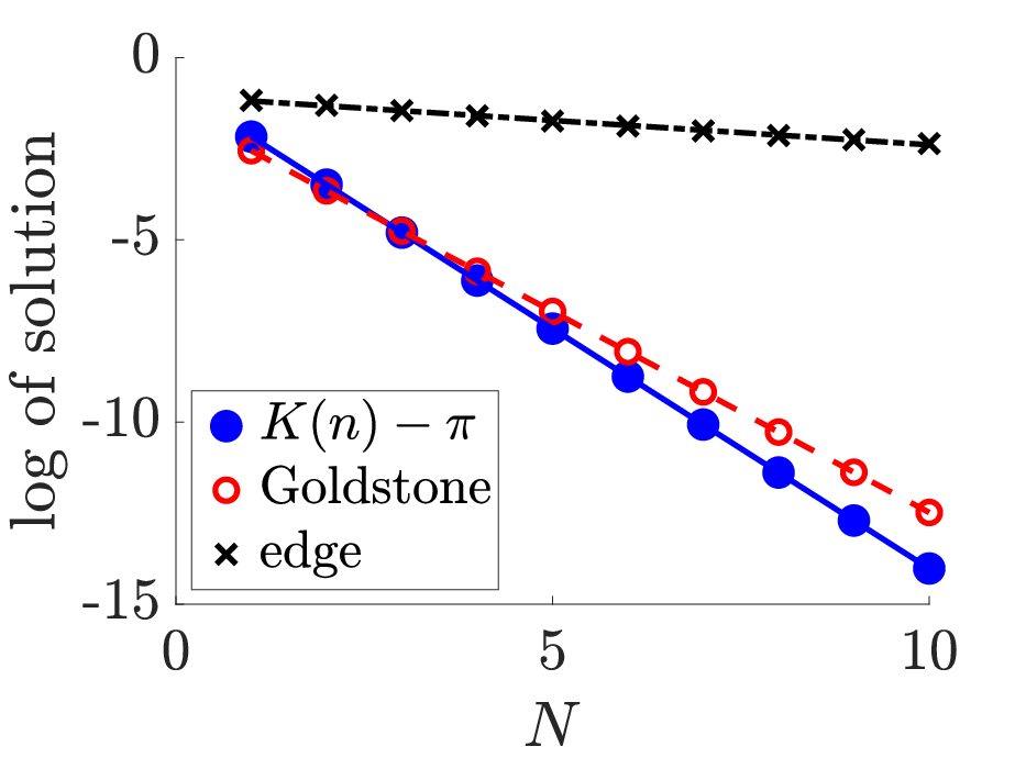
We can compare the eigenvalues obtained from numerical computation with those predicted by Corollary 1. The left panel of Fig. 7 plots the log of the relative error of the two Goldstone eigenvalues vs. the separation distance ; the value for computed with MATLAB from the linearization around the numerically computed kink-antikink solution is used as the true value of . The slope of the least square linear regression line suggests that this error is order . The right panel of Fig. 7 plots the log of the relative error of the two Goldstone eigenvalues vs. the coupling parameter . For intermediate values of , the relative error is less than . The error is a minimum for approximately , and increases with increasing and as the continuum limit is approached. (See [39]*Figure 4 for a similar phenomenon which occurs in the error plot for eigenvalues associated with double pulses in DNLS). Since the results of the Theorem 2 are not uniform in , i.e. they hold for sufficiently large once has been chosen, we indeed expect a growth of the relative error for large .
 |
 |
We can obtain similar results for higher order multi-kinks. An example of a three-component multi-kink is shown in the left panel of Fig. 8. We can again compare the eigenvalues obtained from numerical computation with those predicted by Corollary 1. The right panel of Fig. 8 shows the relative error of the eigenvalue computations for the three Goldstone eigenvalues. One can again observe the particularly good agreement of the theory and the computation, especially so for larger values of .
 |
 |
In addition, for the sine-Gordon equation, we can have generalized multi-kink solutions, in which each kink or antikink in the sequence connects two adjacent saddle equilbria (see Remark 2). An example of a kink-kink is shown in Fig. 9. The spectrum is almost identical to that of the kink-antikink with the same parameters in Fig. 6.
 |
 |
Finally, we perform timestepping simulations of the multikink states. The topic of the evolution of a single (primary) kink was touched upon in the work of [26], where dynamical evolution experiments were performed in the case of a single kink with the Goldstone and/or edge modes excited. It was found that a mechanism of resonance of the point spectrum mode harmonics (i.e., , etc., where is the Goldstone or edge eigenvalue) with the continuous spectrum led to nonlinearity-induced power law decay of relevant mode amplitudes. Here, we instead focus on the evolution of the central nodes of the kinks (e.g. nodes and for a kink located at the origin) for the realm of multi-wave, kink-antikink structures. For a timestepping scheme, since the spatial component is already discretized, we use a symplectic and symmetric implicit Runge-Kutta method [17], as suggested in [13, Section 2.5], to preserve the symplectic structure of the Hamiltonian equation Eq. 1. Specifically, we use the MATLAB implementation of the irk2 scheme of order 12 from [16]. For boundary conditions, we use the discrete analogue of Neumann boundary conditions.
For a kink-antikink constructed from two intersite kinks, the pair of Goldstone mode eigenfunctions suggests that there will be two corresponding normal modes of oscillations for the central nodes of the two kinks: an in-phase mode and an out-of-phase mode. These can be seen in the left and right columns of Fig. 10. In addition, we plot the energy of the solution as evolves (Fig. 10, bottom row). The relative deviation of the energy from its initial value is less than over the time interval of the simulation. There will similarly be two normal modes corresponding to the pair of edge mode eigenfunctions. These panels are representative of the possible in- and out-of-phase motion of the multiple coherent structures.
 |
 |
 |
 |
We can similarly construct a kink-antikink from two onsite kink structures (Fig. 11, top left). The spectrum corresponding to this solution is shown in the top right panel of Fig. 11, in which we see the split Goldstone modes on the real axis, confirming the instability of this bound state. The corresponding Goldstone eigenfunctions are shown in the bottom left panel of Fig. 11. Finally, we perform timestepping experiments for perturbations of this kink-antikink. If we perturb the two central nodes (both of which have values = 0) by a small amount, the solution develops oscillatory behavior about the neutrally stable intersite kink-antikink (Fig. 11, bottom). The solution departs from the corresponding energy maximum and performs oscillations around the nearby energy minimum, namely the stable intersite kink-antikink state. The energy is again very well conserved as evolves (Fig. 11), with a relative deviation from its initial value of less than . We note that for timestepping simulations on long time intervals, energy is very well conserved until boundary effects come into play. For and grid points, these boundary effects occur at approximately and , respectively; enlarging the spatial grid delays these boundary effects.
 |
 |
 |
 |
 |
 |
5. Conclusions and future challenges
In this paper, we used Lin’s method to construct multi-kink solutions to the discrete Klein-Gordon equation by splicing together an alternating sequence of kink and antikink solutions with small amplitude remainders. These solutions exist as long as the distances between adjacent kinks and antikinks are sufficiently large. We then used Lin’s method again to reduce the eigenvalue problem for multi-kinks to an effective, low-dimensional matrix eigenvalue equation. This matrix equation is different for each eigenvalue of the primary kink, and we find that for an -component multi-kink, there are eigenvalues near each eigenvalue of the primary kink. Most notably, if the spectrum of the primary kink is imaginary, the spectrum of a multi-kink constructed from these primary kinks can be shown through this explicit calculation to be imaginary as well. These eigenvalues can be computed numerically, and the result is in good agreement with the theory; this approach explicitly illustrates the spectral stability of these multi-soliton solutions.
Further avenues of research include exploring multi-kinks in other models. One such model is the Ablowitz-Ladik type discretization of the model (AL-) [27]
| (28) |
which has an exact static kink solution , where and is arbitrary. Another is an alternative discretization of the sine-Gordon equation [3]
| (29) |
which has an exact static kink solution
| (30) |
where is defined implicitly by
| (31) |
Here, is the lattice spacing, which is connected to our parameter via , while denotes the kink’s speed. Although we do not expect these equations to have kink-antikink equilibrium solutions, since the stable and unstable manifolds of the two equilibria do not intersect transversely, we expect that a kink-antikink state will be an approximate equilibrium solution. We may then be able to explain the time evolution of the kink-antikink dynamics in terms of interactions between their exponentially decaying tails. In this context, it would be interesting to explore the potential mathematical relevance of the corresponding spectral calculation. While we have already mentioned that similar findings to the ones presented herein are applicable to other Klein-Gordon models, such as, e.g., the discrete model, it would be of interest to study such ideas in more complex model variants such as the sine lattice (SL) studied in the work of [45]. Generalizing such ideas to the context of higher-dimensional Klein-Gordon models where the kinks are typically also dynamically robust would be another direction of interest. We could also explore the time evolution using initial conditions which have the same asymptotics at as a multi-kink. Finally, it remains open to explore whether similar techniques can be used to study multi-site breathers in discrete Klein-Gordon lattices.
Appendix A Proof of Theorem 1
The proof is an adaptation of the proofs of Theorems 1 and 3 in [39]. First, we rewrite the system as a fixed point problem. Expanding in a Taylor series about , we get
| (32) |
where with and . Since is odd, is even, thus , and equation Eq. 32 becomes
| (33) |
Since the pieces in the ansatz Eq. 13 must match at their endpoints, we obtain the following system of equations for the remainder functions
| (34) | ||||
| (35) | ||||
| (36) |
Let be the evolution operators for the linear difference equation
By the stable manifold theorem, for and for , thus . Since are hyperbolic fixed points, we can decompose the evolution operator in exponential dichotomies on by [39]*Lemma 2. The proof then follows that of [39]*Theorems 1 and 3. Briefly, we write equation Eq. 34 in fixed-point form using the discrete variation of constants formula together with projections on the stable and unstable subspaces of the exponential dichotomy. As long as is sufficiently large, we use the implicit function theorem to solve for the remainder functions as well as the matching conditions Eq. 35 and Eq. 36. Since and intersect transversely, we have the decomposition , thus, as in the proof of [39]*Theorem 3, solving Eq. 36 does not involve jump conditions. The estimates Eq. 16 follow from the proof of [39]*Theorem 3 (see in particular [39]*Lemma 4).
Appendix B Proof of Theorem 2
For the multi-kink solution , we will take an ansatz which is a piecewise perturbation of . (This ansatz is suggested in [42]*Section 7). Let
| (37) |
where , , and . Substituting this into Eq. 17 and simplifying using Eq. 18, the eigenvalue problem becomes
| (38) | ||||
where
| (39) |
and we used the fact that from the previous section. Using Eq. 20, we rewrite Eq. 38 as
| (40) |
In addition to solving Eq. 40, the eigenfunction must satisfy matching conditions at and . Thus the system of equations we need to solve is
| (41) | ||||
where
| (42) |
Let be the evolution operator for the variational equation
| (43) |
Since we have the exponential decay Eq. 21, by [39]*Lemma 2, we can decompose the evolution operator in exponential dichotomies on . In particular, we have the estimates
| (44) | ||||||
for the evolution operator on the stable and unstable subspaces of the exponential dichotomy. Furthermore, letting be the stable and unstable eigenspaces of , and the corresponding eigenprojections, we have the decay rates
| (45) |
where are the stable and unstable projections for the exponential dichotomy. We note that the decay rates in Eq. 44 involve the eigenvalues for the matrix , whereas those from Eq. 45 come from Eq. 21.
The variational equation Eq. 43 has a bounded solution , and the adjoint variational equation
| (46) |
has a bounded solution
| (47) |
which is orthogonal to . By the stable manifold theorem,
| (48) | ||||
As in [39, 42], we will not in general be able to solve the system Eq. 41. Instead, since , we relax the third equation in Eq. 41 to obtain the system of equations
| (49) | ||||
Using Lin’s method, we will be able to find a unique solution to this system, but this solution will generically have jumps at in the direction of the adjoint solution . A solution to Eq. 49 is therefore an eigenfunction if and only if the jump conditions
| (50) |
are satisfied. Since , we have the same estimates for as we do for in Eq. 16. The terms in Eq. 49 are the same as in [39], with the addition of a term of the form . To estimate that term, we combine the estimates Eq. 16 and Eq. 48. For the interior pieces, we have
where in the last step we used the fact that is fixed (it depends only on ), as are the distances . The constant will be larger as decreases, which occurs as the eigenvalue gets closer to the continuous spectrum boundary. The estimate for is similar, and the estimates for the two exterior pieces are stronger. Thus we have the two uniform estimates
| (51) | |||
The proof then follows as in [39, 42]. First, we write equation Eq. 38 as a fixed point problem using the discrete variation of constants formula together with projections on the stable and unstable subspaces of the exponential dichotomy. Let be small, and choose sufficiently large so that . Define the spaces
Then for
the fixed point equations for the eigenvalue problem are
where , and the sums are defined to be if the upper index is smaller than the lower index. We now follow the procedure in the proof of [39]*Theorem 2 and invert the system Eq. 49 in the following steps. First, we solve for the remainder functions in the fixed point equations. Then, we use the second equation in Eq. 49 to solve for the initial conditions . Finally, we use the third equation in Eq. 49 to solve for the . The procedure is identical to that in the proof of [39]*Theorem 2, with both and replaced by , replaced by , and the presence of additional terms of the form , which will be small using the second estimate in Eq. 51 and will therefore be incorporated into the remainder term. Thus, we obtain a unique solution to Eq. 36 which generically has jumps in the direction of . These jumps are given by
| (52) |
where is the Melnikov sum
and the remainder term has uniform bound
| (53) |
For the terms in the Melnikov sum,
thus it follows that
| (54) |
which is always positive. It follows from Eq. 45 that
Substituting these into Eq. 52, we have
where the bound on the remainder term is unchanged. Since and have opposite signs, this simplifies to
Let
Using equation Eq. 47,
which we substitute above to obtain
| (55) |
The can be simplified further based on symmetries of the eigenfunction . For even, intersite eigenfunctions, , thus we have
| (56) |
For odd, intersite eigenfunctions, , and so
| (57) |
This can be written as the matrix equation
| (58) |
where is defined by Eq. 25, which has a nontrivial solution if and only if
| (59) |
Let be the eigenvalues of , which are real since is symmetric. They are also distinct by [22]*Corollary 2.2.7, since the eigenvalue problem is equivalent to the Sturm-Liouville difference equation with Dirichlet boundary conditions
where , , is the forward difference operator and is the backward difference operator .
Following the proof of [39]*Theorem 5, we can use the implicit function theorem to solve for to get the solutions
Since , , and must be real, for sufficiently small . The corresponding eigenvalues are , which are on the imaginary axis.
Acknowledgments
This material is based upon work supported by the U.S. National Science Foundation under the RTG grant DMS-1840260 (R.P. and A.A.) and DMS-1809074 (P.G.K.).
References
- [1] (2003) A new barrier to the existence of moving kinks in Frenkel–Kontorova lattices. Physica D: Nonlinear Phenomena 186. Cited by: §1.
- [2] (2000) Being stable and discrete. Physica D: Nonlinear Phenomena 135 (3-4), pp. 212–232 (en). External Links: ISSN 01672789 Cited by: §2, §4.
- [3] (2008) Exceptional discretizations of the sine-gordon equation. Physical Review E 77 (3), pp. 036601. External Links: Link Cited by: §5.
- [4] (1998) Nonlinear dynamics of the Frenkel–Kontorova model. Physics Reports 306 (1-2), pp. 1–108 (en). External Links: ISSN 03701573 Cited by: §1, §1.
- [5] (2004) The Frenkel-Kontorova Model. Springer Berlin Heidelberg, Berlin, Heidelberg. Cited by: §1, §1.
- [6] (1996) Breather mobility in discrete nonlinear lattices. Phys. Rev. Lett. 77, pp. 4776–4779. External Links: Link Cited by: §1.
- [7] (2014) sine-Gordon equation: from discrete to continuum. pp. 31–57. Cited by: §1, §1, §2.
- [8] (2009) Discrete breathers in a forced-damped array of coupled pendula: modeling, computation, and experiment. Phys. Rev. Lett. 102, pp. 224101. External Links: Link Cited by: §1.
- [9] (2011) Multibreather and vortex breather stability in Klein-Gordon lattices: equivalence between two different approaches. International Journal of Bifurcation and Chaos 21 (08), pp. 2161–2177. Cited by: §1.
- [10] (2019) A dynamical perspective on the model. 1 edition, Nonlinear Systems and Complexity, Springer International Publishing. External Links: ISBN 978-3030118389 Cited by: §1.
- [11] (2006) Physics of solitons. 1 edition, Cambridge University Press. Cited by: §1.
- [12] (1982) Solitons and nonlinear wave equations. 1 edition, Academic Press. Cited by: §1.
- [13] (1997) Sympletic finite difference approximations of the nonlinear Klein-Gordon equation. SIAM Journal on Numerical Analysis 34 (5), pp. 1742–1760. External Links: ISSN 0036-1429, 1095-7170 Cited by: §4.
- [14] (2008) Discrete breathers — advances in theory and applications. Physics Reports 467 (1), pp. 1–116. External Links: ISSN 0370-1573, Link Cited by: §1.
- [15] (1998) Josephson-junction ladder: a benchmark for nonlinear concepts. Physica D: Nonlinear Phenomena 113 (2), pp. 387–396. External Links: ISSN 0167-2789, Link Cited by: §1.
- [16] (2003) GniCodes — Matlab programs for geometric numerical integration. In Frontiers in numerical analysis, J. F. Blowey, A. W. Craig, and T. Shardlow (Eds.), pp. 199–240 (en). External Links: Link Cited by: §4.
- [17] (2006) Geometric numerical integration. Springer Series in Computational Mathematics, Vol. 31, Springer-Verlag, Berlin/Heidelberg (en). External Links: ISBN 9783540306634, Link Cited by: §4.
- [18] (1988) Solitons in conducting polymers. Reviews of Modern Physics 60 (3), pp. 781–850 (en). External Links: ISSN 0034-6861 Cited by: §1.
- [19] (2006) Normal form for travelling kinks in discrete Klein–Gordon lattices. Physica D: Nonlinear Phenomena 216. Cited by: §1.
- [20] (2013) Sine–Gordon solitons, kinks and breathers as physical models of nonlinear excitations in living cellular structures. Technical report Journal of Geometry and Symmetry in Physics. Cited by: §1.
- [21] (2014) The sine-Gordon model and its applications: from pendula and Josephson junctions to gravity and high-energy physics. 1 edition, Nonlinear Systems and Complexity 10, Springer International Publishing. External Links: ISBN 978-3-319-06721-6,978-3-319-06722-3 Cited by: §1, §1, §1.
- [22] (1995) Second-order Sturm-Liouville difference equations and orthogonal polynomials. American Mathematical Society. External Links: ISBN 082180359X, Link Cited by: Appendix B.
- [23] (2001) Stability of multiple pulses in discrete systems. Physical Review E 63 (3). Cited by: §1.
- [24] (2001) Stability of waves in discrete systems. Nonlinearity 14 (3), pp. 533–566. Cited by: §2.
- [25] (2005) Global existence in infinite lattices of nonlinear oscillators: the discrete Klein-Gordon equation. Glasgow Mathematical Journal 48. Cited by: §1.
- [26] (2000) Dynamics of lattice kinks. Physica D: Nonlinear Phenomena 142 (1-2), pp. 113–152 (en). External Links: ISSN 01672789, Link Cited by: §1, §2, §2, §2, §2, §4, §4, §4.
- [27] (2003) On a class of discretizations of Hamiltonian nonlinear partial differential equations. Physica D: Nonlinear Phenomena 183 (1-2), pp. 68–86 (en). External Links: ISSN 01672789 Cited by: §5.
- [28] (2009) The discrete nonlinear Schrödinger equation. Springer Berlin Heidelberg. Cited by: §1.
- [29] (1989) Dynamics of solitons in nearly integrable systems. Rev. Mod. Phys. 61, pp. 763–915. Cited by: §1.
- [30] (1998) Internal modes of solitary waves. Phys. Rev. Lett. 80, pp. 5032–5035. External Links: Link Cited by: §2.
- [31] (2000) Lin’s method for discrete dynamical systems. Journal of Difference Equations and Applications 6 (5), pp. 577–623. Cited by: §1, §3.
- [32] (2008) Asymptotics for kink propagation in the discrete Sine-Gordon equation. Physica D: Nonlinear Phenomena 237. Cited by: §1.
- [33] (2011) Some numerical results on motion of kinks in some model of dna torsional dynamics. Communications in Applied and Industrial Mathematics 0 (0). External Links: ISSN 20380909 Cited by: §1.
- [34] (1990) Using Melnikov’s method to solve Silnikov’s problems. Proceedings of the Royal Society of Edinburgh: Section A Mathematics 116 (3-4), pp. 295–325. Cited by: §1.
- [35] (2008) Lin’s method. Scholarpedia 3 (9), pp. 6972. External Links: Link Cited by: §1.
- [36] (1979) An effective lagrangian for solitons. Nuclear Physics B 150, pp. 397–412. External Links: ISSN 0550-3213, Link Cited by: §4.
- [37] (2000) Solitons and the inverse scattering transform. 1 edition, SIAM Studies in Applied Mathematics, No. 4, Society for Industrial Mathematics. External Links: ISBN 9780898714777,089871477X Cited by: §1.
- [38] (2021) Multi-pulse solitary waves in a fourth-order nonlinear Schrödinger equation. Physica D: Nonlinear Phenomena 422, pp. 132890. External Links: ISSN 0167-2789, Link Cited by: §1.
- [39] (2020) Existence and spectral stability of multi-pulses in discrete Hamiltonian lattice systems. Physica D: Nonlinear Phenomena 408, pp. 132414 (en). External Links: ISSN 01672789 Cited by: Appendix A, Appendix A, Appendix B, Appendix B, Appendix B, Appendix B, Appendix B, Appendix B, §1, §1, §2, §3, §4.
- [40] (2012) Multi-site breathers in klein–gordon lattices: stability, resonances and bifurcations. Nonlinearity 25 (12), pp. 3423–3451. External Links: Link Cited by: §1.
- [41] (1984) Kink dynamics in the highly discrete sine-Gordon system. Physica D 14 (1), pp. 88–102. Cited by: §1, §1.
- [42] (1998) Stability of multiple-pulse solutions. Transactions of the American Mathematical Society 350 (02), pp. 429–473. Cited by: Appendix B, Appendix B, Appendix B, §1, §3.
- [43] (1969) A nonlinear klein-gordon equation. American Journal of Physics 37 (1), pp. 52–61. Cited by: §1.
- [44] (1987) Nonexistence of small-amplitude breather solutions in theory. Phys. Rev. Lett. 58, pp. 747–750. External Links: Link Cited by: §1.
- [45] (1986) A sine-lattice (sine-form discrete Sine-Gordon) equation–one-and two-kink solutions and physical models–. Journal of the Physical Society of Japan 55. Cited by: §5.
- [46] (1992) Dynamics of sine-Gordon solitons in the annular Josephson junction. Phys. Rev. Lett. 69, pp. 1815–1818. External Links: Link Cited by: §1.
- [47] (1998) Nonlinear physics of DNA. Wiley series in nonlinear science, John Wiley Sons, Chichester ; New York. External Links: ISBN 9780471978244 Cited by: §1.
- [48] (1983) Soliton excitations in deoxyribonucleic acid (dna) double helices. Phys. Rev. A 27, pp. 2120–2125. Cited by: §1.