Characterizing the Gap Between Actor-Critic and Policy Gradient

Consider the two standard actor-critic objectives:

The actor objective is an approximation of Eq. 6 using a parameterized critic $\mathbf{q}_{\phi}$ in place of $\mathbf{q}_{\theta}$. To learn a critic that estimates the policy’s $Q$-values, the critic objective minimizes the Bellman residual weighted by a state-action distribution $\mathbf{d}$, which is assumed to have full support. From a practical standpoint, $\mathbf{d}$ is equivalent to a (fixed) replay buffer distribution from which the state-actions are sampled. An on-policy assumption is equivalent to setting $\mathbf{d}=\mathbf{d}_{\theta}$, the current policy’s stationary distribution. Given these objectives, the partial derivatives are⁴⁴ 4 Unlike Eq. 8, we use $\partial_{\theta}$ instead of $\nabla_{\theta}$ when the quantity in question depends on both $\bm{\theta}$ and $\bm{\phi}$.

where $\bm{\delta}_{\theta,\phi}:=\mathbf{r}-\Psi_{\theta}\mathbf{q}_{\phi}$ is the residual of the critic. From this objective perspective, actor-critic (which we refer to as Actor_o-Critic) alternates between ascent on the actor and descent on the critic using their respective gradients⁵⁵ 5 For notational simplicity, we use the same learning rate $\alpha$ for both the actor and the critic even though this is not needed for any of our conclusions.:

As an example, Soft Actor-Critic (Haarnoja et al., 2018a) can be considered as using variants of these updates (with entropy regularization, as shown in Appendix C).

Alternatively, one can consider $\nabla_{\theta}^{\phi}J$ in Eq. 9 which applies the critic after the gradient is derived. A2C (Mnih et al., 2016) is an example of such an approach. A key observation is that $\nabla^{\phi}_{\theta}J$ differs from $\partial_{\theta}J_{\pi}$ (Eq. 12) in terms of the state distribution they consider: $\partial_{\theta}J_{\pi}$ uses the initial state distribution, whereas $\nabla_{\theta}^{\phi}J$ uses the policy’s stationary distribution. Therefore, using $\nabla^{\phi}_{\theta}J$, one can define an alternative actor update

To distinguish this from Actor_o-Critic, we refer to the updates (15)–(16) collectively as Actor_g-Critic (since the actor update is derived from a gradient perspective). In the literature, AC typically refers to what we call Actor_g-Critic (Sutton et al., 2000; Konda and Tsitsiklis, 2000).

Given these two perspectives, we can now show how classical algorithms can simply be interpreted as alternative interplays between the actor and critic updates; see Table 1.

Policy Iteration, for example, alternates between policy evaluation and policy improvement. Policy evaluation corresponds to fully optimizing the critic to becoming the policy’s $Q$-values: $\mathbf{q}_{\phi}\leftarrow\mathbf{q}_{\theta}$. Policy improvement updates the policy to be greedy with respect to its $Q$-values. Since the critic is fully optimized, it is equivalent to a policy that is greedy with respect to the current critic: $\bm{\theta}\leftarrow\bm{\theta}^{*}(\mathbf{q}_{\phi})$. As noted in Section 2, AC methods are typically derived from policy iteration. What is often overlooked, however, is that Actor_o-Critic and Actor_g-Critic present distinct instances of this general framework.

Policy Gradient_g. When the critic is fully optimized for every actor step (i.e., policy evaluation with infinite critic capacity $\mathbf{q}_{\phi}\leftarrow\mathbf{q}_{\theta}$), we have $\nabla_{\theta}^{\phi}J=\nabla_{\theta}J$, which corresponds to the classical policy gradient method (Eq. 8). Note that this is different from Policy Gradient_o, which is defined to be $\partial_{\theta}J_{\pi}$ (Eq. 12) with $\mathbf{q}_{\phi}=\mathbf{q}_{\theta}$ (similar to Actor_o from the objective perspective). The key difference is that Policy Gradient_g uses the the on-policy distribution $d_{{\mathcal{S}},\theta}(s)$ to weight the states, whereas Policy Gradient_o uses the initial state distribution $\mu_{0}(s)$.

Q-Learning. The critic gradient in Eq. 13 is the gradient of the expected squared Bellman residual, which involves double-sampling (Baird, 1995). Therefore, a semi-gradient (Sutton and Barto, 2018, Sec.9.3) is used in practice. If the critic is directly parametrized (i.e., $\mathbf{q}_{\phi}=\bm{\phi}=\mathbf{q}\in\mathbb{R}^{|\mathcal{S}||\mathcal{A}|\times 1}$), the critic update becomes

and $\mathbf{q}^{\prime}:=\mathbf{r}+\gamma P\Pi_{\theta}\mathbf{q}$ is the target value, whose gradient is ignored. When the policy is fully optimized w.r.t. $\mathbf{q}$ (last row of Table 1), $\gamma P\Pi_{\theta}\mathbf{q}$ will choose the maximum next-state value, making $\mathbf{q}^{\prime}$ the usual Q-Learning target. When $D=D_{\theta}$ in Eq. 17, $\mathbf{q}$ is updated according to on-policy experience, yielding the on-policy Q-Learning algorithm.

To characterize the gap from the objective perspective, consider the difference between the policy objective (6) and the actor objective (10) in $\text{Actor}_{o}$-Critic. Using the dual formulation of the policy objective (7), the difference is:

where the first equality replaces $(1-\gamma)\bm{\mu}_{0}^{\top}\Pi_{\theta}$ with $\mathbf{d}_{\theta}^{\top}\Psi_{\theta}$ using Eq. 3. Therefore, the difference is $\mathbf{d}^{\top}_{\theta}\bm{\delta}_{\theta,\phi}$, which is the inner product between the stationary distribution of $\bm{\pi}_{\theta}$ and the on-policy residual of the critic $\mathbf{q}_{\phi}$ under $\bm{\pi}_{\theta}$. This also implies that the difference between the Actor_o-gradient, $\partial_{\theta}J_{\pi}$, and the policy gradient, $\nabla_{\theta}J$, is exactly equal to $\partial_{\theta}(\mathbf{d}_{\theta}^{\top}\bm{\delta}_{\theta,\phi})$, which we analyze below.

Note that by the product rule,

where $\mathbf{d}^{\prime}_{\theta}$ and $\bm{\delta}^{\prime}_{\theta,\phi}$ are treated as being independent of the policy parameter $\bm{\theta}$ (i.e., without computing gradients). Then the policy gradient can be expressed as

The first term is given by Eq. 12, and the second term is

To further simplify, one can use the $\log$ derivative trick (i.e., $\nabla_{\theta}\pi_{\theta}=\pi_{\theta}\nabla_{\theta}\log\pi_{\theta}$) so that

Note that these two terms can be combined, using the recursive definition of $\mathbf{d}_{\theta}$ (Eq. 3), as

which is equivalent to $\nabla_{\theta}^{\phi}J$ in Eq. 9. This is somewhat surprising. Now one can see that $\nabla_{\theta}^{\phi}J$ is in fact maximizing $J_{\pi}+(\mathbf{d}^{\prime}_{\theta})^{\top}\bm{\delta}_{\theta,\phi}$, which is nearly identical to the policy objective except that it ignores the last term of (21), $\partial_{\theta}(\mathbf{d}^{\top}_{\theta}\bm{\delta}^{\prime}_{\theta,\phi})$ (i.e., the dependence of $\mathbf{d}_{\theta}$ on $\bm{\theta}$). The following theorem summarizes the gap between policy gradient and actor gradients.

We will discuss how to estimate $\partial_{\theta}(\mathbf{d}^{\top}_{\theta}\bm{\delta}^{\prime}_{\theta,\phi})$ in Section 4.3.

Additional insight is gained by considering the difference between AC and PG from the gradient perspective. This section provides a different and possibly more direct way to correct $\nabla_{\theta}^{\phi}J$, where the critic replaces the on-policy values after the policy gradient is derived. Recall the policy gradient and $\nabla_{\theta}^{\phi}J$, and observe that they can be rewritten respectively as (see Appendix A):

Clearly, $\nabla^{\phi}_{\theta}J\neq\nabla_{\theta}J$ unless $\mathbf{q}_{\phi}$ satisfies specific conditions (Sutton et al., 2000, Thm.2). Their difference is:

To further simplify, consider the following theorem.

All proofs can be found in Appendix B. Using this theorem, one can see that Eq. 28 is in fact

which provides an alternative way to prove the gap between PG and AC as shown in Theorem 1.

Theorem 2 in itself can be useful in some other contexts. A related result can be found in Morimura et al., 2010, which is a recursive form for the derivative of the log stationary distribution. Our theorem here provides a direct and explicit form for the derivative of the distribution.

The key insight from both Sections 4.1 and 4.2 is that bridging the gap between AC and PG requires the computation of $\partial_{\theta}(\mathbf{d}_{\theta}^{\top}\bm{\delta}^{\prime}_{\theta,\phi})$. Our next main contribution is to develop a practical strategy to estimate this gap, which will reduce the bias introduced by the critic and bring the actor update in AC closer to the true policy gradient. This results in a new AC framework we call Residual Actor-Critic.

To develop a practical estimator, first note that $\mathbf{d}_{\theta}^{\top}\bm{\delta}^{\prime}_{\theta,\phi}$ can be treated as a dual policy objective (Eq. 7), where the environment’s reward $\mathbf{r}$ is replaced by the residual $\bm{\delta}^{\prime}_{\theta,\phi}$ of the critic $\mathbf{q}_{\phi}$. The corresponding primal objective is

where $\mathbf{w}_{\theta}=\sum_{i=0}^{\infty}(\gamma P\Pi_{\theta})^{i}\bm{\delta}^{\prime}_{\theta,\phi}$ is the on-policy $Q$-value associated with the residual reward. The gradient of (30) is precisely the desired correction, $\partial_{\theta}(\mathbf{d}_{\theta}^{\top}\bm{\delta}^{\prime}_{\theta,\phi})$. Computing its gradient requires $\mathbf{w}_{\theta}$, which can be approximated by introducing a residual-critic (or res-critic) $\mathbf{w}_{\psi}$ with parameters $\bm{\psi}$. Concretely, the res-critic solves the following problem:

Once we have a relatively accurate res-critic $\mathbf{w}_{\psi}$, we apply the PG_g method (see Table 1) and use the following to approximate $\partial_{\theta}(\mathbf{d}_{\theta}^{\top}\bm{\delta}^{\prime}_{\theta,\phi})$

Combining these update rules for the actor and res-critic with the standard AC update rules results in our Residual Actor-Critic (Res-AC) framework, which can be summarized as follows:

To understand the correction term $\nabla_{\theta}^{\psi}J_{\delta}$ intuitively, note that the residual reward $\bm{\delta}^{\prime}_{\theta,\phi}$ is signed. For an $(s,a)$ with $\delta^{\prime}_{\theta,\phi}(s,a)>0$, we have $q_{\phi}(s,a)<r(s,a)+\gamma\mathbb{E}[q_{\phi}(\widetilde{s},\widetilde{a})]$, and the agent is incentivized to visit the underestimated region. On the other hand, if $\delta^{\prime}_{\theta,\phi}(s,a)<0$, the agent is discouraged to visit the overestimated location.

Res-AC is a generic framework that can be combined with different AC-based algorithms. In Appendix C and in the experiments, we show that Soft Actor-Critic (SAC) (Haarnoja et al., 2018a) can be enhanced with a res-critic and the resultant Res-SAC method improves over the original SAC.

Actor-critic methods can be considered as a two-player general-sum game, where the actor and critic are the players and the objectives (Eqs. 10 and 11) are their respective utility/cost functions. More specifically, one can treat actor-critic as a Stackelberg game in which there is a leader who moves first and a follower who moves subsequently (Sinha et al., 2017). By treating the actor as the leader, Stackelberg Actor-Critic (Stack-AC) solves the following

A key distinction from the original AC is that the actor is now aware of the critic’s goal. Given that in the ideal case $\mathbf{q}$ is implicitly a function of $\bm{\theta}$ (i.e., policy evaluation), one may differentiate through $\mathbf{q}$ to obtain the following Stackelberg gradient⁶⁶ 6 It is the total derivative from the implicit function theorem. (Fiez et al., 2020)

The second order derivative $\partial_{q}^{2}J_{q}$ can be computed, based on the critic objective Eq. 11, as

which is invertible under 1, hence the Stackelberg gradient is well-defined. However, it is unclear what this gradient achieves in the AC setting. We show, in the following theorem, that the Stackelberg gradient is in fact the policy gradient of the cumulative reward objective (6).

This indicates that, under some conditions, one can compute the gradient of the objective correction in Eq. 19 using $(\partial_{\theta}\partial_{q}J_{q})^{\top}(\partial_{q}^{2}J_{q})^{-1}(\partial_{q}J_{\pi})$.

As discussed earlier in Section 3.3, it is common to use a semi-gradient update for the critic to address the double sampling issue. This section shows that, surprisingly, the Stackelberg gradient remains the true policy gradient even when using semi-gradient for the critic.

From the semi-gradient (18), the semi-Hessian is

Compared to Eq. 39, the derivative does not go through the next-state values so $\Psi_{\theta}$ is now replaced by the identity matrix. Additionally, the actor objective can be reformulated using Eq. 3 as

Thus the semi-derivative is

Then the Stackelberg gradient based on semi-critic-gradient is given by

which again corresponds to the true policy gradient.

The update rules for Stack-AC are summarized as follows

where the Stackelberg gradient $\mathbf{g}^{\text{semi}}_{S,\theta}$ can be approximated using sample-based estimate for each term in Eq. 43. Although Eq. 43 requires an inverse-Hessian-vector product and a Jacobian-vector product, they can be efficiently carried out or approximated using standard libraries (Fiez et al., 2020). Following Fiez et al., 2020, we use a regularized version where $(\partial_{q}^{\text{semi}})^{2}J_{q}$ is replaced by $(\partial_{q}^{\text{semi}})^{2}J_{q}+\eta I$ with $\eta=0.5$ in our experiments (Section 6). This can ensure invertibility and stabilize learning.

There is one caveat when estimating $\partial_{\theta}\partial_{q}^{\text{semi}}J_{q}$ in $\mathbf{g}_{S,\theta}^{\text{semi}}$ from samples. The critic objective can be written as $J_{q}=\frac{1}{2}\mathbf{d}_{\theta}^{\top}\bm{\delta}^{2}_{\theta,\phi}$. $\partial_{q}^{\text{semi}}J_{q}$ can be estimated using a batch $\mathcal{B}$ of samples drawn from $\mathbf{d}_{\theta}$. However, $\partial_{\theta}\partial_{q}^{\text{semi}}J_{q}=\partial_{\theta}(-D_{\theta}\bm{\delta}_{\theta,\phi})$ is now difficult to estimate because we cannot take derivative of $\bm{\theta}$ through the batch $\mathcal{B}$, which represents the derivative through $D_{\theta}$. As a result, a sample-based estimate of $\partial_{\theta}\partial_{q}^{\text{semi}}J_{q}$ is only estimating $\partial_{\theta}(-D^{\prime}_{\theta}\bm{\delta}_{\theta,\phi})$, where $D^{\prime}_{\theta}$ is consider a fixed distribution unrelated to $\bm{\theta}$.

To summarize, the Stackelberg policy gradient can close the gap between AC and PG under certain conditions, even with semi-gradient updates. Despite being biased when approximated using samples, we will show in our experiments that Stack-AC can work reasonably well in practice.

In the FourRoom domain, we use a tabular parameterization $\mathbf{q}$ for the critic and a softmax tabular actor $\bm{\pi}$. All our AC methods collect data from the environment and compute updates for the actor and critic (and res-critic for Res-AC) using this data. We train each algorithm with three different random seeds, and we plot the return of the current policy after each episode, where every episode has a fixed length of 300 environment steps (Fig. 1). The curves correspond to the mean return and the shaded region to one standard deviation over the three trials.

Res-AC enjoys improved sample-efficiency as well as final performance when compared to all other methods. Stack-AC and Actor_o-Critic achieve a lower final performance than Res-SAC, and they perform comparably to each other. Actor_g-Critic achieves a similar final return as Res-AC, but requires over 150,000 additional environment steps. The relatively poor performance of Stack-AC is not surprising since the sample-based estimate of $\partial_{\theta}\partial_{q}^{\text{semi}}J_{q}$ is inaccurate, as discussed in Section 5.3. In contrast, even though Res-AC introduces an additional problem of using a res-critic to learn the on-policy return with $\bm{\delta}^{\prime}_{\theta,\phi}$ as reward, the res-critic significantly accelerates the improvement of the actor.

To gain further understanding of the residual critic, Fig. 2 plots the predictions of the critic and res-critic for Res-AC on the FourRoom domain. The sum of the critic and res-critic approximates the true return better than the critic alone throughout training. This shows that the res-critic can correct the bias introduced by the critic in policy gradient empirically.

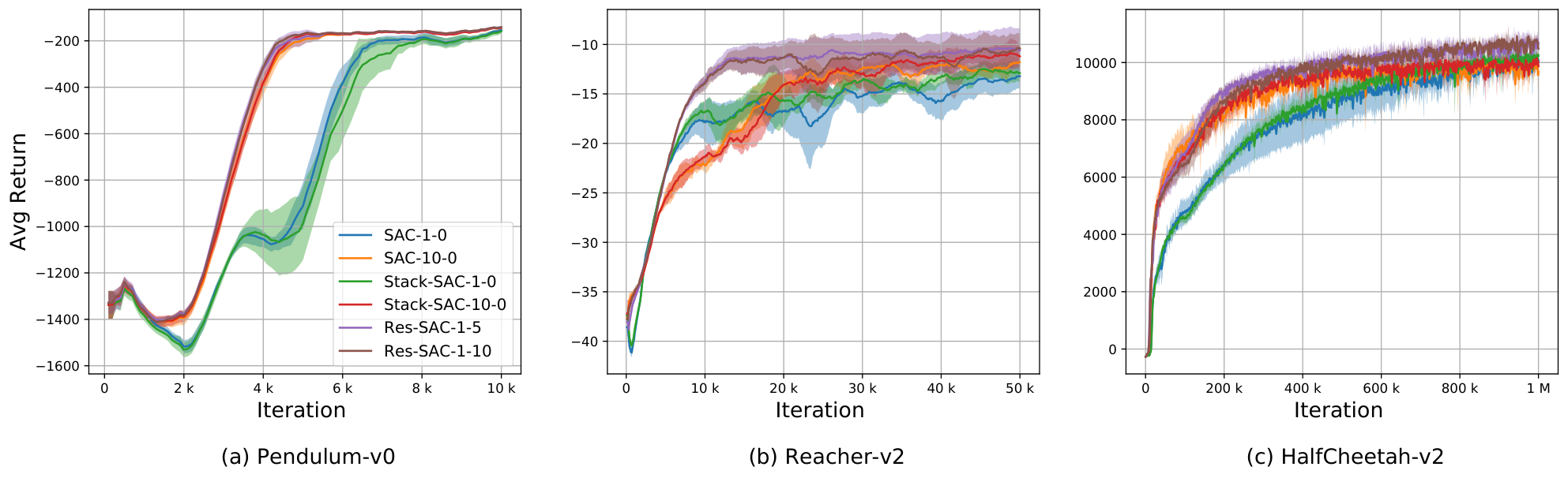
We compare SAC to Res-SAC and Stack-AC on Pendulum-v0, Reacher-v2, and HalfCheetah-v2. We additionally introduce an update schedule for an algorithm $Algo$ labelled as “$Algo$-$x$-$y$”, where $x$ and $y$ are the number of gradient updates applied to the critic and res-critic, respectively, for each actor gradient update. For example, SAC-10-0 refers to SAC with 10 critic gradient updates per actor update. (Note that the number of res-critic updates here is 0 since SAC does not use a res-critic.) In the original SAC algorithm, only one critic update is performed per actor update. Our decision to optionally perform multiple gradient updates for the critic / res-critic is guided by the intuition that a more accurate critic / res-critic would benefit the gradient updates to the policy.

For SAC, Stack-SAC, and Res-SAC, we use the hyper-parameters used in Haarnoja et al., 2018b on all environments. Stack-SAC includes an additional regularization parameter $\eta$, introduced in Section 5.3, which we set to 0.5 for all experiments. Even though the theoretical properties of Stackelberg gradient may not hold for continuous environments (Theorem 3), we can still implement it for our experiments and investigate its performance. The performance of Res-SAC is dependent on clipping the residual that is used as the reward for the res-critic. Concretely, for a clip value $c>0$, the reward for updating the res-critic is computed as $\text{clip}(\bm{\delta}_{\theta,\phi},-c,c)$. Without clipping, large values of the critic’s residual can make training the res-critic unstable. Additional discussion on the choice of clipping value can be found in Section D.2.2.

The results in Fig. 3 show that Res-SAC is consistently more sample-efficient than the other methods and even achieves higher asymptotic performance on Reacher-v2. Applying multiple critic updates per actor-update significantly improves the performance of SAC, as SAC-10-0 consistently outperforms SAC-1-0. The better performance of Res-SAC over SAC-10-0 suggests that bringing the actor update closer to the true policy gradient in theory translates to empirical benefits. In contrast, Stack-SAC performs comparably to SAC – there is not a clear benefit to using the Stack-SAC actor update rule over the standard SAC actor update. This is understandable as 1 does not hold when the critic uses non-linear function approximation.

References

- Baird, (1995) Baird, L. (1995). Residual algorithms: Reinforcement learning with function approximation. In Machine Learning Proceedings 1995, pages 30–37. Elsevier.
- Chou et al., (2017) Chou, P.-W., Maturana, D., and Scherer, S. (2017). Improving stochastic policy gradients in continuous control with deep reinforcement learning using the beta distribution. In International conference on machine learning, pages 834–843. PMLR.
- Dabney et al., (2020) Dabney, W., Kurth-Nelson, Z., Uchida, N., Starkweather, C. K., Hassabis, D., Munos, R., and Botvinick, M. (2020). A distributional code for value in dopamine-based reinforcement learning. Nature, 577(7792):671–675.
- Degris et al., (2012) Degris, T., White, M., and Sutton, R. S. (2012). Off-policy actor-critic. In Proceedings of the 29th International Coference on International Conference on Machine Learning, pages 179–186.
- Fiez et al., (2020) Fiez, T., Chasnov, B., and Ratliff, L. (2020). Implicit learning dynamics in stackelberg games: Equilibria characterization, convergence analysis, and empirical study. In International Conference on Machine Learning (ICML).
- Fujimoto et al., (2018) Fujimoto, S., Hoof, H., and Meger, D. (2018). Addressing function approximation error in actor-critic methods. In International Conference on Machine Learning, pages 1587–1596. PMLR.
- Ghosh et al., (2020) Ghosh, D., Machado, M. C., and Roux, N. L. (2020). An operator view of policy gradient methods. In Advances in Neural Information Processing Systems 33: Annual Conference on Neural Information Processing Systems 2020, NeurIPS 2020, December 6-12, 2020, virtual.
- (8) Haarnoja, T., Zhou, A., Abbeel, P., and Levine, S. (2018a). Soft actor-critic: Off-policy maximum entropy deep reinforcement learning with a stochastic actor. In International Conference on Machine Learning, pages 1861–1870.
- (9) Haarnoja, T., Zhou, A., Hartikainen, K., Tucker, G., Ha, S., Tan, J., Kumar, V., Zhu, H., Gupta, A., Abbeel, P., et al. (2018b). Soft actor-critic algorithms and applications. arXiv preprint arXiv:1812.05905.
- Konda and Tsitsiklis, (2000) Konda, V. R. and Tsitsiklis, J. N. (2000). Actor-critic algorithms. In Advances in neural information processing systems, pages 1008–1014. Citeseer.
- Lillicrap et al., (2016) Lillicrap, T. P., Hunt, J. J., Pritzel, A., Heess, N., Erez, T., Tassa, Y., Silver, D., and Wierstra, D. (2016). Continuous control with deep reinforcement learning. In ICLR.
- Liu et al., (2020) Liu, Y., Swaminathan, A., Agarwal, A., and Brunskill, E. (2020). Off-policy policy gradient with stationary distribution correction. In Uncertainty in Artificial Intelligence, pages 1180–1190. PMLR.
- Maei et al., (2009) Maei, H. R., Szepesvari, C., Bhatnagar, S., Precup, D., Silver, D., and Sutton, R. S. (2009). Convergent temporal-difference learning with arbitrary smooth function approximation. In NIPS, pages 1204–1212.
- Marbach and Tsitsiklis, (2001) Marbach, P. and Tsitsiklis, J. N. (2001). Simulation-based optimization of markov reward processes. IEEE Transactions on Automatic Control, 46(2):191–209.
- Mnih et al., (2016) Mnih, V., Badia, A. P., Mirza, M., Graves, A., Lillicrap, T., Harley, T., Silver, D., and Kavukcuoglu, K. (2016). Asynchronous methods for deep reinforcement learning. In International conference on machine learning, pages 1928–1937.
- Morimura et al., (2010) Morimura, T., Uchibe, E., Yoshimoto, J., Peters, J., and Doya, K. (2010). Derivatives of logarithmic stationary distributions for policy gradient reinforcement learning. Neural computation, 22(2):342–376.
- Nachum et al., (2017) Nachum, O., Norouzi, M., Xu, K., and Schuurmans, D. (2017). Bridging the gap between value and policy based reinforcement learning. In Advances in Neural Information Processing Systems.
- O’Donoghue et al., (2017) O’Donoghue, B., Munos, R., Kavukcuoglu, K., and Mnih, V. (2017). Combining policy gradient and q-learning. In ICLR.
- Peters and Schaal, (2008) Peters, J. and Schaal, S. (2008). Natural actor-critic. Neurocomputing, 71(7-9):1180–1190.
- Puterman, (2014) Puterman, M. L. (2014). Markov decision processes: discrete stochastic dynamic programming. John Wiley & Sons.
- Rajeswaran et al., (2020) Rajeswaran, A., Mordatch, I., and Kumar, V. (2020). A game theoretic framework for model-based reinforcement learning. In International Conference on Machine Learning.
- Schaul et al., (2016) Schaul, T., Quan, J., Antonoglou, I., and Silver, D. (2016). Prioritized experience replay. In ICLR.
- Scherrer, (2010) Scherrer, B. (2010). Should one compute the temporal difference fix point or minimize the bellman residual? the unified oblique projection view. In Proceedings of the 27th International Conference on International Conference on Machine Learning, pages 959–966.
- Schulman et al., (2018) Schulman, J., Chen, X., and Abbeel, P. (2018). Equivalence between policy gradients and soft q-learning. ArXiv:1704.06440. URL.
- (25) Schulman, J., Heess, N., Weber, T., and Abbeel, P. (2015a). Gradient estimation using stochastic computation graphs. In Proceedings of the 28th International Conference on Neural Information Processing Systems-Volume 2, pages 3528–3536.
- (26) Schulman, J., Levine, S., Abbeel, P., Jordan, M., and Moritz, P. (2015b). Trust region policy optimization. In International conference on machine learning, pages 1889–1897. PMLR.
- Schulman et al., (2016) Schulman, J., Moritz, P., Levine, S., Jordan, M., and Abbeel, P. (2016). High-dimensional continuous control using generalized advantage estimation. In ICLR.
- Sherstan et al., (2018) Sherstan, C., Ashley, D. R., Bennett, B., Young, K., White, A., White, M., and Sutton, R. S. (2018). Comparing direct and indirect temporal-difference methods for estimating the variance of the return. In UAI, pages 63–72.
- Sinha et al., (2017) Sinha, A., Malo, P., and Deb, K. (2017). A review on bilevel optimization: from classical to evolutionary approaches and applications. IEEE Transactions on Evolutionary Computation, 22(2):276–295.
- Sun et al., (2011) Sun, Y., Gomez, F., Ring, M., and Schmidhuber, J. (2011). Incremental basis construction from temporal difference error. In Proceedings of the 28th International Conference on International Conference on Machine Learning, pages 481–488.
- Sutton and Barto, (2018) Sutton, R. S. and Barto, A. G. (2018). Reinforcement learning: An introduction. MIT press.
- Sutton et al., (2009) Sutton, R. S., Maei, H. R., Precup, D., Bhatnagar, S., Silver, D., Szepesvári, C., and Wiewiora, E. (2009). Fast gradient-descent methods for temporal-difference learning with linear function approximation. In Proceedings of the 26th Annual International Conference on Machine Learning, pages 993–1000.
- Sutton et al., (2000) Sutton, R. S., McAllester, D. A., Singh, S. P., and Mansour, Y. (2000). Policy gradient methods for reinforcement learning with function approximation. In Advances in neural information processing systems, pages 1057–1063.
- Todorov et al., (2012) Todorov, E., Erez, T., and Tassa, Y. (2012). Mujoco: A physics engine for model-based control. In 2012 IEEE/RSJ International Conference on Intelligent Robots and Systems, pages 5026–5033. IEEE.
- Van Seijen and Sutton, (2013) Van Seijen, H. and Sutton, R. (2013). Planning by prioritized sweeping with small backups. In International Conference on Machine Learning, pages 361–369. PMLR.
- Wang et al., (2007) Wang, T., Bowling, M., and Schuurmans, D. (2007). Dual representations for dynamic programming and reinforcement learning. In 2007 IEEE International Symposium on Approximate Dynamic Programming and Reinforcement Learning, pages 44–51. IEEE.
- Williams, (1992) Williams, R. J. (1992). Simple statistical gradient-following algorithms for connectionist reinforcement learning. In Machine Learning, pages 229–256.
Appendix
Appendix A Notations
For better understanding, this section provides notation conversions for some of the key concepts in the main text beyond matrix-vector notation.
Appendix B Proofs
See 2
Proof.
By the chain rule, we can calculate as