Adaptation of the Tuning Parameter in General Bayesian Inference with Robust Divergence
Abstract
We introduce a novel methodology for robust Bayesian estimation with robust divergence (e.g., density power divergence or -divergence), indexed by tuning parameters. It is well known that the posterior density induced by robust divergence gives highly robust estimators against outliers if the tuning parameter is appropriately and carefully chosen. In a Bayesian framework, one way to find the optimal tuning parameter would be using evidence (marginal likelihood). However, we theoretically and numerically illustrate that evidence induced by the density power divergence does not work to select the optimal tuning parameter since robust divergence is not regarded as a statistical model. To overcome the problems, we treat the exponential of robust divergence as an unnormalisable statistical model, and we estimate the tuning parameter by minimising the Hyvarinen score. We also provide adaptive computational methods based on sequential Monte Carlo (SMC) samplers, enabling us to obtain the optimal tuning parameter and samples from posterior distributions simultaneously. The empirical performance of the proposed method through simulations and an application to real data are also provided.
Keywords: General Bayes; robustness; tuning parameter estimation; density power divergence; sequential Monte Carlo.
1 Introduction
One well-known way to deal with outliers and model misspecification when conducting inference is to use robust divergences. Since the pioneering work of Basu et al., 1998 that proposed density power divergence as an extension of the standard likelihood, some variants of the divergence (Fujisawa and Eguchi, 2008; Cichocki et al., 2011; Ghosh et al., 2017, e.g.) and various statistical methods using robust divergences have been developed. Many robust divergences are indexed by a single tuning parameter that controls the robustness against outliers. If the tuning parameter is set to a smaller value than necessary, the resulting estimator may still be affected by outliers. On the other hand, using an unnecessarily large value for the tuning parameter leads to a loss of statistical efficiency (Basu et al., 1998). Despite the success of the theoretical analysis of properties of statistical methods based on robust divergences, how to adaptively estimate the tuning parameter from the data has often been ignored, with a few exceptions (Warwick and Jones, 2005; Basak et al., 2021) that propose frequentist methods to select the optimal value via asymptotic mean squared errors. There is a growing body of literature on Bayesian approaches using robust divergence. For example, general theory has been considered by (Ghosh and Basu, 2016; Jewson et al., 2018; Nakagawa and Hashimoto, 2020) and some specific applications to statistical models such as linear regression (Hashimoto and Sugasawa, 2020), change point detection (Knoblauch et al., 2018) and Bayesian filtering (Boustati et al., 2020). Nevertheless, a reasonable estimation strategy for the tuning parameter has not been carefully discussed. A natural consideration to find the best tuning parameter in the context of Bayesian statistics will be the use of model evidence or marginal likelihood. However, as we shall illustrate later, evidence is not useful for choosing the tuning parameter since the exponential of robust divergence cannot be directly interpreted as a normalised statistical model.
In this paper, this issue is addressed by taking advantage of ideas from statistical theories for unnormalised statistical models (Hyvärinen, 2005) introducing the Hyvarinen score (H score), which is a finite version of Fisher divergence. Based upon the idea of Hyvärinen, 2005, Dawid et al., 2015; Shao et al., 2019 consider unnormalisable marginal likelihoods, with particular attention to model selection, where such unnormalisability is driven by the improper prior. Our main idea is to regard the exponential of robust divergence as unnormalisable models and employ a posterior distribution driven by the H-score, inspired by Dawid et al., 2015; Shao et al., 2019, as an objective function of . Since our objective function cannot be computed analytically in general, we then take advantage of sequential Monte Carlo (SMC) samplers (Del Moral et al., 2006) within a Robbins-Monro stochastic gradient framework to approximate the objective function, to estimate the optimal tuning parameter and to obtain samples from posterior distributions.
Therefore, our work can be understood as an attempt to fill the current gap between the existing theory of such robust estimation and their practical implementation. Our proposed method has the following advantages over existing studies.
- i)
Unlike existing methods (Warwick and Jones, 2005; Basak et al., 2021), our proposed method does not require a pilot plot. To optimise a tuning parameter, it is necessary to determine a certain value as a pilot estimate. Thus, the estimates may be strongly dependent on the pilot estimate. In addition, such methods often estimate excessively large values of the tuning parameters, given the proportion of outliers in the data. In contrast, our algorithm is stable and statistically efficient since that does not require a pilot estimate.
- ii)
Proposed methods in (Warwick and Jones, 2005; Basak et al., 2021) require an analytical representation of the asymptotic variance that cannot be obtained in general. Compared to such methods, our proposed method does not require such expression, and therefore our method can be applied to rather complex statistical models, which seem difficult to be handled by the previous methods.
- iii)
We take advantage of SMC samplers (Del Moral et al., 2006) in the generalised Bayesian framework (Bissiri et al., 2016) with a gradient-ascent approach to perform parameter inference for the tuning parameter and posterior sampling simultaneously. This is a unique favourable algorithmic characteristic compared to methods that estimate parameters by fixing tuning parameters or by estimating tuning parameters once and then estimating other objects of interest.
Recently, Jewson and Rossell, 2021 has introduced a new Bayesian framework called H-posterior for unnormalisable statistical models based on Fisher divergence, and they have developed model selection criterion via the Laplace approximation of the marginal likelihood. The biggest difference from Jewson and Rossell, 2021 is that we use a natural form of general posterior based on robust divergence, which is widely adopted in the literature (Ghosh and Basu, 2016; Jewson et al., 2018, e.g.), while the form of the posterior distribution in Jewson and Rossell, 2021 is different from ours. As we mentioned, the main contribution of their work is the construction of model selection criteria of the BIC type through the Laplace approximation and the proof of their consistency. On the other hand, our research is about the estimation of tuning parameters and the inference of the posterior distribution, and the main objective is to propose an objective function and a computational method considered suitable for this purpose. In the framework of Generalised Bayesian, some methods that use variational Bayesian inference (Knoblauch et al., 2019; Frazier et al., 2021) have also been proposed. However, instead of computational speed, the approximate distribution obtained does not match the target distribution in the limit, and the method of estimating the tuning parameters is unclear. There is also a need to make some natural but somewhat stronger assumptions than our proposed method, such as that the target distribution is an exponential family.
The rest of the paper is organised as follows. In Section 2, we first set up the framework and then show theoretically and numerically that evidence induced by density power divergence to select the tuning parameter. Instead, we propose to estimate it based on the H-score (Hyvärinen, 2005; Dawid et al., 2015) and characterise its asymptotic behaviour. As mentioned earlier, our method involves functions for which it is difficult to obtain an analytic representation. Therefore, we develop an adaptive and efficient Markov chain Monte Carlo (MCMC) algorithm based on SMC samplers (Del Moral et al., 2006) in Section 3. Numerical applications of the developed methodology are provided in Section 4, then conclusions and directions for future research are provided in Section 5.
2 Bayesian Inference with Robust Divergence
2.1 General posterior distribution
Suppose that we have -dimensional data where denotes the true distribution or the data-generating process. Also, assume that we have a statistical model where for some We then write to denote ) and let denote the density of with respect to . To make robust Bayesian inferences for , we use a potential function based on robust divergence instead of the standard likelihood function.
Here, we simply consider the density power divergence (Basu et al., 1998) but other ones with tuning parameters, such as -divergence (Fujisawa and Eguchi, 2008; Nakagawa and Hashimoto, 2020), -divergence (Cichocki and Amari, 2010), Hölder divergence (Nielsen et al., 2017), also can be used within our framework. Given a prior density with respect to , we can define the corresponding posterior density
| (2.1) |
where , and
| (2.2) |
Note that is generally referred to as evidence. In many scenarios, robustified posterior densities such as (2.1) give much more accurate and stable inference against outliers and theoretical properties of the posterior have been investigated in (Ghosh and Basu, 2016; Nakagawa and Hashimoto, 2020). However, its performance depends critically on the choice of the tuning parameter in (2.1) (Ghosh and Basu, 2016, e.g.), which motivate us to find “best” to make inference successful. Notice that (2.1) can be seen as a special case of general Bayesian updating (Bissiri et al., 2016) with weight setting . As noted in Jewson et al., 2018, the density power divergence does not have any arbitrariness in the scale as a loss function, and one can set . Under the general framework of Bayesian updating, Corollary 1 of Fong and Holmes, 2020 implies that evidence is still the unique coherent marginal score for Bayesian inference. Thus, from the viewpoint of Bayesian statistics, it appears to be natural to find the best based on evidence, but its property of it is unclear since is not a probability density of . Furthermore, the tuning parameter cannot be interpreted as “model parameter” in this case. The following example highlights the problem of using to find the best .
2.2 Failure of model evidence: motivating example
To see why evidence is not useful for estimating , we start with the following proposition for a rescaled .
Proposition 1.
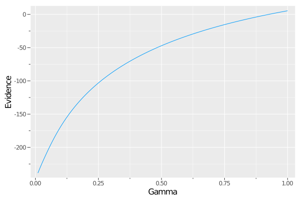
Consider . Furthermore, assume that for any . Then is a monotonically increasing function of .
Proof.
See Appendix A. ∎
Since the term is eliminated when considering the posterior distribution (2.1), this rescaling is a non-essential modification in the method we shall propose later. The meaning of the rescaling is to ensure that converges to the log-likelihood as , so that can be regarded as a natural extension of the log-likelihood.
The important point here is that Proposition 1 implies that there are theoretically at least some situations where evidence is increasing monotonically for . Indeed, the following numerical example vividly illustrates such a situation. To see this numerically, we consider a simple but motivating example in which and then randomly replace of by , where is called the contamination proportion. Here was determined by dividing equally into 1,000 points. In other words, in the context of Bayesian model selection, this corresponds to choosing the model with the largest evidence as to the best model out of 1,000 models indexed by . With the choice , we then calculated Monte Carlo estimates of the model evidence for each . The resulting are shown in Figure 2.1, which numerically shows that is a monotonically increasing function of so that it does not have local maxima. This implies that one cannot estimate using . A similar phenomenon is also discussed in Jewson and Rossell, 2021.
2.3 Estimation using H-score
To overcome the illustrated problem, we first treat as an unnormaliseable statistical model motivated by Hyvärinen, 2005. Note that even with an unnormalisable model, the update in (2.1) can be considered as a valid belief update according to Bissiri et al., 2016. It should be noted that when is the density power divergence of the form (2.2), the normalising constant may not exist. For example, when is a normal distribution, converges to a constant value under , so the integral of with respect to diverges. Recently, Jewson and Rossell, 2021 has pointed out that the role of such unnormalisable models can be recognised in terms of relative probability.
For dimensional observations and twice differentiable density , Hyvärinen, 2005 defines the H-score as
We then select the optimal with the smallest leave-one-out H-score, defined as
| (2.3) |
where and . Note that Shao et al., 2019 adoptes the H-score to define prequential score for state space models, and the criteria (2.3) can be seen as prequential score under i.i.d. settings. As shown in Appendix B, under the assumptions stated in Shao et al., 2019, the leave-one-out H-score (2.3) can be rewritten as
| (2.4) |
where the expectation is with respect to the robustified posterior distribution (2.1). Then, we can estimate as follows
| (2.5) |
As we shall discuss later, it can be shown that, under some conditions, converges to the Fisher divergence, Therefore, can be considered as an empirical approximation of the Fisher divergence for the marginal distribution based on unnormaliseable models defined by robust divergence. An important point here is that the estimation by the H-score is independent of the normalisation constant. The following proposition is theoretical justification of selecting via (2.5).
Proposition 2.
Let . Then, under the conditions stated in Appendix C, we have w.p.1. as .
Proof.
See Appendix C. ∎
Remark 1.
As we mentioned, the prequential version of is also called the H-score in the context of Bayesian model selection (Shao et al., 2019; Dawid et al., 2015). The main advantage of using the H-score in this context is that it will provide a consistent and coherent model selection criterion. Jewson and Rossell, 2021 proposes a consistent model selection criterion that is similarly based on H-scores but with batch estimation. Although the prequential method is coherent, this comes with a very high computational cost, for every model, one must do posterior inference on all permutations of the data and increasing sample sizes. Here, we use a batch estimation approach to estimate , which avoids high computational costs. We also want to emphasise that, as we shall study later, such a batch approach will give rise to natural and efficient algorithms to estimate and posterior sampling.
Under the density power divergence (2.2), the first and second order derivatives of are given by
These expressions do not include the integral term , which makes the calculation of much more straightforward in practice since the integral term often is a form of a complicated expression.
2.4 Numerical illustration of the H-score under normal distribution
We consider the same problem in the example in Subsection 2.2. For a normal distribution , the derivatives are as follows
where is the density function of . We calculated in (2.4) for each , where posterior expectations were approximated by posterior samples of . The data were simulated in the same way as in Subsection 2.2. The results are shown in Figure 2.2 when (blue lines) and (red lines). Our experiment shows numerically that has a local minimum. Furthermore, it can be seen that in regions where is small, the posterior mean is relatively heavily influenced by outliers. In contrast, the posterior mean settles to a constant value in regions where is greater than the value that minimises . Uncertainty in the sense of CI becomes greater. This result would suggest that statistical inefficiencies occur in regions where is larger than is necessary.

3 Sequential Monte Carlo Samplers
A natural way to obtain in (2.5) will be to use Robbins-Monro-type recursion.
| (3.1) |
where but, in general, posterior sampling based on the Monte Carlo approximation will be required to evaluate . That is, we need to construct an estimator of . To do so, we first treat in (3.1) as the positive sequence such that where is an artificial time index. Then (2.1) gives rise to the following tempering-like distributions on a common measurable space, say
| (3.2) |
The meaning of tempering-like here is not the usual tempering. It means that a family of distributions is constructed in the same measurable space by a sequence of updated , gradually approaching the target distribution in the sense of an optimised , say . Using this, we can define a sequence of distributions defined on product spaces
| (3.3) |
where is a transition kernel from to . Notice that admits marginally . Also let be a reversible MCMC kernel. Then it is given by
Since by construction, as the Radon–Nikodym derivative between them, one can derive unnormalised incremental weights as follows
| (3.4) |
For a detailed discussion of the choice of and and how the weights are derived, see e.g. Del Moral et al., 2006; Dai et al., 2020. Then the SMC samplers (Del Moral et al., 2006) iterate the following steps. First, the normalised weights are calculated for . Using these, one needs to sample ancestor indices from the categorical distribution induced by the normalised weights , denoted by . Finally, sample through for . We refer to Dai et al., 2020 for a number of recent advances in SMC samplers. As a result, we have the particle system that constructs an approximation of at any time step as required, where denotes the Dirac measure located at . Using the system, an approximation of can be obtained under appropriate regularity conditions that allow us to interchange differentiation with respect to and integration; see Appendix D for details. Therefore, an approximation of (3.1) will be
| (3.5) |
Given the time steps and initial , we update via (3.5) and iterate the SMC sampler times. Our method can be algorithmically summarised as follows.
- i)
Initialise the particles , with , , for .
- ii)
Apply the iteration
- iii)
Calculate in (3.4) and set for .
- iv)
Sample ancestor indices .
- v)
Sample particles for .
- vi)
Obtain estimate of .
Remark 2.
Since are independent of but dependent of , the particles can be sampled after resampling in 1. In addition, 1 uses a simple multinomial resampling applied at each step. The variability of the Monte Carlo estimates can be further reduced by incorporating dynamic resampling via the use of effective sample size. See Del Moral et al., 2006; Dai et al., 2020 for details.
Theoretical guarantees of convergence of the Robbins-Monro algorithm usually require that is unbiased. Even if is chosen adaptively, Beskos et al., 2016 shows that is still a (weakly) consistent estimator, but not an unbiased estimator. Such unbiased estimation may be possible by using the recently developed MCMC with couplings in 1, see Middleton et al., 2019; Jacob et al., 2020 for details. Instead of discussing convergence through such unbiased estimation, we shall discuss convergence through numerical experiments in the following sections.
We end this section by noting several advantages of the proposed method. First, 1 enables us to estimate the tuning parameter and obtain posterior sampling simultaneously. This is a notable difference from existing methods, such as running MCMC or the EM algorithm with a fixed tuning parameter, for example, Fujisawa and Eguchi, 2008; Ghosh and Basu, 2016. We believe that it may be emphasised that by setting up a well-defined target function and using the stochastic gradient framework-based SMC samplers, it is possible to avoid the two-stage estimation that many previous studies have done in this context. We also emphasise that our proposed method has two notable advantages over existing methods: it does not require pilot plots, and it does not require an expression of the asymptotic variance of the model. Next, recall that as , converges to Kullback–Leibler divergence. Let be the value of converged in 1. Then 1 may be producing an approximated bridge between (multiplied by a prior distribution) Kullback–Leibler divergence and the target distribution . Therefore, sampling from such tempering-like distributions induced by the density power divergence (3.2) could provide a beneficial tempering effect and a potential reduction in computational complexity, particularly when is large (Neal, 2001). Finally, 1 will give rise to a natural way to construct adaptive MCMC kernels. Suppose that we use Metropolis-Hastings kernels based on a Gaussian random walk. Notice that before MCMC step in 1, we have which approximates so that estimates , are available. Also Ghosh and Basu, 2016 shows that can be approximated by the Gaussian distribution. These will lead us to set , , for instance. We note that this proposal is also can be considered as a consequence of the results from the optimal scaling analysis for random walk Metoropolis, see Chopin, 2002; Chopin and Papaspiliopoulos, 2020 and references therein for more details.
4 Numerical Examples
To specify the schedule for the scaling parameters in (3.5), we use the standard adaptive method termed ADAM, by Kingma and Ba, 2014, known as stabilising the unnecessary numerical instability due to the choice of . Assume that after steps we have . ADAM applies the following iterative procedure,
where are the tuning parameters. The convergence properties of ADAM have been widely studied (Kingma and Ba, 2014; Reddi et al., 2019). Following closely Kingma and Ba, 2014, in all uses of ADAM below we set . ADAM is nowadays a standard and very effective addition to the type of recursive inference algorithms we are considering here, even more so as for increasing dimension of unknown parameters. See the above references for more motivation and details.
4.1 Simulation Studies
We here demonstrate the numerical performance of the proposed method. Throughout this study, we consider Gaussian models where both and are unknown parameters. We first simulated data and then randomly replaced of by . This setting is commonly referred to as the M-open world (Bernardo and Smith, 2009) in the sense that there is no such that .
Experiment 1: Convergence property
We investigate convergence behaviour of 1. In this study, we set with MCMC steps in 1 to estimate . The results are shown in Figure 4.1. As can be seen in the figure, our proposed method converges stably to the true value after about 100 iterations. Here, the true value was obtained by first approximating the H-score with MCMC in the same way as before and then using a grid search to find the that minimises it.


Experiment 2: Comparison with methods using fixed values of
We next compare the performance of our proposed method with that of a non-adaptive method using a fixed value of . We set , and for each case we computed the posterior distribution of using 1 and the vanilla version of MCMC. For 1, the tuning parameters were set to with MCMC steps, and for vanilla MCMC, was set to in advance of the estimation with 100,000 MCMC steps. We used Metropolis-Hastings kernels based on a Gaussian random walk with for the two cases under the uniform prior. Using the posterior samples obtained from 1 and non-adaptive methods, we computed the posterior mean and credible interval of . We ran 100 Monte Carlo experiments to calculate their (empirical) mean square error (MSE) and average 95 credible interval (ACI). The MSE is computed against the target value of 1, and the value is multiplied by 100. The results are given in Table 1. Although it is a simple example, the results summarised in the table clearly show that the accuracy of the inference is improved by estimating from the data rather than simply fixing it in terms of MSE. In fact, the best among the five choices depends on the underlying contamination ratio that we do not know in practice. Hence, it is difficult to determine a suitable value of simply by looking at the data, while our method can automatically tune the value of from the data. It should also be noted that the importance of adaptive tuning of is reflected in the results of not only MSE but also ACI; that is, the interval length obtained from 1 is narrow compared with the non-adaptive methods in all the four scenarios.
| MSE | 3.66 | 12.09 | 7.58 | 21.54 |
| ACI | (0.62, 1.06) | (1.08, 1.57) | (1.00, 1.49) | (1.18, 1.71) |
| MSE | 4.87 | 4.08 | 2.27 | 2.71 |
| ACI | (0.56, 1.10) | (0.82, 1.44) | (0.69, 1.28) | (0.65, 1.27) |
| () | ||||
| MSE | 6.27 | 4.79 | 3.32 | 4.86 |
| ACI | (0.49, 1.13) | (0.69, 1.45) | (0.61, 1.31) | (0.52, 1.24) |
| () | ||||
| MSE | 8.00 | 5.78 | 4.61 | 6.78 |
| ACI | (0.41, 1.18) | (0.58, 1.51) | (0.55, 1.38) | (0.43, 1.29) |
| () | ||||
| MSE | 10.04 | 8.35 | 6.44 | 8.90 |
| ACI | (0.33, 1.24) | (0.46, 1.59) | (0.47, 1.46) | (0.34, 1.35) |
| 0.006 | 0.207 | 0.213 | 0.272 | |
| MSE | 3.13 | 3.51 | 2.13 | 2.47 |
| ACI | (0.66, 1.05) | (0.91, 1.46) | (0.76, 1.32) | (0.67, 1.28) |
Experiment 3: Comparison with Jewson and Rossell, 2021
We next compare the proposed method with the H-posterior proposed by Jewson and Rossell, 2021 (denoted by JR hereafter), where the posterior of the model parameters as well as can be obtained. To apply the JR method, we generated 1000 posterior samples after discarding the first 500 samples. We evaluate the performance of the inference of and by MSE (multiplied by 100), coverage probability (CP) and average length (AL) of credible intervals. The results are shown in Table Table 2, where the average estimates of are also shown. Although both methods provide similar estimates of , the accuracy of point estimation of JR is slightly better than that of 1. However, it is observed that JR tends to produce a short coverage length so that the CP of the JR method is much smaller than the nominal level . Accordingly, the average length is much smaller than those by 1. This means that a direct application of the H-posterior by Jewson and Rossell, 2021 may fail to capture the uncertainty of the posterior compared with the proposed method.
| MSE | CP | AL | ||||||||
|---|---|---|---|---|---|---|---|---|---|---|
| mean | var | |||||||||
| 5 | 0.194 | 0.001 | 3.62 | 5.23 | 97 | 84 | 0.57 | 0.53 | ||
| 1 | 10 | 0.297 | 0.003 | 4.57 | 9.20 | 97 | 88 | 0.51 | 0.56 | |
| 15 | 0.377 | 0.009 | 1.06 | 12.60 | 92 | 82 | 0.61 | 0.67 | ||
| 5 | 0.193 | 0.011 | 2.33 | 5.10 | 68 | 13 | 0.27 | 0.16 | ||
| JR | 10 | 0.230 | 0.009 | 2.46 | 6.25 | 64 | 10 | 0.28 | 0.16 | |
| 15 | 0.261 | 0.013 | 2.50 | 7.27 | 68 | 5 | 0.29 | 0.15 | ||
Experiment 4: Comparison with tempering
Following Nakagawa and Hashimoto, 2020, we compare the robustness to outliers for the two generalised posterior distributions. The first distribution is constructed in the same way as before, while the other is constructed using tempering. We specify a tempered posterior as where . To construct the sequence, we divided the interval into 500 equal parts. We applied 1 and the SMC sampler with the tempered posterior to test the robustness of the proposed method to data sets containing outliers. We used particles, MCMC steps for both methods, and set for 1. The prior and MCMC kernels were set as the previous experiment, and the density estimation results obtained from the estimation results are summarised in Figure 4.2. The red line represents the posterior density estimate for when the data do not contain any outliers, and the blue line represents it when the data contain outliers. It is clear from the estimation results that our proposed method is robust even when the dataset contains outliers, while the SMC sampler with the tempered posterior is greatly affected by outliers, and the estimated posterior distributions are completely separated as a result.

4.2 Applications to Real Data
Newcomb data
We apply our methodology to Simon Newcomb’s measurements of the speed of light data, motivated by applications in Stigler, 1977; Basu et al., 1998; Basak et al., 2021. The data can be obtained from Andrew Gelman’s webpage: http://www.stat.columbia.edu/~gelman/book/data/light.asc. The sample size of the data set is 66 and contains two outliers, -44 and -2, illustrated in Figure 4.3. We fitted a Gaussian distribution model to the data and used 1 to obtain the posterior distribution of the parameters . The tuning parameters in 1 were set to with MCMC iterations. The MCMC kernel was constructed as in the previous examples, and results are given in Figure 4.4. The existing study (Basak et al., 2021) reported for the same data set, which is very high compared to our estimate result of . Since the method proposed in Basak et al., 2021 requires a pilot plot and the estimation results depend significantly on it, we believe our estimation results are more reasonable. In fact, it is unlikely that we will have to use a value of for a data set that contains only two outliers. As shown in Basu et al., 1998, the parameter estimates are almost the same when and when . However, from the point of view of statistical efficiency, it would be preferable to adopt the lower value of if the estimates were the same. To confirm this, bootstrap resamplings were performed on the data, and the posterior bootstrap mean of each parameter and the variance was calculated, reported in Table 3. For each re-sampled data, we compared the results when the posterior distribution was calculated while estimating with our method and when the posterior distribution was calculated using MCMC after estimating and fixing it with the method proposed in Basak et al., 2021. The numerical experiments show that although the means estimated parameters agree between the two methods, the variances are much smaller for our method, suggesting that overestimation of leads to statistical inefficiency.


| mean() | var() | mean() | var() | |
|---|---|---|---|---|
| 1 | 27.559 | 0.0017 | 5.7605 | 0.0013 |
| Basak et al., 2021 | 27.674 | 0.4351 | 5.3976 | 0.5295 |
Hertzsprung–Russell Star Cluster Data
We use our methodology to perform linear regression models with normal errors, that is . Motivated by Basak et al., 2021, we fitted the regression model to the Hertzsprung-Russell star cluster data (Rousseeuw and Leroy, 2005), without constants. The data set contains 47 observations on the logarithm of the effective temperature at the surface of the CYG OB1 star cluster (Te, covariates ) and the logarithm of its light intensity (L/L0, explained variables ). The data can be obtained from https://rdrr.io/cran/robustbase/man/starsCYG.html, and shown at Figure 4.5. The tuning parameters in 1 were set to with MCMC iterations, and we used the uniform prior for . The MCMC kernel was constructed as in the previous examples, and results are given in Figure 4.6. The corresponding OLS estimates were . Whilst we obtained , Basak et al., 2021 reported for the same data set. Our numerical experiments and previous studies (Ghosh and Basu, 2016; Nakagawa and Hashimoto, 2020) will suggest that as the proportion of outliers in the data increases, the value of also tends to increase. Thus, such a large value of is not reasonable considering the proportion of outliers in the data (only four samples in the lower right part in Figure 4.5), suggesting the superiority of our proposed method. Indeed, to confirm the suggested statistical inefficiency, the same experiments as in the previous section were carried out, and the results are summarised in Table 4. Although the results are not as striking as in the previous Newcomb data example, it would be possible to confirm that statistical inefficiencies occur in the estimation by the proposed method in Basak et al., 2021 in the regression model as well.


| mean() | var() | mean() | var() | |
|---|---|---|---|---|
| 1 | 0.8514 | 0.0002 | 0.6100 | 0.0037 |
| Basak et al., 2021 | 0.8763 | 0.0299 | 0.6536 | 0.0708 |
5 Concluding remarks
Our proposed method performs reasonably well and provides one of the few options, as far as we know, for routine robust Bayesian inference. To the best of our knowledge, this is the first attempt to propose both a theory and a computational algorithm to estimate the tuning parameters from data and to allow robust Bayesian estimation. We have shown numerically that a more efficient Bayesian estimation can be achieved by estimating the tuning parameter from the data. We have proposed an efficient sampling method using SMC samplers considering the sequence of as the temperature. Compared to existing studies (Warwick and Jones, 2005; Basak et al., 2021), our method has specificity and usefulness in that we can estimate the tuning parameters and sample from the posterior distribution simultaneously, and pilot plots and the asymptotic variance formula are not necessary. In this paper, we have focused in particular on the case of the density power divergence, but we want to stress that our method is general enough in the sense that it can be applied to the Bayesian estimation of other robust divergence-induced models.
Furthermore, our framework opens up a number of routes for future research and insight, including those described below.
- i)
As we have noted, the integral term is eliminated in the H-score, while the computation of the posterior distribution is computationally expensive, so it may be better to consider the H-posterior studied in Jewson and Rossell, 2021 in this respect. However, the robustness of the H-posterior has not yet been studied, and it would therefore be interesting in the future to investigate this point in more detail using the influence function.
- ii)
Another direction of investigation involves the construction of an efficient MCMC kernel for posterior distributions derived from robust divergence such as (2.1). To make good inferences from data containing outliers, the posterior distribution induced by robust divergence is a model with a more or less heavy-tailed. As studied in Kamatani, 2018, many standard MCMC algorithms are known to perform poorly in such cases, especially in higher dimensions. Therefore, studying MCMC algorithms within 1 tailored to the posterior distribution induced by robust divergence would allow for more efficient Bayesian robust estimation.
- iii)
In this study, we have not focused on time series data, but, as Shao et al., 2019 shows, the H-score can also be defined for models that are not independent, for example, state-space models. In fact, Boustati et al., 2020 proposes a method for Bayesian filtering of state-space models using robust divergence, but the tuning parameters need to be estimated before filtering, and in this sense, it is not online filtering. 1 does batch estimation, but we believe that extending it to online estimation would allow robust filtering of the state-space model while estimating the tuning parameters online from the data.
- iv)
This study has focused on estimation and computational methods proposed in the generalised Bayesian framework, particularly using robust divergence. On the other hand, methods using the Maximum Mean Discrepancy (Chérief-Abdellatif and Alquier, 2020) and Kernel Stein Discrepancy (Matsubara et al., 2022) have also been proposed in recent years in the same generalised Bayesian framework, although not with the motivation of dealing with outliers. Both require adjustment of the hyperparameters of the kernel used, and it may be possible to estimate them using our proposed method and compare their performance. We have avoided comparing these potential alternative approaches because we believe this would obscure the main messages we have tried to convey within the numerical results section. Such a detailed numerical study can be the subject of future work.
Acknowledgement
SY was supported by the Japan Society for the Promotion of Science (KAKENHI) under grant number 21K17713. SS was supported by the Japan Society for the Promotion of Science (KAKENHI) under grant number 21H00699.
References
- Azlarov and Volodin, (1982) Azlarov, T. A. and Volodin, N. A. (1982). Laws of large numbers for identically distributed banach-space valued random variables. Theory of Probability & Its Applications, 26(3):573–580.
- Basak et al., (2021) Basak, S., Basu, A., and Jones, M. (2021). On the optimal density power divergence tuning parameter. Journal of Applied Statistics, 48(3):536–556.
- Basu et al., (1998) Basu, A., Harris, I. R., Hjort, N. L., and Jones, M. (1998). Robust and efficient estimation by minimising a density power divergence. Biometrika, 85(3):549–559.
- Bernardo and Smith, (2009) Bernardo, J. M. and Smith, A. F. (2009). Bayesian theory, volume 405. John Wiley & Sons.
- Beskos et al., (2016) Beskos, A., Jasra, A., Kantas, N., and Thiery, A. (2016). On the convergence of adaptive sequential monte carlo methods. The Annals of Applied Probability, 26(2):1111–1146.
- Beskos et al., (2009) Beskos, A., Papaspiliopoulos, O., and Roberts, G. (2009). Monte carlo maximum likelihood estimation for discretely observed diffusion processes. The Annals of Statistics, 37(1):223–245.
- Bissiri et al., (2016) Bissiri, P. G., Holmes, C. C., and Walker, S. G. (2016). A general framework for updating belief distributions. Journal of the Royal Statistical Society. Series B, Statistical methodology, 78(5):1103.
- Boustati et al., (2020) Boustati, A., Akyildiz, Ö. D., Damoulas, T., and Johansen, A. (2020). Generalized bayesian filtering via sequential monte carlo. arXiv preprint arXiv:2002.09998.
- Chérief-Abdellatif and Alquier, (2020) Chérief-Abdellatif, B.-E. and Alquier, P. (2020). Mmd-bayes: Robust bayesian estimation via maximum mean discrepancy. In Symposium on Advances in Approximate Bayesian Inference, pages 1–21. PMLR.
- Chopin, (2002) Chopin, N. (2002). A sequential particle filter method for static models. Biometrika, 89(3):539–552.
- Chopin and Papaspiliopoulos, (2020) Chopin, N. and Papaspiliopoulos, O. (2020). An introduction to sequential Monte Carlo. Springer.
- Cichocki and Amari, (2010) Cichocki, A. and Amari, S.-i. (2010). Families of alpha-beta-and gamma-divergences: Flexible and robust measures of similarities. Entropy, 12(6):1532–1568.
- Cichocki et al., (2011) Cichocki, A., Cruces, S., and Amari, S. (2011). Generalized alpha-beta divergences and their application to robust nonnegative matrix factorization. Entropy, 13(1):134–170.
- Dai et al., (2020) Dai, C., Heng, J., Jacob, P. E., and Whiteley, N. (2020). An invitation to sequential monte carlo samplers.
- Dawid et al., (2015) Dawid, A. P., Musio, M., et al. (2015). Bayesian model selection based on proper scoring rules. Bayesian analysis, 10(2):479–499.
- Del Moral et al., (2006) Del Moral, P., Doucet, A., and Jasra, A. (2006). Sequential monte carlo samplers. Journal of the Royal Statistical Society: Series B (Statistical Methodology), 68(3):411–436.
- Fong and Holmes, (2020) Fong, E. and Holmes, C. (2020). On the marginal likelihood and cross-validation. Biometrika, 107(2):489–496.
- Frazier et al., (2021) Frazier, D. T., Loaiza-Maya, R., Martin, G. M., and Koo, B. (2021). Loss-based variational bayes prediction. arXiv preprint arXiv:2104.14054.
- Fujisawa and Eguchi, (2008) Fujisawa, H. and Eguchi, S. (2008). Robust parameter estimation with a small bias against heavy contamination. Journal of Multivariate Analysis, 99(9):2053–2081.
- Ghosh and Basu, (2016) Ghosh, A. and Basu, A. (2016). Robust bayes estimation using the density power divergence. Annals of the Institute of Statistical Mathematics, 68(2):413–437.
- Ghosh et al., (2017) Ghosh, A., Harris, I. R., Maji, A., Basu, A., Pardo, L., et al. (2017). A generalized divergence for statistical inference. Bernoulli, 23(4A):2746–2783.
- Hashimoto and Sugasawa, (2020) Hashimoto, S. and Sugasawa, S. (2020). Robust bayesian regression with synthetic posterior distributions. Entropy, 22(6):661.
- Hyvärinen, (2005) Hyvärinen, A. (2005). Estimation of non-normalized statistical models by score matching. Journal of Machine Learning Research, 6(4).
- Jacob et al., (2020) Jacob, P. E., O’Leary, J., and Atchadé, Y. F. (2020). Unbiased markov chain monte carlo methods with couplings. Journal of the Royal Statistical Society: Series B (Statistical Methodology), 82(3):543–600.
- Jewson and Rossell, (2021) Jewson, J. and Rossell, D. (2021). General bayesian loss function selection and the use of improper models. arXiv preprint arXiv:2106.01214.
- Jewson et al., (2018) Jewson, J., Smith, J. Q., and Holmes, C. (2018). Principles of bayesian inference using general divergence criteria. Entropy, 20(6):442.
- Kamatani, (2018) Kamatani, K. (2018). Efficient strategy for the markov chain monte carlo in high-dimension with heavy-tailed target probability distribution. Bernoulli, 24(4B):3711–3750.
- Kingma and Ba, (2014) Kingma, D. P. and Ba, J. (2014). Adam: A method for stochastic optimization. arXiv preprint arXiv:1412.6980.
- Knoblauch et al., (2018) Knoblauch, J., Jewson, J., and Damoulas, T. (2018). Doubly robust bayesian inference for non-stationary streaming data with -divergences. arXiv preprint arXiv:1806.02261.
- Knoblauch et al., (2019) Knoblauch, J., Jewson, J., and Damoulas, T. (2019). Generalized variational inference: Three arguments for deriving new posteriors. arXiv preprint arXiv:1904.02063.
- Matsubara et al., (2022) Matsubara, T., Knoblauch, J., Briol, F.-X., Oates, C., et al. (2022). Robust generalised bayesian inference for intractable likelihoods. Journal of the Royal Statistical Society: Series B.
- Middleton et al., (2019) Middleton, L., Deligiannidis, G., Doucet, A., and Jacob, P. E. (2019). Unbiased smoothing using particle independent metropolis-hastings. In The 22nd International Conference on Artificial Intelligence and Statistics, pages 2378–2387. PMLR.
- Nakagawa and Hashimoto, (2020) Nakagawa, T. and Hashimoto, S. (2020). Robust bayesian inference via -divergence. Communications in Statistics-Theory and Methods, 49(2):343–360.
- Neal, (2001) Neal, R. M. (2001). Annealed importance sampling. Statistics and computing, 11(2):125–139.
- Nielsen et al., (2017) Nielsen, F., Sun, K., and Marchand-Maillet, S. (2017). On hölder projective divergences. Entropy, 19(3):122.
- Reddi et al., (2019) Reddi, S. J., Kale, S., and Kumar, S. (2019). On the convergence of adam and beyond. arXiv preprint arXiv:1904.09237.
- Rousseeuw and Leroy, (2005) Rousseeuw, P. J. and Leroy, A. M. (2005). Robust regression and outlier detection, volume 589. John wiley & sons.
- Shao et al., (2019) Shao, S., Jacob, P. E., Ding, J., and Tarokh, V. (2019). Bayesian model comparison with the hyvärinen score: Computation and consistency. Journal of the American Statistical Association.
- Stigler, (1977) Stigler, S. M. (1977). Do robust estimators work with real data? The Annals of Statistics, pages 1055–1098.
- Warwick and Jones, (2005) Warwick, J. and Jones, M. (2005). Choosing a robustness tuning parameter. Journal of Statistical Computation and Simulation, 75(7):581–588.
Appendix A Proof of Proposition 1
Recall that . First, is an increasing function of for arbitrary and . Furthermore, since we have assumed that , it holds that for and arbitrary , so that is a decreasing function of . Hence, is increasing since it is a sum of two increasing functions.
Appendix B Derivation of (2.4)
For simplicity, we consider , but the extension to the general dimension is straightforward. Let be a general model with parameter and be the marginal likelihood under prior . Under the assumptions stated in supplement (S6) in Shao et al., 2019, the following identify always holds
where the expectation is taken with respect to the posterior distribution of given . Using the above identity with , and , where , we have
Notice that, since we have assumed observations, we have . Hence, the expression (2.4) follows by setting .
Appendix C Proof of Proposition 2
The proof here is essentially the same as Shao et al., 2019 and Jewson and Rossell, 2021, so we only provide an overview of the proof. Assume that, for simplicity, . First one can show that can be decomposed into the sum of conditional expectation terms of , and the sum of conditional variance terms of , see Dawid et al., 2015; Shao et al., 2019. Then under the assumptions stated in supplement of Shao et al., 2019, the variance term will converge at w.p.1. Let be the space of continuous real functions on the compact set of equipped with the sup-norm. Then, under the same assumptions, may take values in this space. Then strong law of large numbers on a separable Banach space (Azlarov and Volodin, 1982; Beskos et al., 2009), may be applied to . Combining this result with (s10) in supplement of Shao et al., 2019 and integration by parts (Hyvärinen, 2005; Dawid et al., 2015) would yield w.p.1. The result follows under the assumption for identification such that is only maximised at , see A1. in Jewson and Rossell, 2021 for instance.
Appendix D Derivatives of the H-score
In the following argument, we assume the exchangeability of integral and derivative without any remarks. For simplicity, we consider a univariate case, namely . We define and . The derivative of the H-score with respect to is expressed as
which requires the computation of integral of the following form:
| (D.1) |
where
| (D.2) |
and . It follows that
where the third term is further simplified to
Hence, the derivative (D.1) is expressed as
| (D.3) |
Finally, the derivative of the H-score is expressed as
| (D.4) |
where and are defined in (D.2).
D.1 General case
Let be a parametric density of . The density power divergence (Basu et al., 1998) is
noting that the second term is irrelevant in the computation of the H-score since it does not depend on . The detailed expressions of the quantities that appear in the derivative of the H-score in (D.4) are obtained as follows:
D.2 Normal distribution case
When , the corresponding density power divergence is
The detailed expressions of quantities appeared in the derivative of the H-score in (D.4) are obtained as follows:
where . When , the derivative of the H score in the model is obtained by replacing with .