Stochastic Alternating Direction Method of Multipliers
for Byzantine-Robust Distributed Learning

Most of the traditional machine learning algorithms require to collect training data from their owners to a single computer or data center, which is not only communication-inefficient but also vulnerable to privacy leakage [1, 2, 3]. With the explosive growth of the big data, federated learning has been proposed as a novel privacy-preserving distributed machine learning scheme, and received extensive research interest recently [4, 5, 6]. In federated learning, the training data are stored at distributed workers, and the workers compute their local variables using local training data, under the coordination of a master. This scheme effectively reduces the risk of data leakage and protects privacy.

However, federated learning still faces significant security challenges. Some of the distributed workers, whose identities are unknown, could be unreliable and send wrong or even malicious messages to the master, due to data corruptions, computation errors or malicious attacks. To characterize the worse-case scenario, we adopt the Byzantine failure model, in which the Byzantine workers are aware of all information of the other workers, and able to send arbitrary messages to the master [7, 8, 9, 10]. In this paper, we aim at solving the distributed learning problem under Byzantine attacks that potentially threat federated learning applications.

Related works. With the rapid popularization of federated learning, Byzantine-robust distributed learning has become an attractive research topic in recent years. Most of the existing algorithms modify distributed stochastic gradient descent (SGD) to the Byzantine-robust variants. In the standard distributed SGD, at every iteration, all the workers send their local stochastic gradients to the master, while the master averages all the received stochastic gradients and updates the optimization variable. When Byzantine workers are present, they can send faulty values other than true stochastic gradients to the master so as to bias the learning process. It is shown that the standard distributed SGD with mean aggregation is vulnerable to Byzantine attacks [11].

When the training data are independently and identically distributed (i.i.d.) at the workers, the stochastic gradients of the regular workers are i.i.d. too. This fact motivates two mainstream methods to deal with Byzantine attacks: attack detection and robust aggregation. For attack detection, [12] and [13] propose to offline train an autoencoder, which is used to online calculate credit scores of the workers. The messages sent by the workers with lower credit scores will be discarded in the mean aggregation. The robust subgradient push algorithm in [14] operates over a decentralized network. Each worker calculates a score for each of its neighbors, and isolates those with lower scores. The works of [15, 16] detect the Byzantine workers with historic gradients so as to ensure robustness. The work of [17] uses redundant gradients for attack detection. However, it requires overlapped data samples on multiple workers, and does not fit for the federated learning setting. For robust aggregation, the master can use geometric median, instead of mean, to aggregate the received messages [18, 19, 20]. When the number of Byzantine workers is less than the number of regular workers, geometric median provides a reliable approximation to the average of regular workers’ stochastic gradients. Other similar robust aggregation rules include marginal trimmed mean and dimensional median [21, 22, 23]. Some aggregation rules select a representative stochastic gradient from all the received ones to update the global variable, e.g., Medoid [19] and Krum [11]. Medoid selects the stochastic gradient with the smallest distance from all the others, while Krum selects the one with the smallest squared distance to a fixed number of nearest stochastic gradients. An extension of Krum, termed as $h$-Krum, selects $h$ stochastic gradients with Krum and uses their average. Bulyan [24] first selects a number of stochastic gradients with Krum or other robust selection/aggregation rules, and then uses their trimmed dimensional median.

When the training data and the stochastic gradients are non-i.i.d. at the workers, which is common in federated learning applications [25], naive robust aggregation of stochastic gradients no longer works. The works of [26, 27] adopt a resampling strategy to alleviate the effect caused by non-i.i.d. training data. With a larger resampling parameter, the algorithms can handle higher data heterogeneity, at the cost of tolerating less Byzantine workers. Robust stochastic aggregation (RSA) aggregates local variables, instead of stochastic gradients [28]. To be specific, it considers a total variation (TV) norm-penalized approximation formulation to handle Byzantine attacks, where the TV norm penalty forces the regular workers’ local variables to be close, and meanwhile, tolerates the outliers sent by the Byzantine workers. Although the stochastic subgradient method proposed in [28] is able to solve the TV norm-penalized approximation formulation, it ignores the separable problem structure.

Other related works include [29, 30, 31, 32], which shows that the stochastic gradient noise affects the effectiveness of robust aggregation rules. Thus, the robustness of the Byzantine-resilience methods can be improved by reducing the variance of stochastic gradients. The asynchronous Byzantine-robust SGD is considered in [33, 34, 35]. The work of [36] addresses the saddle-point attacks in the non-convex setting, and [37, 38, 39, 40] consider Byzantine robustness in decentralized learning.

Our contributions. Our contributions are three-fold.

(i) We propose a Byzantine-robust stochastic alternating direction method of multipliers (ADMM) that utilizes the separable problem structure of the TV norm-penalized approximation formulation. The stochastic ADMM updates are further simplified, such that the iteration-wise communication and computation costs are the same as those of the stochastic subgradient method.

(ii) We theoretically prove that the proposed stochastic ADMM converges to a bounded neighborhood of the optimal solution at a rate of $O(1/k)$ under mild assumptions, where $k$ is the number of iterations and the size of neighborhood is determined by the number of Byzantine workers.

(iii) We conduct numerical experiments on the MNIST and COVERTYPE datasets to demonstrate the effectiveness of the proposed stochastic ADMM to various Byzantine attacks.

Let us consider a distributed network with a master and $m$ workers, among which $q$ workers are Byzantine and the other $r=m-q$ workers are regular. The exact value of $q$ and the identities of the Byzantine workers are all unknown. We are interested in solving a stochastic optimization problem in the form of

where $\tilde{x}\in\mathbb{R}^{d}$ is the optimization variable, $f_{0}(\tilde{x})$ is the regularization term known to the master, and $F(\tilde{x},\xi_{i})$ is the loss function of worker $i$ with respect to a random variable $\xi_{i}\sim\mathcal{D}_{i}$. Here we assume that the data distributions $\mathcal{D}_{i}$ on the workers can be different, which is common in federated learning applications.

Define $\mathcal{R}$ and $\mathcal{B}$ as the sets of regular workers and Byzantine workers, respectively. We have $|\mathcal{B}|=q$ and $|\mathcal{R}|=r$. Because of the existence of Byzantine workers, directly solving (1) without distinguishing between regular and Byzantine workers is meaningless. A less ambitious alternative is to minimize the summation of the regular workers’ local expected cost functions plus the regularization term, in the form of

Our proposed algorithm and RSA [28] both aggregate optimization variables, instead of stochastic gradients. To do so, denote $x_{i}$ as the local copy of $\tilde{x}$ at a regular worker $i\in\mathcal{R}$, and $x_{0}$ as the local copy at the master. Collecting the local copies in a vector $x=[x_{0};\cdots;x_{i};\cdots]\in\mathbb{R}^{(r+1)d}$, we know that (2) is equivalent to

where $x_{i}-x_{0}=0$, $\forall i\in\mathcal{R}$ are the consensus constraints to force the local copies to be the same.

RSA [28] considers a TV norm-penalized approximation formulation of (3), in the form of

where $\lambda$ is a positive constant and $\sum_{i\in\mathcal{R}}\|x_{i}-x_{0}\|_{1}$ is the TV norm penalty for the constraints in (3). The TV norm penalty forces the regular workers’ local optimization variables to be close to the master’s, and meanwhile, tolerates the outliers when the Byzantine attackers are present. Due to the existence of the nonsmooth TV norm term, RSA solves (4) with the stochastic subgradient method. The updates of RSA, at the existence of Byzantine workers, are as follows. At time $k$, the master sends $x_{0}^{k}$ to the workers, every regular worker $i\in\mathcal{R}$ sends $x_{i}^{k}$ to the master, while every Byzantine worker $j\in\mathcal{B}$ sends an arbitrary malicious vector $u_{j}^{k}\in\mathbb{R}^{d}$ to the master. Then, the updates of $x^{k+1}_{i}$ for every regular worker $i$ and $x^{k+1}_{0}$ for the master are given by

where $F^{\prime}(x_{i}^{k},\xi^{k}_{i})$ is a stochastic gradient at $x_{i}^{k}$ respect to a random sample $\xi_{i}^{k}$ for regular worker $i$, $sgn(\cdot)$ is the element-wise sign function ($sgn(a)=1$ if $a>0$, $sgn(a)=-1$ if $a<0$, and $sgn(a)\in[-1,1]$ if $a=0$), and $\alpha^{k}$ is the diminishing learning rate at time $k$.

Although RSA has been proven as a robust algorithm under Byzantine attacks [28], the sign functions therein enable the Byzantine workers to send slightly modified messages that remarkably biases the learning process. In addition, RSA fully ignores the special separable structure of the TV norm penalty. In this paper, we also consider the TV norm-penalized approximation formulation (4), propose a stochastic ADMM that utilizes the problem structure, and develop a novel Byzantine-robust algorithm.

In this section, we utilize the separable problem structure of (4) and propose a robust stochastic ADMM to solve it. The challenge is that the unknown Byzantine workers can send faulty messages during the optimization process. At this stage, we simply ignore the existence of Byzantine workers and develop an algorithm to solve (4). Then, we will consider the influence of Byzantine workers on the algorithm. We begin with applying the stochastic ADMM to solve (4), and then simplify the updates such that the iteration-wise communication and computation costs are the same as those of the stochastic subgradient method in [28].

Stochastic ADMM. Suppose that all the workers are regular such that $m=r$. To apply the stochastic ADMM, for every worker $i$, introduce auxiliary variables $z(0,i),z(i,0)\in\mathbb{R}^{d}$ on the directed edges $(0,i),(i,0)$, respectively. By introducing consensus constraints $z(i,0)=x_{0}$ and $z(0,i)=x_{i}$, (4) is equivalent to

For the ease of presentation, we stack these auxiliary variables in a new variable $z\in\mathbb{R}^{2rd}$. As we will see below, the introduction of $z$ is to split the expectation term $\sum_{i\in\mathcal{R}}\mathbb{E}[F(x_{i},\xi_{i})]$ and the TV norm penalty term $\sum_{i\in\mathcal{R}}\|x_{i}-x_{0}\|_{1}$ so as to utilize the separable problem structure.

The augmented Lagrangian function of (6) is

where $\beta$ is a positive constant, while $\eta(i,0)\in\mathbb{R}^{d}$ and $\eta(0,i)\in\mathbb{R}^{d}$ are the Lagrange multipliers attached to the consensus constraints $z(i,0)-x_{0}=0$ and $z(0,i)-x_{i}=0$, respectively. For convenience, we also collect all the Lagrange multipliers in a new variable $\eta\in\mathbb{R}^{2rd}$.

Given the augmented Lagrangian function (3), the vanilla ADMM works as follows. At time $k$, it first updates $x^{k+1}$ through minimizing the augmented Lagrangian function at $z=z^{k}$ and $\eta=\eta^{k}$, then updates $z^{k+1}$ through minimizing the Lagrangian function at $x=x^{k+1}$ and $\eta=\eta^{k}$, and finally updates $\eta^{k+1}$ through dual gradient ascent. The updates are given by

However, the $x$-update in (8a) is an expectation minimization problem and hence nontrivial. To address this issue, [41] proposes to replace the augmented Lagrangian function $\mathcal{L}_{\beta}(x,z^{k},\eta^{k})$ with its stochastic counterpart, given by

where $\xi_{i}^{k}$ is the random variable of worker $i$ at time $k$ and $\sigma^{k}$ is the positive stepsize. Observe that (3) is a stochastic first-order approximation to (3), in the sense that

at the points $x_{i}=x_{i}^{k}$ and $x_{0}=x_{0}^{k}$, respectively.

With the stochastic approximation, the explicit solutions of $x_{i}^{k+1}$ and $x_{0}^{k+1}$ are

For simplicity, we replace the parameter $\frac{1}{\sigma^{k}+\beta}$ by $\alpha_{i}^{k}$ and $\frac{1}{\sigma^{k}+\sum_{i\in\mathcal{R}}\beta}$ by $\alpha_{0}^{k}$. Thus, (10) is equivalent to

Simplification. Observe that the $z$-update in (8b) is also challenging as the variables $z(0,i)$ and $z(i,0)$ are coupled by the TV norm penalty term. Next, we will simplify the three-variable updates in (11), (8b) and (8c) to eliminate the $z$-update and obtain a more compact algorithm. Note that the decentralized deterministic ADMM can also be simplified to eliminate auxiliary variables [42]. However, we are considering the distributed stochastic ADMM, and the TV norm penalty term makes the simplification much more challenging.

Presence of Byzantine workers. Now we start to consider how the stochastic ADMM updates (12), (13) and (14) are implemented when the Byzantine workers are present. At time $k$, every regular worker $i\in\mathcal{R}$ updates $x_{i}^{k+1}$ with (12) and $\eta^{k+1}_{i}$ with (14), and then sends $\eta_{i}^{k+1}$ to the master. Meanwhile, every Byzantine worker $j\in\mathcal{B}$ can cheat the master by sending $\eta_{j}^{k+1}\mathbb{R}^{d}$ where the elements are arbitrary within $[-\lambda,\lambda]^{d}$. Otherwise, the Byzantine worker $j$ can be directly detected and eliminated by the master. This amounts to that every Byzantine worker $j\in\mathcal{B}$ follows an update rule similar to (14), as

where $u^{k+1}_{j}\in\mathbb{R}^{d}$ is an arbitrary vector. After receiving all messages $\eta_{i}^{k+1}$ from the regular workers $i\in\mathcal{R}$ and $\eta_{j}^{k+1}$ from the Byzantine workers $j\in\mathcal{B}$, the master updates $x_{0}^{k+1}$ via

The Byzantine-robust stochastic ADMM for distributed learning is outlined in Algorithm 1 and illustrated in Figure 1. Observe that the communication and computation costs are the same as those in the stochastic subgradient method in [28]. The only extra cost is that every worker $i$ must store the dual variable $\eta^{k}_{i}$.

Comparing the stochastic subgradient updates (5) with the stochastic ADMM updates (12), (13) and (14), we can observe a primal-dual connection. In the stochastic subgradient method, the workers upload primal variables $x_{i}^{k}$, while in the stochastic ADMM, the workers upload dual variables $\eta_{i}^{k+1}$. The stochastic subgradient method controls the influence of a malicious message by the sign function. No matter what the malicious message is, its modification on each dimension is among $-\lambda$, $\lambda$, and a value within $[-\lambda,\lambda]$ if the values of the malicious worker and the master are identical. The stochastic ADMM controls the influence of a malicious message by the projection function. The modification of the malicious message on each dimension is within $[-\lambda,\lambda]$.

In this section, we analyze the convergence of the proposed Byzantine-robust stochastic ADMM. We make the following assumptions, which are common in analyzing distributed stochastic optimization algorithms.

In this section, we evaluate the robustness of the proposed algorithm to various Byzantine attacks. We compare the proposed Byzantine-robust Stochastic ADMM with the following benchmark algorithms: (i) Ideal SGD without Byzantine attacks; (ii) SGD subject to Byzantine attacks; (iii) Geometric median stochastic gradient aggregation [18, 19]; (iv) Median stochastic gradient aggregation [18, 19]; (v) RSA [28]. All the parameters of the benchmark algorithms are hand-tuned to the best. Although the stochastic ADMM and RSA are rooted in the same problem formulation (4), they perform differently for the same value of $\lambda$ due to Byzantine attacks, as we have observed in Example 1. Therefore, we hand-tune the best $\lambda$ for the stochastic ADMM and RSA, respectively. In the numerical experiments, we use two datasets, MNIST¹¹ 1 http://yann.lecun.com/exdb/mnist and COVERTYPE²² 2 https://www.csie.ntu.edu.tw/~cjlin/libsvmtools/datasets. The statistics of these datasets are shown in Table 1. We launch one master and 20 workers. In the i.i.d case, we conduct experiments on both datasets by randomly and evenly splitting the data samples to the workers, while in the non-i.i.d. case we only use the MNIST dataset. Each regular worker uses a mini-batch of 32 samples to estimate the local gradient at each iteration. The loss functions $f_{i}(\tilde{x})$ of workers are softmax regressions, and the regularization term is given by $f_{0}(\tilde{x})=\frac{0.01}{2}\|\tilde{x}\|^{2}$. Performance is evaluated by the top-1 accuracy.

Gaussian attack. Under Gaussian attack, at every iteration every Byzantine worker sends to the master a random vector, whose elements follow the Gaussian distribution with standard deviation $100$. Here we set the number of Byzantine workers $q=8$. For Stochastic ADMM on the MNIST dataset, we set $\lambda$ = 0.5, $\beta=0.5$, $\alpha_{0}^{k}=\frac{1}{10+10\sqrt{k}}$, and $\alpha_{i}^{k}=\frac{1}{0.5+10\sqrt{k}}$. As shown in Figure 3(a), SGD fails, Stochastic ADMM, RSA and Geometric median perform very similarly and are close to Ideal SGD, while Median is a little worse than the others. On the COVERTYPE dataset, we set $\lambda$ = 0.5, $\beta=0.1$, $\alpha_{0}^{k}=\frac{1}{2+50\sqrt{k}}$, and $\alpha_{i}^{k}=\frac{1}{0.1+50\sqrt{k}}$ for Stochastic ADMM. As shown in Figure 3(b), SGD performs the worst, while Stochastic ADMM, Geometric median, and median are close to Ideal SGD. Among all the Byzantine-robust algorithms, Stochastic ADMM has the fastest converge speed.

Sign-flipping attack. Under sign-flipping attack, at every iteration every Byzantine worker calculates its local variable, but flips the sign by multiplying with a constant $\varepsilon<0$, and sends to the master. Here we set $\varepsilon=-3$ and the number of Byzantine workers $q=8$. On the MNIST dataset, we set the parameters of Stochastic ADMM as $\lambda=0.05$, $\beta=0.1$, $\alpha_{0}^{k}=\frac{1}{2+5\sqrt{k}}$, and $\alpha_{i}^{k}=\frac{1}{0.1+5\sqrt{k}}$. Figure 4(a) shows that SGD also fails in this situation. Stochastic ADMM, RSA, and Geometric median are close to Ideal SGD, and achieve better accuracy than median. In Figure 4(b), shows the performance on the COVERTYPE dataset. The parameters of Stochastic ADMM are $\lambda=0.5$, $\beta=0.3$, $\alpha_{0}^{k}=\frac{1}{6+100\sqrt{k}}$ ,and $\alpha_{i}^{k}=\frac{1}{0.3+100\sqrt{k}}$. Stochastic ADMM and RSA are close to Ideal SGD, while outperform Geometric median and Median.

Without Byzantine attack. We also investigate the case without Byzantine attack in both MNIST and COVERTYPE datasets, as shown in Figure 5. In Figure 5(a), Stochastic ADMM on MNIST dataset chooses the parameters $\lambda=0.5$, $\beta=0.5$, $\alpha_{0}=\frac{1}{10+10\sqrt{k}}$, and $\alpha_{i}=\frac{1}{0.5+10\sqrt{k}}$. Without Byzantine attack, performance of Stochastic ADMM, RSA, and Geometric median is very similar to Ideal SGD, while Median is worse than the other Byzantine-robust algorithms. On the COVERTYPE dataset, we set the parameters of Stochastic ADMM as $\lambda=0.5$, $\beta=0.3$, $\alpha_{0}^{k}=\frac{1}{6+10\sqrt{k}}$, and $\alpha_{i}^{k}=\frac{1}{0.3+10\sqrt{k}}$. As shown in Figure 5(b), Stochastic ADMM is the best among all the algorithms, and RSA outperforms Geometric median and Median. We conclude that although Stochastic ADMM introduces bias to the updates, it still works well in the attack-free case.

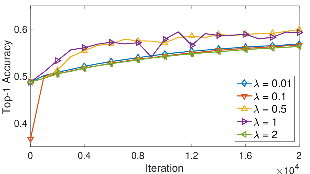
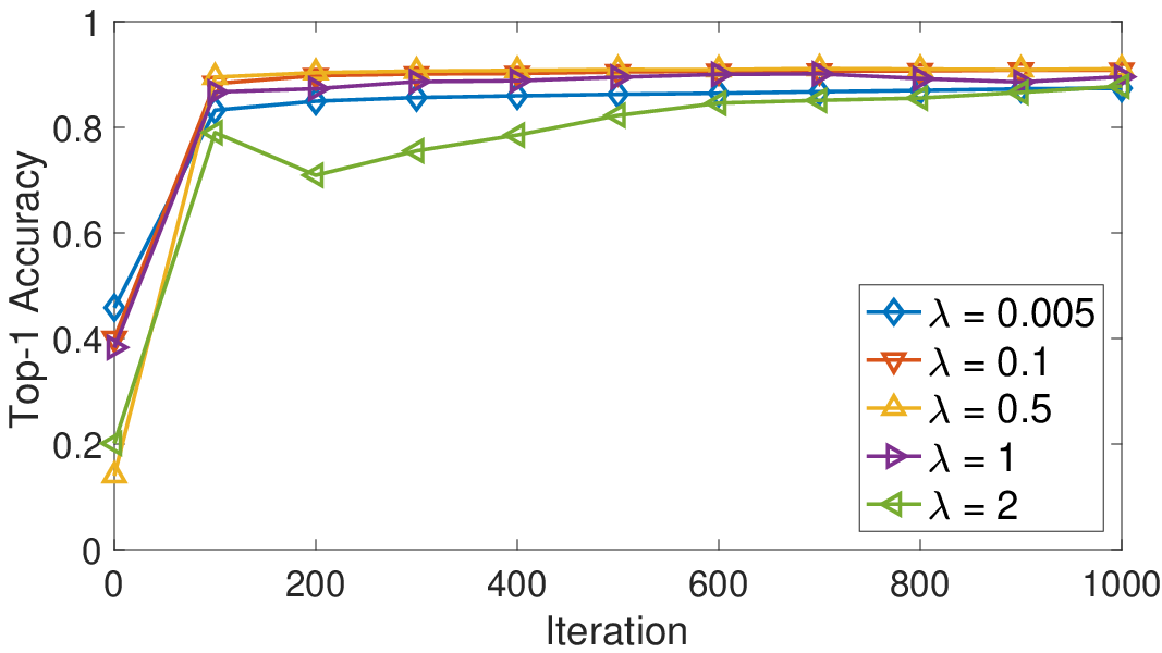
Impact of $\lambda$. Here we show how the performance of the proposed algorithm on the two datasets are affected by the choice of the penalty parameter $\lambda$. We use sign-flipping attack with $\varepsilon=-3$ in the numerical experiments, and the number of Byzantine workers is $q=4$. The parameters $\beta$, $\alpha_{0}^{k}$ and $\alpha_{i}^{k}$ are hand-tuned to the best. As depicted in Figure 6, on both datasets, the performance of Stochastic ADMM degrades when $\lambda$ is too small. The reason is that, when $\lambda$ is too small the regular workers are rely more on their local data, leading to deficiency of the distributed learning system [28]. Meanwhile, $\lambda$ being too large also leads to worse performance.

Non-i.i.d. data. To demonstrate the robustness of the proposed algorithm against Byzantine attacks on non-i.i.d. data, we redistribute the MNIST dataset by letting every two workers share one digit. All Byzantine workers $j$ choose one regular worker indexed by $p$, and send $u_{j}^{k+1}=x_{p}^{k+1}$ to the master at every iteration $k$. When the number of Byzantine workers is $q=4$, the best reachable accuracy is around 0.8, because of the absence of two handwriting digits’ data. Similarly, when the number of Byzantine workers is $q=8$, the best reachable accuracy is around 0.6. Here, we set the parameters of Stochastic ADMM as $\lambda=0.8$, $\beta=0.2$, $\alpha_{0}^{k}=\frac{1}{4+10\sqrt{k}}$, and $\alpha_{i}^{k}=\frac{1}{0.2+10\sqrt{k}}.$ when $q=4$. As shown in Figure 7(a), Median fails, Stochastic ADMM are close to Ideal SGD and outperforms all the other Byzantine-robust algorithms. When the number of Byzantine worker increases to $q=8$, in Stochastic ADMM, we set $\lambda=0.5$, $\beta=3$, $\alpha_{0}^{k}=\frac{1}{60+500\sqrt{k}}$, and $\alpha_{i}^{k}=\frac{1}{3+500\sqrt{k}}$. As depicted in Figure 7(b), Geometric median and Median fail because the stochastic gradients of regular worker $p$ dominate, such that only one digit can be recognized. Stochastic ADMM and RSA both work well, but Stochastic ADMM converges faster than RSA.

We proposed a stochastic ADMM to deal with the distributed learning problem under Byzantine attacks. We considered a TV norm-penalized approximation formulation to handle Byzantine attacks. Theoretically, we proved that the stochastic ADMM converges in expectation to a bounded neighborhood of the optimum at an $O(1/k)$-rate under mild assumptions. Numerically, we compared the proposed algorithm with other Byzantine-robust algorithms on two real datasets, showing the competitive performance of the Byzantine-robust stochastic ADMM.

References

• [1] R. Agrawal and R. Srikant. “Privacy-preserving Data Mining," Proceedings of ACM SIGMOD, 2000.
• [2] S. Sicari, A. Rizzardi, L. Grieco, and A. Coen-Porisini, “Security, Privacy and Trust in Internet of Things: The Road Ahead,” Computer Networks, vol. 76, pp. 146–164, 2015.
• [3] L. Zhou, K. Yeh, G. Hancke, Z. Liu, and C. Su, “Security and Privacy for the Industrial Internet of Things: An Overview of Approaches to Safeguarding Endpoints," IEEE Signal Processing Magazine, vol. 35, no. 5, pp. 76–87, 2018.
• [4] J. Konecny, H. McMahan, and D. Ramage, “Federated Optimization: Distributed Optimization Beyond the Datacenter,” arXiv: 1511.03575, 2015.
• [5] J. Konecny, H. McMahan, F. Yu, P. Richtarik, A. Suresh, and D. Bacon, “Federated Learning: Strategies for Improving Communication Efficiency,” arXiv: 1610.05492, 2016.
• [6] P. Kairouz and H. McMahan. “Advances and Open Problems in Federated Learning," Foundations and Trends in Machine Learning, vol. 14, no. 1, 2021.
• [7] L. Lamport, R. Shostak, and M. Pease, “The Byzantine Generals Problem,” ACM Transactions on Programming Languages and Systems, vol. 4, no. 3, pp. 382–401, 1982.
• [8] N. Lynch, Distributed Algorithms, Morgan Kaufmann Publishers, San Francisco, USA, 1996.
• [9] A. Vempaty, L. Tong, and P. K. Varshney, “Distributed Inference with Byzantine Data: State-of-the-Art Review on Data Falsification Attacks." IEEE Signal Processing Magazine, vol. 30, no. 5, pp. 65–75, 2013.
• [10] Y. Chen, S. Kar, and J. M. F. Moura, “The Internet of Things: Secure Distributed Inference." IEEE Signal Processing Magazine, vol. 35, no. 5, pp. 64–75, 2018.
• [11] P. Blanchard, E. M. E. Mhamdi, R. Guerraoui, and J. Stainer, “Machine Learning with Adversaries: Byzantine Tolerant Gradient Descent,” Proceedings of NeurIPS, 2017.
• [12] S. Li, Y. Cheng, W. Wang, Y. Liu, and T. Chen, “Abnormal Client Behavior Detection in Federated Learning,” arXiv: 1910.09933, 2019.
• [13] S. Li, Y. Cheng, W. Wang, Y. Liu, and T. Chen, “Learning to Detect Malicious Clients for Robust Federated Learning,” arXiv: 2002.00211, 2020.
• [14] N. Ravi and A. Scaglione, “Detection and Isolation of Adversaries in Decentralized Optimization for Non-Strongly Convex Objectives,” Proceedings of IFAC Workshop on Distributed Estimation and Control in Networked Systems, 2019.
• [15] D. Alistarh, Z. Allen-Zhu, and J. Li, “Byzantine Stochastic Gradient Descent,” Proceedings of NeuIPS, 2018.
• [16] Z. Allen-Zhu, F. Ebrahimianghazani, J. Li, and D. Alistarh, “Byzantine-Resilient Non-Convex Stochastic Gradient Descent,” Proceedings of ICLR, 2021.
• [17] L. Chen, H. Wang, Z. Charles, and D. Papailiopoulos, “DRACO: Byzantine-resilient Distributed Training via Redundant Gradients,” Proceedings of ICML, 2018.
• [18] Y. Chen, L. Su, and J. Xu, “Distributed Statistical Machine Learning in Adversarial Settings: Byzantine Gradient Descent,” Proceedings of the ACM on Measurement and Analysis of Computing Systems, 2018.
• [19] C. Xie, O. Koyejo, and I. Gupta, “Generalized Byzantine Tolerant SGD,” arXiv: 1802.10116, 2018.
• [20] X. Cao and L. Lai, “Distributed Approximate Newton’s Method Robust to Byzantine Attackers," IEEE Transactions on Signal Processing, vol. 68, pp. 6011–6025, 2020.
• [21] D. Yin, Y. Chen, K. Ramchandran, and P. Bartlett, “Byzantine-robust Distributed Learning: Towards Optimal Statistical Rates,” Proceedings of ICML, 2018.
• [22] C. Xie, S. Koyejo, and I. Gupta, “Zeno: Distributed Stochastic Gradient Descent with Suspicion-based Fault-tolerance,” Proceedings of ICML, 2019.
• [23] C. Xie, O. Koyejo, and I. Gupta, “Phocas: Dimensional Byzantine-resilient Stochastic Gradient Descent,” arXiv: 1805.09682, 2018.
• [24] E. M. E. Mhamdi, R. Guerraoui, and S. Rouault, “The Hidden Vulnerability of Distributed Learning in Byzantium,” Proceedings of ICML, 2018.
• [25] K. Hsieh, A. Phanishayee, O. Mutlu, and P. B. Gibbons, “The Non-IID Data Quagmire of Decentralized Machine Learning,” Proceedings of ICML, 2020.
• [26] L. He, S. P. Karimireddy, and M. Jaggi, “Byzantine-robust Learning on Heterogeneous Datasets via Resampling,” arXiv: 2006.09365, 2020.
• [27] J. Peng, Z. Wu, Q. Ling, and T. Chen, “Byzantine-Robust Variance-Reduced Federated Learning over Distributed Non-i.i.d. Data,” arXiv: 2009.08161, 2020.
• [28] L. Li, W. Xu, T. Chen, G. Giannakis, and Q. Ling, “RSA: Byzantine-robust Stochastic Aggregation Methods for Distributed Learning from Heterogeneous Datasets,” Proceedings of AAAI, 2019.
• [29] Z. Wu, Q. Ling, T. Chen, and G. Giannakis, “Federated Variance-Reduced Stochastic Gradient Descent with Robustness to Byzantine Attacks,” IEEE Transactions on Signal Processing, vol. 68, pp. 4583–4596, 2020.
• [30] E. M. E. Mhamdi, R. Guerraoui, and S. Rouault, “Distributed Momentum for Byzantine-resilient Learning,” Proceedings of ICLR, 2021.
• [31] P. Khanduri, S. Bulusu, P. Sharma, and P. Varshney, “Byzantine Resilient Non-Convex SVRG with Distributed Batch Gradient Computations,” arXiv: 1912.04531, 2019.
• [32] S. P. Karimireddy, L. He, and M. Jaggi, “Learning from History for Byzantine Robust Optimization,” Proceedings of ICML, 2021.
• [33] G. Damaskinos, E. M. E. Mhamdi, R. Guerraoui, R. Patra, and M. Taziki, “Asynchronous Byzantine Machine Learning (the Case of SGD),” Proceedings of ICML, 2018.
• [34] Y. Yang and W. Li, “BASGD: Buffered Asynchronous SGD for Byzantine Learning,” arXiv: 2003.00937, 2020.
• [35] C. Xie, S. Koyejo, and I. Gupta, “Zeno++: Robust Fully Asynchronous SGD,” Proceedings of ICML, 2020.
• [36] D. Yin, Y. Chen, R. Kannan, and P. Bartlett, “Defending Against Saddle Point Attack in Byzantine-Robust Distributed Learning,” Proceedings of ICML, 2019.
• [37] Z. Yang and W. U. Bajwa, “ByRDiE: Byzantine-Resilient Distributed Coordinate Descent for Decentralized Learning,” IEEE Transactions on Signal and Information Processing over Networks, vol. 5, no. 4, pp. 611–627, 2019.
• [38] Z. Yang and W. U. Bajwa, “BRIDGE: Byzantine-resilient Decentralized Gradient Descent,” arXiv: 1908.08098, 2019.
• [39] S. Guo, T. Zhang, X. Xie, L. Ma, T. Xiang, and Y. Liu, “Towards Byzantine-resilient Learning in Decentralized Systems,” arXiv: 2002.08569, 2020
• [40] J. Peng, W. Li, and Q. Ling, “Byzantine-robust Decentralized Stochastic Optimization over Static and Time-varying Networks,” Signal Processing, vol. 183, no. 108020, 2021.
• [41] H. Ouyang, N. He, and A. Gray, “Stochastic ADMM for Nonsmooth Optimization,” arXiv: 1211.0632, 2012.
• [42] W. Ben-Ameur, P. Bianchi, and J. Jakubowicz, “Robust Distributed Consensus Using Total Variation,” IEEE Transactions on Automatic Control, vol. 61, no. 6, pp. 1550–1564, 2016.
• [43] Y. Nesterov, Introductory Lectures on Convex Optimization: A Basic Course, Springer, Boston, USA, 2004.
Appendix A Proof of Proposition 1
The proof of Proposition 1 relies on the following Lemma.
Lemma 2.
Let {z1∗,z2∗}=arg⁡minz1,z2∈ℝ⁡λ​|z1−z2|+12​(z1−a1)2+12​(z2−a2)2\{z_{1}^{*},z_{2}^{*}\}={\arg\min}_{z_{1},z_{2}\in\mathbb{R}}~\lambda|z_{1}-z_{2}|+\frac{1}{2}(z_{1}-a_{1})^{2}+\frac{1}{2}(z_{2}-a_{2})^{2}, where λ,a1,a2∈ℝ\lambda,a_{1},a_{2}\in\mathbb{R}. Then
z1∗+z2∗=a1+a2andz1∗−a1=projλ​(a2−a12).z_{1}^{*}+z_{2}^{*}=a_{1}+a_{2}\quad\text{and}\quad z_{1}^{*}-a_{1}=\mathrm{proj}_{\lambda}\left(\frac{a_{2}-a_{1}}{2}\right). (19)
Proof.
Note that {z1∗,z2∗}\{z_{1}^{*},z_{2}^{*}\} together with their difference Δ∗=z1∗−z2∗\Delta^{*}=z_{1}^{*}-z_{2}^{*} is also optimal to the bi-level minimization problem
minΔ∈ℝ\displaystyle\min_{\Delta\in\mathbb{R}} minz1,z2∈ℝ⁡λ​|z1−z2|+12​(z1−a1)2+12​(z2−a2)2,\displaystyle\min_{z_{1},z_{2}\in\mathbb{R}}~\lambda|z_{1}-z_{2}|+\frac{1}{2}(z_{1}-a_{1})^{2}+\frac{1}{2}(z_{2}-a_{2})^{2},
s.t.z1−z2=Δ.\displaystyle\quad s.t.\quad z_{1}-z_{2}=\Delta.
That is, we first optimize the constrained minimization problem with an artificially imposed constraint z1−z2=Δz_{1}-z_{2}=\Delta over {z1,z2}\{z_{1},z_{2}\}, and then optimize over Δ\Delta.
For the inner-level constrained minimization problem, from its KKT (Karush-Kuhn-Tucker) conditions we know the minimizer is {z1∗=a1+a2+Δ2,z2∗=a1+a2−Δ2}\{z_{1}^{*}=\frac{a_{1}+a_{2}+\Delta}{2},z_{2}^{*}=\frac{a_{1}+a_{2}-\Delta}{2}\}, and accordingly, the optimal value is λ​|Δ|+(Δ−(a1−a2))24\lambda|\Delta|+\frac{(\Delta-(a_{1}-a_{2}))^{2}}{4}. Therefore, for the outer-level unconstrained minimization problem, from its KKT conditions we know the minimizer can be written as Δ∗=(a1−a2)−proj2​λ​(a1−a2)\Delta^{*}=(a_{1}-a_{2})-\mathrm{proj}_{2\lambda}(a_{1}-a_{2}). Substituting this result to {z1∗=a1+a2+Δ∗2,z2∗=a1+a2−Δ2∗}\{z_{1}^{*}=\frac{a_{1}+a_{2}+\Delta^{*}}{2},z_{2}^{*}=\frac{a_{1}+a_{2}-\Delta}{2}^{*}\} yields z1∗=a1+projλ​(a2−a12)z_{1}^{*}=a_{1}+\mathrm{proj}_{\lambda}\left(\frac{a_{2}-a_{1}}{2}\right) and z2∗=a2+projλ​(a1−a22)z_{2}^{*}=a_{2}+\mathrm{proj}_{\lambda}\left(\frac{a_{1}-a_{2}}{2}\right). From them we obtain (19) and complete the proof.
Now we begin to prove Proposition 1. Since (8b) is separable with respect to ii, it is equivalent to
{zk+1​(i,0),zk+1​(0,i)}\displaystyle~\left\{z^{k+1}(i,0),z^{k+1}(0,i)\right\} (20)
=\displaystyle= arg⁡minz⁡(i,0),z⁡(0,i)​λ​‖z⁡(0,i)−z⁡(i,0)‖1+β2​‖z⁡(i,0)−(x0k+1−1β​ηk​(i,0))‖2+β2​‖z⁡(0,i)−(xik+1−1β​ηk​(0,i))‖2,\displaystyle~{\arg\min}_{z(i,0),z(0,i)}\lambda\|z(0,i)-z(i,0)\|_{1}+\frac{\beta}{2}\big\|z(i,0)-\big(x_{0}^{k+1}-\frac{1}{\beta}\eta^{k}(i,0)\big)\big\|^{2}+\frac{\beta}{2}\big\|z(0,i)-\big(x_{i}^{k+1}-\frac{1}{\beta}\eta^{k}(0,i)\big)\big\|^{2},
According to Lemma 2, (20) leads to
zk+1​(0,i)+zk+1​(i,0)\displaystyle{z^{k+1}(0,i)+z^{k+1}(i,0)} =xik+1+x0k+1−ηk​(0,i)+ηk​(i,0)β,\displaystyle={x_{i}^{k+1}+x_{0}^{k+1}}-\frac{\eta^{k}(0,i)+\eta^{k}(i,0)}{\beta}, (21a)
zk+1​(i,0)−(x0k+1−1β​ηk​(i,0))\displaystyle z^{k+1}(i,0)-\big(x_{0}^{k+1}-\frac{1}{\beta}\eta^{k}(i,0)\big) =projλ/β​((ηk​(i,0)−ηk​(0,i))/β+xik+1−x0k+12).\displaystyle=\mathrm{proj}_{\lambda/\beta}\left(\frac{(\eta^{k}(i,0)-\eta^{k}(0,i))/\beta+x_{i}^{k+1}-x_{0}^{k+1}}{2}\right). (21b)
From (8c) and (21a) we have
ηk+1​(0,i)+ηk+1​(i,0)=0,\eta^{k+1}(0,i)+\eta^{k+1}(i,0)=0, (22)
which is regardless of the initialization of η\eta. If we further initialize η0​(i,0)=−η0​(0,i)\eta^{0}(i,0)=-\eta^{0}(0,i), for simplicity we can define for any k≥0k\geq 0 that
ηik:=ηk​(i,0)=−ηk​(0,i).\eta^{k}_{i}:=\eta^{k}(i,0)=-\eta^{k}(0,i).
With this notation, we rewrite (8c) as
ηik+1=ηik+β⁡(zk+1​(i,0)−x0k+1)=projλ​(ηik+β2​(xik+1−x0k+1)),\displaystyle\eta^{k+1}_{i}=\eta^{k}_{i}+\beta(z^{k+1}(i,0)-x_{0}^{k+1})=\mathrm{proj}_{\lambda}\left(\eta^{k}_{i}+\frac{\beta}{2}(x^{k+1}_{i}-x^{k+1}_{0})\right), (23)
where the last equality is from (21b).
Next we simplify the updates of xik+1x_{i}^{k+1} and x0k+1x_{0}^{k+1} in (11). From (8c), we have
β​xik−β​zk​(0,i)−ηk​(0,i)\displaystyle\beta x_{i}^{k}-\beta z^{k}(0,i)-\eta^{k}(0,i) =ηk−1​(0,i)−ηk​(0,i)−ηk​(0,i)=2​ηik−ηik−1,\displaystyle=\eta^{k-1}(0,i)-\eta^{k}(0,i)-\eta^{k}(0,i)=2\eta^{k}_{i}-\eta^{k-1}_{i},
which simplifies (11) to
xik+1\displaystyle x^{k+1}_{i} =xik−αik​(F′​(xik,ξik)+2​ηik−ηik−1),\displaystyle=x_{i}^{k}-\alpha_{i}^{k}\left(F^{\prime}(x_{i}^{k},\xi^{k}_{i})+2\eta^{k}_{i}-\eta^{k-1}_{i}\right), (24)
x0k+1\displaystyle x^{k+1}_{0} =x0k−α0k​(f0′​(x0k)−∑i∈ℛ(2​ηik−ηik−1)).\displaystyle=x_{0}^{k}-\alpha_{0}^{k}\Big(f_{0}^{\prime}(x_{0}^{k})-\sum_{i\in\mathcal{R}}(2\eta^{k}_{i}-\eta^{k-1}_{i})\Big). (25)
This completes the proof.
Appendix B Supporting Lemmas
Lemma 3 (Optimality conditions of (6)).
The sufficient and necessary optimality conditions of (6) are
{𝔼[F′(xi∗,ξi)]=η∗(0,i),f′0(x0∗)=∑i∈ℛη∗(i,0),η∗(0,i)=−λgi∗,η∗(i,0)=λgi∗,z∗(i,0)=x0∗,z∗(0,i)=xi∗,\begin{cases}\mathbb{E}[F^{\prime}({x_{i}^{*}},\xi_{i})]=\eta^{*}(0,i),\quad f^{\prime}_{0}(x_{0}^{*})=\sum_{i\in\mathcal{R}}\eta^{*}(i,0),\\ \eta^{*}(0,i)=-\lambda g_{i}^{*},\quad\eta^{*}(i,0)=\lambda g_{i}^{*},\\ z^{*}(i,0)=x_{0}^{*},\quad z^{*}(0,i)=x_{i}^{*},\end{cases} (26)
for all i∈ℛi\in\mathcal{R}, where gi∗∈s​g​n​(z∗​(0,i)−z∗​(i,0))g_{i}^{*}\in{sgn}(z^{*}(0,i)-z^{*}(i,0)). In particular, defining ηi∗:=η∗​(i,0)\eta_{i}^{*}:=\eta^{*}(i,0), we have for all i∈ℛi\in\mathcal{R} that
f0′(x0∗)=∑i∈ℛηi∗,𝔼[F′(xi∗,ξi)]=−ηi∗,andηi∗=λgi∗∈[−λ,λ]d.\displaystyle f^{\prime}_{0}(x_{0}^{*})=\sum_{i\in\mathcal{R}}\eta_{i}^{*},\quad\mathbb{E}[F^{\prime}({x_{i}^{*}},\xi_{i})]=-\eta_{i}^{*},\quad\text{and}\quad\eta_{i}^{*}=\lambda g_{i}^{*}\in[-\lambda,\lambda]^{d}. (27)
The KKT conditions of (6) are given by
{𝔼[F′(xi∗,ξi)]−η∗(0,i)=0,f′0(x0∗)+∑i(−η∗(i,0)=0,0∈λ∂z∗​(0,i)∥z∗(0,i)−z∗(i,0)∥1+η∗(0,i),0∈λ∂z∗​(i,0)∥z∗(0,i)−z∗(i,0)∥1+η∗(i,0),z∗(i,0)−x0∗=0,z∗(0,i)−xi∗=0,\displaystyle\begin{cases}\mathbb{E}[F^{\prime}({x_{i}^{*}},\xi_{i})]-\eta^{*}(0,i)=0,\quad f^{\prime}_{0}(x_{0}^{*})+\sum_{i}\big(-\eta^{*}(i,0)=0,\\ 0\in\lambda\partial_{z^{*}(0,i)}\|z^{*}(0,i)-z^{*}(i,0)\|_{1}+\eta^{*}(0,i),\quad 0\in\lambda\partial_{z^{*}(i,0)}\|z^{*}(0,i)-z^{*}(i,0)\|_{1}+\eta^{*}(i,0),\\ z^{*}(i,0)-x_{0}^{*}=0,\quad z^{*}(0,i)-x_{i}^{*}=0,\end{cases}
where ∂z∗​(0,i)(⋅)\partial_{z^{*}(0,i)}(\cdot) and ∂z∗​(i,0)(⋅)\partial_{z^{*}(i,0)}(\cdot) denote the sets of subgradients. Applying the definition of the element-wise sign function s​g​n​(⋅)sgn(\cdot) yields (26). Further noticing ηi∗:=η∗​(i,0)=−η∗​(i,0)\eta_{i}^{*}:=\eta^{*}(i,0)=-\eta^{*}(i,0), we obtain (27).
Lemma 4 (Theorem 2.1.12, [43]).
With Assumptions 1 and 2, for any xix_{i} and x0x_{0}, it holds
⟨Fi′​(xi)−Fi′​(xi∗),xi−xi∗⟩≥1μi+Li​‖Fi′​(xi)−Fi′​(xi∗)‖2+μi​Liμi+Li​‖xi−xi∗‖2,\displaystyle\langle F^{\prime}_{i}(x_{i})-F^{\prime}_{i}(x_{i}^{*}),x_{i}-x_{i}^{*}\rangle\geq\frac{1}{\mu_{i}+L_{i}}\|F^{\prime}_{i}(x_{i})-F^{\prime}_{i}(x_{i}^{*})\|^{2}+\frac{\mu_{i}L_{i}}{\mu_{i}+L_{i}}\|x_{i}-x_{i}^{*}\|^{2},\quad (28)
⟨f0′​(x0)−f0′​(x0∗),x0−x0∗⟩≥1μ0+L0​‖f0′​(x0)−f0′​(x0∗)‖2+μ0​L0μ0+L0​‖x0−x0∗‖2.\displaystyle\langle f^{\prime}_{0}(x_{0})-f^{\prime}_{0}(x_{0}^{*}),x_{0}-x_{0}^{*}\rangle\geq\frac{1}{\mu_{0}+L_{0}}\|f^{\prime}_{0}(x_{0})-f^{\prime}_{0}(x_{0}^{*})\|^{2}+\frac{\mu_{0}L_{0}}{\mu_{0}+L_{0}}\|x_{0}-x_{0}^{*}\|^{2}. (29)
Lemma 5.
With the simplified updates (12), (13), and (14), it holds for any regular worker i∈ℛi\in\mathcal{R} that
⟨ηik+1−ηi∗,x0k+1−xik+1⟩≤\displaystyle\langle\eta_{i}^{k+1}-\eta_{i}^{*},x_{0}^{k+1}-x_{i}^{k+1}\rangle\leq −2β​⟨ηik+1−ηi∗,ηik+1−ηik⟩=1β​(‖ηik−ηi∗‖2−‖ηik+1−ηi∗‖2−‖ηik+1−ηik‖2),\displaystyle~-\frac{2}{\beta}\langle\eta_{i}^{k+1}-\eta_{i}^{*},\eta_{i}^{k+1}-\eta_{i}^{k}\rangle=\frac{1}{\beta}\left(\|\eta_{i}^{k}-\eta_{i}^{*}\|^{2}-\|\eta_{i}^{k+1}-\eta_{i}^{*}\|^{2}-\|\eta_{i}^{k+1}-\eta_{i}^{k}\|^{2}\right), (30)
⟨ηik+1,x0k+1−xik+1⟩≤\displaystyle\langle\eta_{i}^{k+1},x_{0}^{k+1}-x_{i}^{k+1}\rangle\leq −2β​⟨ηik+1,ηik+1−ηik⟩=1β​(‖ηik‖2−‖ηik+1‖2−‖ηik+1−ηik‖2).\displaystyle~-\frac{2}{\beta}\langle\eta_{i}^{k+1},\eta_{i}^{k+1}-\eta_{i}^{k}\rangle=\frac{1}{\beta}\left(\|\eta_{i}^{k}\|^{2}-\|\eta_{i}^{k+1}\|^{2}-\|\eta_{i}^{k+1}-\eta_{i}^{k}\|^{2}\right). (31)
We first show the inequality in (30), and then modify it to prove (31). The relationships derived during the proof of Lemma 2 are useful here. Since ηik:=ηk​(i,0)=−ηk​(0,i)\eta^{k}_{i}:=\eta^{k}(i,0)=-\eta^{k}(0,i), the right-hand side of (21b) is exactly 1β​ηik+1\frac{1}{\beta}\eta_{i}^{k+1}. Combining this fact with (21a) yields
zk+1​(i,0)=x0k+1+1β​(ηik+1−ηik),zk+1​(0,i)=xik+1−1β​(ηik+1−ηik).z^{k+1}(i,0)=x_{0}^{k+1}+\frac{1}{\beta}\big(\eta_{i}^{k+1}-\eta_{i}^{k}\big),\quad z^{k+1}(0,i)=x_{i}^{k+1}-\frac{1}{\beta}\big(\eta_{i}^{k+1}-\eta_{i}^{k}\big). (32)
Recall that in (20), we minimize the function
λ​‖z⁡(0,i)−z⁡(i,0)‖1+β2​‖z⁡(i,0)−(x0k+1−1β​ηik)‖2+β2​‖z⁡(0,i)−(xik+1+1β​ηik)‖2,\lambda\|z(0,i)-z(i,0)\|_{1}+\frac{\beta}{2}\big\|z(i,0)-\big(x_{0}^{k+1}-\frac{1}{\beta}\eta^{k}_{i}\big)\big\|^{2}+\frac{\beta}{2}\big\|z(0,i)-\big(x_{i}^{k+1}+\frac{1}{\beta}\eta^{k}_{i}\big)\big\|^{2},
with respect to [z⁡(i,0);z⁡(0,i)]∈ℝ2​d\big[z(i,0);z(0,i)\big]\in\mathbb{R}^{2d}. From the first order optimality condition, there exists a subgradient of λ​‖z⁡(0,i)−z⁡(i,0)‖1\lambda\|z(0,i)-z(i,0)\|_{1} at [zk+1​(0,i);zk+1​(i,0)]\big[z^{k+1}(0,i);z^{k+1}(i,0)\big], denoted as [λ​gik+1;−λ​gik+1]∈[−λ,λ]2​d[\lambda g_{i}^{k+1};-\lambda g_{i}^{k+1}]\in[-\lambda,\lambda]^{2d}, such that
0=λ​gik+1+β⁡(zk+1​(0,i)−(xik+1+1β​ηik))=λ​gik+1−ηk+1.0=\lambda g_{i}^{k+1}+\beta\big(z^{k+1}(0,i)-(x_{i}^{k+1}+\frac{1}{\beta}\eta^{k}_{i})\big)=\lambda g_{i}^{k+1}-\eta^{k+1}. (33)
Applying the definition of subgradient of λ​‖z⁡(0,i)−z⁡(i,0)‖1\lambda\|z(0,i)-z(i,0)\|_{1} at points [zk+1​(0,i);zk+1​(i,0)]\big[z^{k+1}(0,i);z^{k+1}(i,0)\big] and [z∗​(0,i);z∗​(i,0)]\big[z^{*}(0,i);z^{*}(i,0)\big] gives
λ​‖z∗​(0,i)−z∗​(i,0)‖1≥\displaystyle\lambda\|z^{*}(0,i)-z^{*}(i,0)\|_{1}\geq λ​‖zk+1​(0,i)−zk+1​(i,0)‖1\displaystyle~\lambda\|z^{k+1}(0,i)-z^{k+1}(i,0)\|_{1}
+⟨[(λgik+1;−λgik+1]),[z∗(0,i)−zk+1(0,i);z∗(i,0)−zk+1(i,0)]⟩,\displaystyle~+\big\langle[(\lambda g_{i}^{k+1};-\lambda g_{i}^{k+1}]),\big[z^{*}(0,i)-z^{k+1}(0,i);z^{*}(i,0)-z^{k+1}(i,0)\big]\big\rangle, (34)
λ​‖zk+1​(0,i)−zk+1​(i,0)‖1≥\displaystyle\lambda\|z^{k+1}(0,i)-z^{k+1}(i,0)\|_{1}\geq λ​‖z∗​(0,i)−z∗​(i,0)‖1\displaystyle~\lambda\|z^{*}(0,i)-z^{*}(i,0)\|_{1}
+⟨[λ​gi∗;−λ​gi∗],[zk+1​(0,i)−z∗​(0,i);zk+1​(i,0)−z∗​(i,0)]⟩,\displaystyle~+\big\langle[\lambda g_{i}^{*};-\lambda g_{i}^{*}],\big[z^{k+1}(0,i)-z^{*}(0,i);z^{k+1}(i,0)-z^{*}(i,0)\big]\big\rangle, (35)
where gi∗=ηi∗λg_{i}^{*}=\frac{\eta_{i}^{*}}{\lambda} is defined in Lemma 3. Summing up (34) and (35), we have
0≥⟨λ​gik+1−λ​gi∗,zk+1​(i,0)−zk+1​(0,i)⟩=⟨ηk+1−η∗,x0k+1−xik+1+2β​(ηik+1−ηik)⟩,0\geq\big\langle\lambda g_{i}^{k+1}-\lambda g_{i}^{*},z^{k+1}(i,0)-z^{k+1}(0,i)\big\rangle=\big\langle\eta^{k+1}-\eta^{*},x_{0}^{k+1}-x_{i}^{k+1}+\frac{2}{\beta}\big(\eta_{i}^{k+1}-\eta_{i}^{k}\big)\big\rangle,
where the last equality comes from (32) and (33). Rearranging the terms gives (30).
Further note that [λ​gi∗;−λ​gi∗][\lambda g_{i}^{*};-\lambda g_{i}^{*}] in (35) can be replaced by any subgradient of λ​‖z⁡(0,i)−z⁡(i,0)‖1\lambda\|z(0,i)-z(i,0)\|_{1} at [z∗​(0,i);z∗​(i,0)]\big[z^{*}(0,i);z^{*}(i,0)\big]. We hence replace it by [0;0][0;0], and then obtain (31).
Appendix C Proof of Theorem 1
Restatement of Theorem 1. Suppose Assumptions 1, 2, and 3 hold. let λ≥λ0\lambda\geq\lambda_{0} and the stepsizes be
α0k=min⁡{1c​k+m​β,A},αik=min⁡{1c​k+β,A},∀i∈ℛ,\alpha_{0}^{k}=\min\left\{\frac{1}{ck+m\beta},A\right\},\quad\alpha_{i}^{k}=\min\left\{\frac{1}{ck+\beta},A\right\},\ \forall i\in\mathcal{R},
for some positive constants c<min{μ0​L0μ0+L0,μi​Liμi+Li:i∈ℛ}c<\min\left\{\frac{\mu_{0}L_{0}}{\mu_{0}+L_{0}},\frac{\mu_{i}L_{i}}{\mu_{i}+L_{i}}:i\in\mathcal{R}\right\}, β\beta, and A≤min{1μ0+L0,1μi+Li:i∈ℛ}{A}\leq\min\left\{\frac{1}{\mu_{0}+L_{0}},\frac{1}{\mu_{i}+L_{i}}:i\in\mathcal{R}\right\}. Define constants
c0\displaystyle c_{0} =min{c+(m−1)β,μ0​L0μ0+L0,μi​Liμi+Li:i∈ℛ},\displaystyle=\min\bigg\{c+(m-1)\beta,\frac{\mu_{0}L_{0}}{\mu_{0}+L_{0}},\frac{\mu_{i}L_{i}}{\mu_{i}+L_{i}}:i\in\mathcal{R}\bigg\},
c1\displaystyle c_{1} =9​d​(μ0+L0)μ0​L0​λ2​q2,\displaystyle=\frac{9d(\mu_{0}+L_{0})}{\mu_{0}L_{0}}\lambda^{2}q^{2},
c2\displaystyle c_{2} =[2​(4​r+3​q)2+64​r+16​(m−1)​β​(r2​β+∑i(1μi+1Li))]​λ2​d+4​∑iδi2.\displaystyle=\left[2(4r+3q)^{2}+64r+16(m-1)\beta\left(\frac{r}{2\beta}+\sum_{i}\bigg(\frac{1}{\mu_{i}}+\frac{1}{L_{i}}\bigg)\right)\right]\lambda^{2}d+4\sum_{i}\delta_{i}^{2}.
Also denote Vk=𝔼​‖x0k−x0∗‖2+∑i∈ℛ(𝔼​‖xik−xi∗‖2+2​αik−1β​‖ηik−1−ηi∗‖2)V^{k}=\mathbb{E}\|x_{0}^{k}-x_{0}^{*}\|^{2}+\sum_{i\in\mathcal{R}}\big(\mathbb{E}\|x_{i}^{k}-x_{i}^{*}\|^{2}+\frac{2\alpha_{i}^{k-1}}{\beta}\|\eta_{i}^{k-1}-\eta_{i}^{*}\|^{2}\big). Then we have
Vk+1≤{Vk(1−c0αk0)+c1αk0+c2(αki)2,k>k0,Vk(1−c0A)+Ac1+A2c2,k≤k0,\displaystyle V^{k+1}\leq\begin{cases}V^{k}(1-c_{0}\alpha^{k}_{0})+c_{1}\alpha^{k}_{0}+c_{2}(\alpha^{k}_{i})^{2},\quad&k>k_{0},\\ V^{k}(1-c_{0}A)+{A}c_{1}+{A}^{2}c_{2},\quad&k\leq k_{0},\end{cases} (36)
where k0=min⁡{k:1c​k+β<A}k_{0}=\min\{k:\frac{1}{ck+\beta}<A\}. Consequently, it holds
Vk≤{V0(1−cA)k+1+c1+A​c2c0,k≤k0,Cc⁡(k−1)+m​β+c1c0,k>k0,V^{k}\leq\begin{cases}V^{0}(1-cA)^{k+1}+\frac{c_{1}+{A}c_{2}}{c_{0}},\quad&k\leq k_{0},\\ \frac{C}{c(k-1)+m\beta}+\frac{c_{1}}{c_{0}},\quad&k>k_{0},\end{cases} (37)
with
C=max⁡{(c​k0+m​βc​k0+β)2​c2c0−c,(c​k0+m​β)​(V0​(1−c0​A)k0+1+A​c2c0)}.C=\max\left\{\left(\frac{ck_{0}+m\beta}{ck_{0}+\beta}\right)^{2}\frac{c_{2}}{c_{0}-c},(ck_{0}+m\beta)\left(V^{0}(1-c_{0}A)^{k_{0}+1}+\frac{Ac_{2}}{c_{0}}\right)\right\}.
Recall that the updates satisfy
x0k+1=\displaystyle x_{0}^{k+1}= x0k−α0k​(f0′​(x0k)−∑i∈ℛ(2​ηik−ηik−1)−∑j∈ℬ(2​ηjk−ηjk−1)),\displaystyle~x_{0}^{k}-\alpha_{0}^{k}\bigg(f^{\prime}_{0}(x_{0}^{k})-\sum_{i\in\mathcal{R}}\big(2\eta^{k}_{i}-\eta^{k-1}_{i}\big)-\sum_{j\in\mathcal{B}}\big(2\eta^{k}_{j}-\eta^{k-1}_{j}\big)\bigg), (38)
xik+1=\displaystyle x_{i}^{k+1}= xik−αik​(F′​(xik,ξik)+(2​ηik−ηik−1)),∀i∈ℛ,\displaystyle~x_{i}^{k}-\alpha_{i}^{k}\bigg(F^{\prime}(x_{i}^{k},\xi_{i}^{k})+\big(2\eta^{k}_{i}-\eta^{k-1}_{i}\big)\bigg),\forall i\in\mathcal{R}, (39)
ηik+1=\displaystyle\eta_{i}^{k+1}= projλ(ηik+β2(xik+1−x0k+1))∈[−λ,λ]d,∀i∈ℛandηjk+1∈[−λ,λ]d,∀j∈ℬ.\displaystyle~\mathrm{proj}_{\lambda}\left(\eta^{k}_{i}+\frac{\beta}{2}(x^{k+1}_{i}-x^{k+1}_{0})\right)\in[-\lambda,\lambda]^{d},\forall i\in\mathcal{R}\quad\text{and}\quad\eta_{j}^{k+1}\in[-\lambda,\lambda]^{d},\forall j\in\mathcal{B}. (40)
Step 1. At the master side, we have
𝔼​‖x0k+1−x0∗‖2​=(38)\displaystyle\mathbb{E}\|x_{0}^{k+1}-x_{0}^{*}\|^{2}\overset{\eqref{x0-adm-sim}}{=} 𝔼​‖x0k−x0∗‖2+(α0k)2​𝔼​‖f0′​(x0k)−∑i∈ℛ(2​ηik−ηik−1)−∑j∈ℬ(2​ηjk−ηjk−1)‖2\displaystyle~\mathbb{E}\|x_{0}^{k}-x_{0}^{*}\|^{2}+(\alpha_{0}^{k})^{2}\mathbb{E}\bigg\|f^{\prime}_{0}(x_{0}^{k})-\sum_{i\in\mathcal{R}}\big(2\eta^{k}_{i}-\eta^{k-1}_{i}\big)-\sum_{j\in\mathcal{B}}\big(2\eta^{k}_{j}-\eta^{k-1}_{j}\big)\bigg\|^{2}
−2​α0k​𝔼​⟨f0′​(x0k)−∑i∈ℛ(2​ηik−ηik−1)−∑j∈ℬ(2​ηjk−ηjk−1),x0k−x0∗⟩.\displaystyle~-2\alpha_{0}^{k}\mathbb{E}\bigg\langle f^{\prime}_{0}(x_{0}^{k})-\sum_{i\in\mathcal{R}}\big(2\eta^{k}_{i}-\eta^{k-1}_{i}\big)-\sum_{j\in\mathcal{B}}\big(2\eta^{k}_{j}-\eta^{k-1}_{j}\big),x_{0}^{k}-x_{0}^{*}\bigg\rangle. (41)
For the second term in (41), the inequality ‖a+b‖2≤2​‖a‖2+2​‖b‖2\|a+b\|^{2}\leq 2\|a\|^{2}+2\|b\|^{2} gives
𝔼​‖f0′​(x0k)−∑i∈ℛ(2​ηik−ηik−1)−∑j∈ℬ(2​ηjk−ηjk−1)‖2\displaystyle~\mathbb{E}\bigg\|f^{\prime}_{0}(x_{0}^{k})-\sum_{i\in\mathcal{R}}\big(2\eta^{k}_{i}-\eta^{k-1}_{i}\big)-\sum_{j\in\mathcal{B}}\big(2\eta^{k}_{j}-\eta^{k-1}_{j}\big)\bigg\|^{2}
=(27)\displaystyle\overset{\eqref{eq:opt}}{=} 𝔼​‖f0′​(x0k)−f0′​(x0∗)−∑i∈ℛ(2​ηik−ηik−1−ηi∗)−∑j∈ℬ(2​ηjk−ηjk−1)‖2\displaystyle~\mathbb{E}\bigg\|f^{\prime}_{0}(x_{0}^{k})-f^{\prime}_{0}(x_{0}^{*})-\sum_{i\in\mathcal{R}}\big(2\eta^{k}_{i}-\eta^{k-1}_{i}-\eta^{*}_{i}\big)-\sum_{j\in\mathcal{B}}\big(2\eta^{k}_{j}-\eta^{k-1}_{j}\big)\bigg\|^{2}
≤\displaystyle\leq 2​𝔼​‖f0′​(x0k)−f0′​(x0∗)‖2+2​𝔼​‖∑i∈ℛ(2​ηik−ηik−1−ηi∗)+∑j∈ℬ(2​ηjk−ηjk−1)‖2\displaystyle~2\mathbb{E}\big\|f^{\prime}_{0}(x_{0}^{k})-f^{\prime}_{0}(x_{0}^{*})\big\|^{2}+2\mathbb{E}\bigg\|\sum_{i\in\mathcal{R}}\big(2\eta^{k}_{i}-\eta^{k-1}_{i}-\eta^{*}_{i}\big)+\sum_{j\in\mathcal{B}}\big(2\eta^{k}_{j}-\eta^{k-1}_{j}\big)\bigg\|^{2}
≤(40)\displaystyle\overset{\eqref{eta-range}}{\leq} 2​𝔼​‖f0′​(x0k)−f0′​(x0∗)‖2+2​(4​r+3​q)2​λ2​d.\displaystyle~2\mathbb{E}\big\|f^{\prime}_{0}(x_{0}^{k})-f^{\prime}_{0}(x_{0}^{*})\big\|^{2}+2(4r+3q)^{2}\lambda^{2}d. (42)
Applying the inequality 2​⟨a,b⟩≤ϵ​‖a‖2+1ϵ​‖b‖22\langle a,b\rangle\leq\epsilon\|a\|^{2}+\frac{1}{\epsilon}\|b\|^{2} to the third term in (41) with ϵ=μ0​L0μ0+L0\epsilon=\frac{\mu_{0}L_{0}}{\mu_{0}+L_{0}} yields
−2​𝔼​⟨f0′​(x0k)−∑i∈ℛ(2​ηik−ηik−1)−∑j∈ℬ(2​ηjk−ηjk−1),x0k−x0∗⟩\displaystyle-2\mathbb{E}\bigg\langle f^{\prime}_{0}(x_{0}^{k})-\sum_{i\in\mathcal{R}}\big(2\eta^{k}_{i}-\eta^{k-1}_{i}\big)-\sum_{j\in\mathcal{B}}\big(2\eta^{k}_{j}-\eta^{k-1}_{j}\big),x_{0}^{k}-x_{0}^{*}\bigg\rangle
=(27)\displaystyle\overset{\eqref{eq:opt}}{=} −2​𝔼​⟨f0′​(x0k)−f0′​(x0∗),x0k−x0∗⟩+2​∑i∈ℛ𝔼⁡⟨2​ηik−ηik−1−ηi∗,x0k−x0∗⟩+2​𝔼​⟨∑j∈ℬ2​ηjk−ηjk−1,x0k−x0∗⟩\displaystyle-2\mathbb{E}\big\langle f^{\prime}_{0}(x_{0}^{k})-f^{\prime}_{0}(x_{0}^{*}),x_{0}^{k}-x_{0}^{*}\big\rangle+2\sum_{i\in\mathcal{R}}\mathbb{E}\big\langle 2\eta^{k}_{i}-\eta^{k-1}_{i}-\eta_{i}^{*},x_{0}^{k}-x_{0}^{*}\big\rangle+2\mathbb{E}\bigg\langle\sum_{j\in\mathcal{B}}2\eta^{k}_{j}-\eta^{k-1}_{j},x_{0}^{k}-x_{0}^{*}\bigg\rangle
≤(29)\displaystyle\overset{\eqref{eq:nes0}}{\leq} −2μ0+L0​𝔼​‖f0′​(x0k)−f0′​(x0∗)‖2−2​μ0​L0μ0+L0​𝔼​‖x0k−x0∗‖2+2​∑i∈ℛ𝔼⁡⟨2​ηik−ηik−1−ηi∗,x0k−x0∗⟩\displaystyle-\frac{2}{\mu_{0}+L_{0}}\mathbb{E}\|f^{\prime}_{0}(x_{0}^{k})-f^{\prime}_{0}(x_{0}^{*})\|^{2}-\frac{2\mu_{0}L_{0}}{\mu_{0}+L_{0}}\mathbb{E}\|x_{0}^{k}-x_{0}^{*}\|^{2}+2\sum_{i\in\mathcal{R}}\mathbb{E}\big\langle 2\eta^{k}_{i}-\eta^{k-1}_{i}-\eta_{i}^{*},x_{0}^{k}-x_{0}^{*}\big\rangle
+μ0​L0μ0+L0​𝔼​‖x0k−x0∗‖2+μ0+L0μ0​L0​𝔼​‖∑j∈ℬ(2​ηjk−ηjk−1)‖2\displaystyle+\frac{\mu_{0}L_{0}}{\mu_{0}+L_{0}}\mathbb{E}\|x_{0}^{k}-x_{0}^{*}\|^{2}+\frac{\mu_{0}+L_{0}}{\mu_{0}L_{0}}\mathbb{E}\bigg\|\sum_{j\in\mathcal{B}}\big(2\eta^{k}_{j}-\eta^{k-1}_{j}\big)\bigg\|^{2}
≤\displaystyle\leq −2μ0+L0​𝔼​‖f0′​(x0k)−f0′​(x0∗)‖2−μ0​L0μ0+L0​𝔼​‖x0k−x0∗‖2+μ0+L0μ0​L0​(3​λ​q)2​d\displaystyle-\frac{2}{\mu_{0}+L_{0}}\mathbb{E}\|f^{\prime}_{0}(x_{0}^{k})-f^{\prime}_{0}(x_{0}^{*})\|^{2}-\frac{\mu_{0}L_{0}}{\mu_{0}+L_{0}}\mathbb{E}\|x_{0}^{k}-x_{0}^{*}\|^{2}+\frac{\mu_{0}+L_{0}}{\mu_{0}L_{0}}(3\lambda q)^{2}d
+2∑i∈ℛ𝔼⟨2ηik−ηik−1−ηi∗,x0k−x0∗⟩.\displaystyle+2\sum_{i\in\mathcal{R}}\mathbb{E}\big\langle 2\eta^{k}_{i}-\eta^{k-1}_{i}-\eta_{i}^{*},x_{0}^{k}-x_{0}^{*}\big\rangle. (43)
Substituting (42) and (43) into (41) gives
𝔼​‖x0k+1−x0∗‖2≤\displaystyle\mathbb{E}\|x_{0}^{k+1}-x_{0}^{*}\|^{2}\leq 𝔼​‖x0k−x0∗‖2​(1−α0k​μ0​L0μ0+L0)−𝔼​‖f0′​(x0k)−f0′​(x0∗)‖2​2​α0k​(1μ0+L0−α0k)\displaystyle~\mathbb{E}\|x_{0}^{k}-x_{0}^{*}\|^{2}\left(1-\alpha_{0}^{k}\frac{\mu_{0}L_{0}}{\mu_{0}+L_{0}}\right)-\mathbb{E}\big\|f^{\prime}_{0}(x_{0}^{k})-f^{\prime}_{0}(x_{0}^{*})\big\|^{2}2\alpha_{0}^{k}\left(\frac{1}{\mu_{0}+L_{0}}-\alpha_{0}^{k}\right)
+2​λ2​d​(4​r+3​q)2​(α0k)2+9​λ2​d​(μ0+L0)μ0​L0​q2​α0k+2​α0k​∑i∈ℛ𝔼⁡⟨2​ηik−ηik−1−ηi∗,x0k−x0∗⟩\displaystyle~+2\lambda^{2}d(4r+3q)^{2}(\alpha_{0}^{k})^{2}+\frac{9\lambda^{2}d(\mu_{0}+L_{0})}{\mu_{0}L_{0}}q^{2}\alpha_{0}^{k}+2\alpha_{0}^{k}\sum_{i\in\mathcal{R}}\mathbb{E}\big\langle 2\eta^{k}_{i}-\eta^{k-1}_{i}-\eta_{i}^{*},x_{0}^{k}-x_{0}^{*}\big\rangle
≤\displaystyle\leq 𝔼​‖x0k−x0∗‖2​(1−α0k​μ0​L0μ0+L0)+2​λ2​d​(4​r+3​q)2​(α0k)2+9​λ2​d​(μ0+L0)μ0​L0​q2​α0k\displaystyle~\mathbb{E}\|x_{0}^{k}-x_{0}^{*}\|^{2}\left(1-\alpha_{0}^{k}\frac{\mu_{0}L_{0}}{\mu_{0}+L_{0}}\right)+2\lambda^{2}d(4r+3q)^{2}(\alpha^{k}_{0})^{2}+\frac{9\lambda^{2}d(\mu_{0}+L_{0})}{\mu_{0}L_{0}}q^{2}\alpha^{k}_{0}
+2α0k∑i∈ℛ𝔼⟨2ηik−ηik−1−ηi∗,x0k−x0∗⟩,\displaystyle+2\alpha_{0}^{k}\sum_{i\in\mathcal{R}}\mathbb{E}\big\langle 2\eta^{k}_{i}-\eta^{k-1}_{i}-\eta_{i}^{*},x_{0}^{k}-x_{0}^{*}\big\rangle, (44)
where the last inequality comes from that α0k≤A≤1μ0+L0\alpha_{0}^{k}\leq{A}\leq\frac{1}{\mu_{0}+L_{0}}.
Step 2. Accordingly, at the regular worker side, we have for any i∈ℛi\in\mathcal{R} that
𝔼​‖xik+1−xi∗‖2​=(39)\displaystyle\mathbb{E}\|x_{i}^{k+1}-x_{i}^{*}\|^{2}\overset{\eqref{xi-adm-sim}}{=} 𝔼​‖xik−xi∗‖2+(αik)2​𝔼​‖F′​(xik,ξik)+(2​ηik−ηik−1)‖2\displaystyle~\mathbb{E}\|x_{i}^{k}-x_{i}^{*}\|^{2}+(\alpha_{i}^{k})^{2}\mathbb{E}\bigg\|F^{\prime}(x_{i}^{k},\xi_{i}^{k})+\big(2\eta^{k}_{i}-\eta^{k-1}_{i}\big)\bigg\|^{2} (45)
−2​αik​𝔼​⟨F′​(xik,ξik)+(2​ηik−ηik−1),xik−xi∗⟩.\displaystyle~-2\alpha_{i}^{k}\mathbb{E}\bigg\langle F^{\prime}(x_{i}^{k},\xi_{i}^{k})+\big(2\eta^{k}_{i}-\eta^{k-1}_{i}\big),x_{i}^{k}-x_{i}^{*}\bigg\rangle.
For the second term in (45), the inequality ‖a+b‖2≤2​‖a‖2+2​‖b‖2\|a+b\|^{2}\leq 2\|a\|^{2}+2\|b\|^{2} gives that
𝔼​‖F′​(xik,ξik)+(2​ηik−ηik−1)‖2​=(27)\displaystyle\mathbb{E}\bigg\|F^{\prime}(x_{i}^{k},\xi_{i}^{k})+\big(2\eta^{k}_{i}-\eta^{k-1}_{i}\big)\bigg\|^{2}\overset{\eqref{eq:opt}}{=} 𝔼​‖F′​(xik,ξik)−Fi′​(xik)+Fi′​(xik)−Fi′​(xi∗)+(2​ηik−ηik−1−ηi∗)‖2\displaystyle~\mathbb{E}\bigg\|F^{\prime}(x_{i}^{k},\xi_{i}^{k})-F^{\prime}_{i}(x_{i}^{k})+F^{\prime}_{i}(x_{i}^{k})-F^{\prime}_{i}(x_{i}^{*})+\big(2\eta^{k}_{i}-\eta^{k-1}_{i}-\eta_{i}^{*}\big)\bigg\|^{2}
≤\displaystyle\leq 2​𝔼​‖Fi′​(xik)−Fi′​(xi∗)‖2+4​𝔼​‖F′​(xik,ξik)−Fi′​(xik)‖2+4​𝔼​‖2​ηik−ηik−1−ηi∗‖2\displaystyle~2\mathbb{E}\big\|F^{\prime}_{i}(x_{i}^{k})-F^{\prime}_{i}(x_{i}^{*})\big\|^{2}+4\mathbb{E}\|F^{\prime}(x_{i}^{k},\xi_{i}^{k})-F^{\prime}_{i}(x_{i}^{k})\|^{2}+4\mathbb{E}\|2\eta^{k}_{i}-\eta^{k-1}_{i}-\eta^{*}_{i}\|^{2}
≤\displaystyle\leq 2​𝔼​‖Fi′​(xik)−Fi′​(xi∗)‖2+4​δi2+64​λ2​d,\displaystyle~2\mathbb{E}\big\|F^{\prime}_{i}(x_{i}^{k})-F^{\prime}_{i}(x_{i}^{*})\big\|^{2}+4\delta_{i}^{2}+64\lambda^{2}d, (46)
where the last inequality comes from (17) and (40). Then the third term in (45) can be upper-bounded as
−2​𝔼​⟨F′​(xik,ξik)+(2​ηik−ηik−1),xik−xi∗⟩\displaystyle-2\mathbb{E}\bigg\langle F^{\prime}(x_{i}^{k},\xi_{i}^{k})+\big(2\eta^{k}_{i}-\eta^{k-1}_{i}\big),x_{i}^{k}-x_{i}^{*}\bigg\rangle
=\displaystyle= −2​𝔼​⟨Fi′​(xik)+(2​ηik−ηik−1),xik−xi∗⟩\displaystyle-2\mathbb{E}\bigg\langle F^{\prime}_{i}(x_{i}^{k})+\big(2\eta^{k}_{i}-\eta^{k-1}_{i}\big),x_{i}^{k}-x_{i}^{*}\bigg\rangle
=(27)\displaystyle\overset{\eqref{eq:opt}}{=} −2​𝔼​⟨Fi′​(xik)−Fi′​(xi∗),xik−xi∗⟩−2​𝔼​⟨2​ηik−ηik−1−ηi∗,xik−xi∗⟩\displaystyle-2\mathbb{E}\big\langle F^{\prime}_{i}(x_{i}^{k})-F^{\prime}_{i}(x_{i}^{*}),x_{i}^{k}-x_{i}^{*}\big\rangle-2\mathbb{E}\langle 2\eta^{k}_{i}-\eta^{k-1}_{i}-\eta_{i}^{*},x_{i}^{k}-x_{i}^{*}\rangle
≤(28)\displaystyle\overset{\eqref{eq:nesi}}{\leq} −2μi+Li​𝔼​‖Fi′​(xik)−Fi′​(xi∗)‖2−2​μi​Liμi+Li​𝔼​‖xik−xi∗‖2−2​𝔼​⟨2​ηik−ηik−1−ηi∗,xik−xi∗⟩,\displaystyle-\frac{2}{\mu_{i}+L_{i}}\mathbb{E}\|F^{\prime}_{i}(x_{i}^{k})-F^{\prime}_{i}(x_{i}^{*})\|^{2}-\frac{2\mu_{i}L_{i}}{\mu_{i}+L_{i}}\mathbb{E}\|x_{i}^{k}-x_{i}^{*}\|^{2}-2\mathbb{E}\langle 2\eta^{k}_{i}-\eta^{k-1}_{i}-\eta_{i}^{*},x_{i}^{k}-x_{i}^{*}\rangle, (47)
where the first equality comes from taking expectation of the conditional expectation; that is, 𝔼​x=𝔼⁡[𝔼⁡[x|ℱk−1]]\mathbb{E}x=\mathbb{E}\big[\mathbb{E}[x|\mathcal{F}_{k-1}]\big] with ℱk−1\mathcal{F}_{k-1} denoting the sigma-field generated by {ξil−1,ηjl:l≤k,i∈ℛ,j∈ℬ}\{\xi_{i}^{l-1},\eta_{j}^{l}:l\leq k,i\in\mathcal{R},j\in\mathcal{B}\}.
Substituting (46) and (47) into (45) gives
𝔼​‖xik+1−xi∗‖2≤\displaystyle\mathbb{E}\|x_{i}^{k+1}-x_{i}^{*}\|^{2}\leq 𝔼​‖xik−xi∗‖2​(1−αik​μi​Liμi+Li)−𝔼​‖Fi′​(xik)−Fi′​(xi∗)‖2​2​αik​(1μi+Li−αik)\displaystyle~\mathbb{E}\|x_{i}^{k}-x_{i}^{*}\|^{2}\left(1-\alpha_{i}^{k}\frac{\mu_{i}L_{i}}{\mu_{i}+L_{i}}\right)-\mathbb{E}\big\|F^{\prime}_{i}(x_{i}^{k})-F^{\prime}_{i}(x_{i}^{*})\big\|^{2}2\alpha_{i}^{k}\left(\frac{1}{\mu_{i}+L_{i}}-\alpha_{i}^{k}\right)
+(4​δi2+64​λ2​d)​(αik)2−2​αik​𝔼​⟨2​ηik−ηik−1−ηi∗,xik−xi∗⟩\displaystyle~+(4\delta_{i}^{2}+64\lambda^{2}d)(\alpha_{i}^{k})^{2}-2\alpha_{i}^{k}\mathbb{E}\langle 2\eta^{k}_{i}-\eta^{k-1}_{i}-\eta_{i}^{*},x_{i}^{k}-x_{i}^{*}\rangle
≤\displaystyle\leq 𝔼​‖xik−xi∗‖2​(1−αik​μi​Liμi+Li)+(4​δi2+64​λ2​d)​(αik)2−2​αik​𝔼​⟨2​ηik−ηik−1−ηi∗,xik−xi∗⟩,\displaystyle~\mathbb{E}\|x_{i}^{k}-x_{i}^{*}\|^{2}\left(1-\alpha_{i}^{k}\frac{\mu_{i}L_{i}}{\mu_{i}+L_{i}}\right)+(4\delta_{i}^{2}+64\lambda^{2}d)(\alpha_{i}^{k})^{2}-2\alpha_{i}^{k}\mathbb{E}\langle 2\eta^{k}_{i}-\eta^{k-1}_{i}-\eta_{i}^{*},x_{i}^{k}-x_{i}^{*}\rangle, (48)
where the last inequality comes from that αik≤A≤1μi+Li\alpha_{i}^{k}\leq{A}\leq\frac{1}{\mu_{i}+L_{i}}.
Step 3. Now combine (44) with (48). Using the notation Vk=𝔼​‖x0k−x0∗‖2+∑i𝔼⁡(‖xik−xi∗‖2+2​αik−1β​‖ηik−1−ηi∗‖2)V^{k}=\mathbb{E}\|x_{0}^{k}-x_{0}^{*}\|^{2}+\sum_{i}\mathbb{E}\big(\|x_{i}^{k}-x_{i}^{*}\|^{2}+\frac{2\alpha_{i}^{k-1}}{\beta}\|\eta_{i}^{k-1}-\eta_{i}^{*}\|^{2}\big), we have
Vk+1≤\displaystyle V^{k+1}\leq 𝔼​‖x0k−x0∗‖2​(1−α0k​μ0​L0μ0+L0)+∑i∈ℛ𝔼​‖xik−xi∗‖2​(1−αik​μi​Liμi+Li)\displaystyle~\mathbb{E}\|x_{0}^{k}-x_{0}^{*}\|^{2}\left(1-\alpha_{0}^{k}\frac{\mu_{0}L_{0}}{\mu_{0}+L_{0}}\right)+\sum_{i\in\mathcal{R}}\mathbb{E}\|x_{i}^{k}-x_{i}^{*}\|^{2}\left(1-\alpha_{i}^{k}\frac{\mu_{i}L_{i}}{\mu_{i}+L_{i}}\right) (49)
+λ2​d​[2​(4​r+3​q)2​(α0k)2+64​∑i∈ℛ(αik)2]+4​∑i∈ℛδi2​(αik)2+9​λ2​d​(μ0+L0)μ0​L0​q2​α0k\displaystyle~+\lambda^{2}d\bigg[2(4r+3q)^{2}(\alpha_{0}^{k})^{2}+64\sum_{i\in\mathcal{R}}(\alpha_{i}^{k})^{2}\bigg]+4\sum_{i\in\mathcal{R}}\delta_{i}^{2}(\alpha_{i}^{k})^{2}+\frac{9\lambda^{2}d(\mu_{0}+L_{0})}{\mu_{0}L_{0}}q^{2}\alpha^{k}_{0}
+∑i∈ℛ2​αikβ𝔼∥ηik−ηi∗∥2−2∑i∈ℛ𝔼⟨2ηik−ηik−1−ηi∗,αik(xik−xi∗)−α0k(x0k−x0∗)⟩.\displaystyle~+\sum_{i\in\mathcal{R}}\frac{2\alpha_{i}^{k}}{\beta}\mathbb{E}\|\eta_{i}^{k}-\eta_{i}^{*}\|^{2}-2\sum_{i\in\mathcal{R}}\mathbb{E}\big\langle 2\eta^{k}_{i}-\eta^{k-1}_{i}-\eta_{i}^{*},\alpha_{i}^{k}(x_{i}^{k}-x_{i}^{*})-\alpha_{0}^{k}(x_{0}^{k}-x_{0}^{*})\big\rangle.
For the last term in (49), notice that
−𝔼⁡⟨2​ηik−ηik−1−ηi∗,αik​(xik−xi∗)−α0k​(x0k−x0∗)⟩\displaystyle~-\mathbb{E}\big\langle 2\eta^{k}_{i}-\eta^{k-1}_{i}-\eta_{i}^{*},\alpha_{i}^{k}(x_{i}^{k}-x_{i}^{*})-\alpha_{0}^{k}(x_{0}^{k}-x_{0}^{*})\big\rangle
=\displaystyle= −αik​𝔼​⟨2​ηik−ηik−1−ηi∗,xik−x0k⟩−(αik−α0k)​𝔼​⟨2​ηik−ηik−1−ηi∗,x0k−x0∗⟩\displaystyle~-\alpha_{i}^{k}\mathbb{E}\big\langle 2\eta^{k}_{i}-\eta^{k-1}_{i}-\eta_{i}^{*},x_{i}^{k}-x_{0}^{k}\big\rangle-(\alpha_{i}^{k}-\alpha_{0}^{k})\mathbb{E}\big\langle 2\eta^{k}_{i}-\eta^{k-1}_{i}-\eta_{i}^{*},x_{0}^{k}-x_{0}^{*}\big\rangle
=\displaystyle= −α0k​𝔼​⟨ηik−ηi∗,xik−x0k⟩−α0k​𝔼​⟨ηik−ηik−1,xik−x0k⟩−(αik−α0k)​𝔼​⟨2​ηik−ηik−1−ηi∗,xik−xi∗⟩,\displaystyle~-\alpha_{0}^{k}\mathbb{E}\big\langle\eta^{k}_{i}-\eta_{i}^{*},x_{i}^{k}-x_{0}^{k}\big\rangle-\alpha_{0}^{k}\mathbb{E}\big\langle\eta^{k}_{i}-\eta_{i}^{k-1},x_{i}^{k}-x_{0}^{k}\big\rangle-(\alpha_{i}^{k}-\alpha_{0}^{k})\mathbb{E}\big\langle 2\eta^{k}_{i}-\eta^{k-1}_{i}-\eta_{i}^{*},x_{i}^{k}-x_{i}^{*}\big\rangle, (50)
where the first equality comes from Corollary 1 that xi∗=x0∗x_{i}^{*}=x_{0}^{*}. For the first term in (50), Lemma 5 suggests that
−α0k​𝔼​⟨ηik−ηi∗,xik−x0k⟩≤α0kβ​(‖ηik−1−ηi∗‖2−‖ηik−ηi∗‖2−‖ηik−ηik−1‖2)≤α0kβ​(‖ηik−1−ηi∗‖2−‖ηik−ηi∗‖2).-\alpha_{0}^{k}\mathbb{E}\big\langle\eta^{k}_{i}-\eta_{i}^{*},x_{i}^{k}-x_{0}^{k}\big\rangle\leq\frac{\alpha_{0}^{k}}{\beta}\left(\|\eta_{i}^{k-1}-\eta_{i}^{*}\|^{2}-\|\eta_{i}^{k}-\eta_{i}^{*}\|^{2}-\|\eta_{i}^{k}-\eta_{i}^{k-1}\|^{2}\right)\leq\frac{\alpha_{0}^{k}}{\beta}\left(\|\eta_{i}^{k-1}-\eta_{i}^{*}\|^{2}-\|\eta_{i}^{k}-\eta_{i}^{*}\|^{2}\right). (51)
For the second therm in (50), the projection operator in the ηi\eta_{i}-update gives that
⟨ηik−ηik−1,xik−x0k⟩=⟨projλ​(ηik−1+β2​(xik−x0k))−ηik−1,xik−x0k⟩≥0,\big\langle\eta^{k}_{i}-\eta_{i}^{k-1},x_{i}^{k}-x_{0}^{k}\big\rangle=\big\langle\mathrm{proj}_{\lambda}\big(\eta^{k-1}_{i}+\frac{\beta}{2}(x^{k}_{i}-x^{k}_{0})\big)-\eta_{i}^{k-1},x_{i}^{k}-x_{0}^{k}\big\rangle\geq 0, (52)
provided ηik−1∈[−λ,λ]d\eta_{i}^{k-1}\in[-\lambda,\lambda]^{d}. For the third term in (50), we apply the equality 2​⟨a,b⟩≤1ϵi​‖a‖2+ϵi​‖b‖22\langle a,b\rangle\leq\frac{1}{\epsilon_{i}}\|a\|^{2}+{\epsilon_{i}}\|b\|^{2} with ϵi=μi​Liμi+Li{\epsilon_{i}}=\frac{\mu_{i}L_{i}}{\mu_{i}+L_{i}} to obtain
−(αik−α0k)​𝔼​⟨2​ηik−ηik−1−ηi∗,xik−xi∗⟩≤\displaystyle-(\alpha_{i}^{k}-\alpha_{0}^{k})\mathbb{E}\big\langle 2\eta^{k}_{i}-\eta^{k-1}_{i}-\eta_{i}^{*},x_{i}^{k}-x_{i}^{*}\big\rangle\leq αik−α0k2​(μi+Liμi​Li​(4​λ)2​d+μi​Liμi+Li​𝔼​‖xik−xi∗‖2).\displaystyle~\frac{\alpha_{i}^{k}-\alpha_{0}^{k}}{2}\left(\frac{\mu_{i}+L_{i}}{\mu_{i}L_{i}}(4\lambda)^{2}d+\frac{\mu_{i}L_{i}}{\mu_{i}+L_{i}}\mathbb{E}\|x_{i}^{k}-x_{i}^{*}\|^{2}\right). (53)
Therefore, applying the bounds in (51), (52), and (53) to (50), we get
−2​𝔼​⟨2​ηik−ηik−1−ηi∗,αik​(xik−xi∗)−α0k​(x0k−x0∗)⟩\displaystyle~-2\mathbb{E}\big\langle 2\eta^{k}_{i}-\eta^{k-1}_{i}-\eta_{i}^{*},\alpha_{i}^{k}(x_{i}^{k}-x_{i}^{*})-\alpha_{0}^{k}(x_{0}^{k}-x_{0}^{*})\big\rangle
≤\displaystyle\leq 2​α0kβ​(𝔼​‖ηik−1−ηi∗‖2−𝔼​‖ηik−ηi∗‖2)+(αik−α0k)​(μi+Liμi​Li​16​λ2​d+μi​Liμi+Li​𝔼​‖xik−xi∗‖2)\displaystyle~\frac{2\alpha_{0}^{k}}{\beta}\left(\mathbb{E}\|\eta_{i}^{k-1}-\eta_{i}^{*}\|^{2}-\mathbb{E}\|\eta_{i}^{k}-\eta_{i}^{*}\|^{2}\right)+(\alpha_{i}^{k}-\alpha_{0}^{k})\left(\frac{\mu_{i}+L_{i}}{\mu_{i}L_{i}}16\lambda^{2}d+\frac{\mu_{i}L_{i}}{\mu_{i}+L_{i}}\mathbb{E}\|x_{i}^{k}-x_{i}^{*}\|^{2}\right)
≤\displaystyle\leq 2​α0kβ​𝔼​‖ηik−1−ηi∗‖2−2​αikβ​𝔼​‖ηik−ηi∗‖2+(αik−α0k)​((12​β+μi+Liμi​Li)​16​λ2​d+μi​Liμi+Li​𝔼​‖xik−xi∗‖2).\displaystyle~\frac{2\alpha_{0}^{k}}{\beta}\mathbb{E}\|\eta_{i}^{k-1}-\eta_{i}^{*}\|^{2}-\frac{2\alpha_{i}^{k}}{\beta}\mathbb{E}\|\eta_{i}^{k}-\eta_{i}^{*}\|^{2}+(\alpha_{i}^{k}-\alpha_{0}^{k})\left((\frac{1}{2\beta}+\frac{\mu_{i}+L_{i}}{\mu_{i}L_{i}})16\lambda^{2}d+\frac{\mu_{i}L_{i}}{\mu_{i}+L_{i}}\mathbb{E}\|x_{i}^{k}-x_{i}^{*}\|^{2}\right). (54)
Consequently (49) becomes
Vk+1≤\displaystyle V^{k+1}\leq 𝔼​‖x0k−x0∗‖2​(1−α0k​μ0​L0μ0+L0)+∑i∈ℛ𝔼​‖xik−xi∗‖2​(1−αik+α0k2​μi​Liμi+Li)+∑i∈ℛα0kαik−1​2​αik−1β​𝔼​‖ηik−1−ηi∗‖2\displaystyle~\mathbb{E}\|x_{0}^{k}-x_{0}^{*}\|^{2}\left(1-\alpha^{k}_{0}\frac{\mu_{0}L_{0}}{\mu_{0}+L_{0}}\right)+\sum_{i\in\mathcal{R}}\mathbb{E}\|x_{i}^{k}-x_{i}^{*}\|^{2}\left(1-\frac{\alpha_{i}^{k}+\alpha_{0}^{k}}{2}\frac{\mu_{i}L_{i}}{\mu_{i}+L_{i}}\right)+\sum_{i\in\mathcal{R}}\frac{\alpha_{0}^{k}}{\alpha_{i}^{k-1}}\frac{2\alpha_{i}^{k-1}}{\beta}\mathbb{E}\|\eta_{i}^{k-1}-\eta_{i}^{*}\|^{2}
+λ2​d​[2​(4​r+3​q)2​(α0k)2+64​∑i∈ℛ(αik)2+16​(∑i∈ℛμi+Liμi​Li+r2​β)​(αik−α0k)]+4​∑i∈ℛδi2​(αik)2+9​λ2​d​(μ0+L0)μ0​L0​q2​α0k\displaystyle~+\lambda^{2}d\bigg[2(4r+3q)^{2}(\alpha_{0}^{k})^{2}+64\sum_{i\in\mathcal{R}}(\alpha_{i}^{k})^{2}+16(\sum_{i\in\mathcal{R}}\frac{\mu_{i}+L_{i}}{\mu_{i}L_{i}}+\frac{r}{2\beta})(\alpha_{i}^{k}-\alpha_{0}^{k})\bigg]+4\sum_{i\in\mathcal{R}}\delta_{i}^{2}(\alpha_{i}^{k})^{2}+\frac{9\lambda^{2}d(\mu_{0}+L_{0})}{\mu_{0}L_{0}}q^{2}\alpha^{k}_{0}
≤\displaystyle\leq Vk​(1−c0​α0k)+c1​α0k+c2​(αik)2,\displaystyle~V^{k}(1-c_{0}\alpha^{k}_{0})+c_{1}\alpha^{k}_{0}+c_{2}(\alpha^{k}_{i})^{2}, (55)
where the last inequality comes from the upper-bound of c0c_{0}. Plugging in the choices of stepsizes, we obtain (36).
Step 4. Now we iteratively uses (36) to derive the O⁡(1/k)O(1/k)-convergence of VkV^{k}. First, when k≤k0k\leq k_{0}, it holds
Vk+1≤\displaystyle V^{k+1}\leq V0​(1−c0​A)k+1+(A​c1+A2​c2)​(1+(1−c0​A)+…+(1−c0​A)k)\displaystyle V^{0}(1-c_{0}A)^{k+1}+({A}c_{1}+{A}^{2}c_{2})\big(1+(1-c_{0}A)+\ldots+(1-c_{0}A)^{k}\big)
≤\displaystyle\leq V0​(1−c0​A)k+1+c1+A​c2c0.\displaystyle V^{0}(1-c_{0}A)^{k+1}+\frac{c_{1}+{A}c_{2}}{c_{0}}.
For any k≥k0+1k\geq k_{0}+1, initially it holds Vk0+1≤Cc​k0+m​β+c1c0V^{k_{0}+1}\leq\frac{C}{ck_{0}+m\beta}+\frac{c_{1}}{c_{0}} from the definition of CC. By deduction, if (37) holds for kk, then
Vk+1​≤(36)\displaystyle V^{k+1}\overset{\eqref{eq:iter}}{\leq} (Cc⁡(k−1)+m​β+c1c0)​(1−c0c​k+m​β)+c1c​k+m​β+c2(c​k+β)2\displaystyle~\bigg(\frac{C}{c(k-1)+m\beta}+\frac{c_{1}}{c_{0}}\bigg)\bigg(1-\frac{c_{0}}{ck+m\beta}\bigg)+\frac{c_{1}}{ck+m\beta}+\frac{c_{2}}{(ck+\beta)^{2}}
=\displaystyle= Cc​k+m​β−c0−cc⁡(k−1)+m​β​Cc​k+m​β+c2(c​k+β)2+c1c0\displaystyle~\frac{C}{ck+m\beta}-\frac{c_{0}-c}{c(k-1)+m\beta}\frac{C}{ck+m\beta}+\frac{c_{2}}{(ck+\beta)^{2}}+\frac{c_{1}}{c_{0}}
≤\displaystyle\leq Cc​k+m​β+c1c0+1(c​k+β)2​(c2−(c​k+β)2​(c0−c)(c​k+m​β)2​C)\displaystyle~\frac{C}{ck+m\beta}+\frac{c_{1}}{c_{0}}+\frac{1}{(ck+\beta)^{2}}\bigg({c_{2}}-\frac{(ck+\beta)^{2}(c_{0}-c)}{(ck+m\beta)^{2}}C\bigg)
≤\displaystyle\leq Cc​k+m​β+c1c0,\displaystyle~\frac{C}{ck+m\beta}+\frac{c_{1}}{c_{0}},
where the last inequality is from C≥(c​k0+m​βc​k0+β)2​c2c0−cC\geq(\frac{ck_{0}+m\beta}{ck_{0}+\beta})^{2}\frac{c_{2}}{c_{0}-c}. This completes the proof.
Appendix D O⁡(1/k)O(1/\sqrt{k})-ergodic convergence
Theorem 2.
Suppose Assumptions 1, 2, and 3 hold. Let λ≥λ0\lambda\geq\lambda_{0} and the stepsizes be
α0k=min⁡{1c¯​k+m​β¯,A¯},αik=min⁡{1c¯​k+β¯,A¯},∀i∈ℛ,\alpha_{0}^{k}=\min\left\{\frac{1}{\bar{c}\sqrt{k}+m\bar{\beta}},\bar{A}\right\},\quad\alpha_{i}^{k}=\min\left\{\frac{1}{\bar{c}\sqrt{k}+\bar{\beta}},\bar{A}\right\},\ \forall i\in\mathcal{R},
for some positive constants c¯\bar{c}, β¯\bar{\beta}, and A¯≤min{μ04​L02,μi2​Li2+(m−1)​β​c:i∈ℛ}\bar{A}\leq\min\left\{\frac{\mu_{0}}{4L_{0}^{2}},\frac{\mu_{i}}{2L_{i}^{2}+(m-1)\beta c}:i\in\mathcal{R}\right\}. Then the proposed algorithm converges in the ergodic sense that
∑i∈ℛ𝔼⁡[F⁡(x¯ik,ξi)]+f0​(x¯0k)−minx~⁡(∑i∈ℛ𝔼⁡[F⁡(x~,ξi)]+f0​(x~))⏟Our goal in (2)≤m​c~1+O⁡(log⁡kk),\sum_{i\in\mathcal{R}}\mathbb{E}[F(\bar{x}_{i}^{k},\xi_{i})]+f_{0}(\bar{x}_{0}^{k})-\underbrace{\min_{\tilde{x}}\left(\sum_{i\in\mathcal{R}}\mathbb{E}[F({\tilde{x}},\xi_{i})]+f_{0}({\tilde{x}})\right)}_{\text{Our goal in }\eqref{eq2}}\leq m\tilde{c}_{1}+{O}\left(\frac{\log k}{\sqrt{k}}\right), (56)
where x¯ik=∑l=1kαl​xil∑l′=1kαl′,x¯0k=∑l=1kαl​x0l∑l′=1kαl′\bar{x}_{i}^{k}=\sum_{l=1}^{k}\frac{\alpha^{l}x_{i}^{l}}{\sum_{l^{\prime}=1}^{k}\alpha^{l^{\prime}}},\bar{x}_{0}^{k}=\sum_{l=1}^{k}\frac{\alpha^{l}x_{0}^{l}}{\sum_{l^{\prime}=1}^{k}\alpha^{l^{\prime}}} are the weighted average variables, and the constant c¯1=18​dμ0​λ2​q2\bar{c}_{1}=\frac{18d}{\mu_{0}}\lambda^{2}q^{2}.
Step 1. At the master side, we still have (41), in the form of
𝔼​‖x0k+1−x0∗‖2=\displaystyle\mathbb{E}\|x_{0}^{k+1}-x_{0}^{*}\|^{2}= 𝔼​‖x0k−x0∗‖2+(α0k)2​𝔼​‖f0′​(x0k)−∑i∈ℛ(2​ηik−ηik−1)−∑j∈ℬ(2​ηjk−ηjk−1)‖2\displaystyle~\mathbb{E}\|x_{0}^{k}-x_{0}^{*}\|^{2}+(\alpha_{0}^{k})^{2}\mathbb{E}\bigg\|f^{\prime}_{0}(x_{0}^{k})-\sum_{i\in\mathcal{R}}\big(2\eta^{k}_{i}-\eta^{k-1}_{i}\big)-\sum_{j\in\mathcal{B}}\big(2\eta^{k}_{j}-\eta^{k-1}_{j}\big)\bigg\|^{2}
−2​α0k​𝔼​⟨f0′​(x0k)−∑i∈ℛ(2​ηik−ηik−1)−∑j∈ℬ(2​ηjk−ηjk−1),x0k−x0∗⟩.\displaystyle~-2\alpha_{0}^{k}\mathbb{E}\bigg\langle f^{\prime}_{0}(x_{0}^{k})-\sum_{i\in\mathcal{R}}\big(2\eta^{k}_{i}-\eta^{k-1}_{i}\big)-\sum_{j\in\mathcal{B}}\big(2\eta^{k}_{j}-\eta^{k-1}_{j}\big),x_{0}^{k}-x_{0}^{*}\bigg\rangle. (57)
For the second term in (57), we also have (42), which can be further bounded by
𝔼​‖f0′​(x0k)−∑i∈ℛ(2​ηik−ηik−1)−∑j∈ℬ(2​ηjk−ηjk−1)‖2≤2​L02​𝔼​‖x0k−x0∗‖2+2​(4​r+3​q)2​λ2​d.\displaystyle~\mathbb{E}\bigg\|f^{\prime}_{0}(x_{0}^{k})-\sum_{i\in\mathcal{R}}\big(2\eta^{k}_{i}-\eta^{k-1}_{i}\big)-\sum_{j\in\mathcal{B}}\big(2\eta^{k}_{j}-\eta^{k-1}_{j}\big)\bigg\|^{2}\leq 2L_{0}^{2}\mathbb{E}\|x_{0}^{k}-x_{0}^{*}\|^{2}+2(4r+3q)^{2}\lambda^{2}d. (58)
Here we use the fact that f0f_{0} has Lipschitz continuous gradients in Assumption 2. In addition, using the fact that f0f_{0} is strongly convex in Assumption 1 leads to
⟨f0′​(x0k),x0k−x0∗⟩≥f0​(x0k)−f0​(x0∗)+μ02​‖x0k−x0∗‖2.\langle f_{0}^{\prime}(x_{0}^{k}),x_{0}^{k}-x_{0}^{*}\rangle\geq f_{0}(x_{0}^{k})-f_{0}(x_{0}^{*})+\frac{\mu_{0}}{2}\|x_{0}^{k}-x_{0}^{*}\|^{2}. (59)
Applying the inequality 2​⟨a,b⟩≤ϵ​‖a‖2+1ϵ​‖b‖22\langle a,b\rangle\leq\epsilon\|a\|^{2}+\frac{1}{\epsilon}\|b\|^{2} to the third term in (57) with ϵ=μ02\epsilon=\frac{\mu_{0}}{2} yields
=\displaystyle= −2​𝔼​⟨f0′​(x0k),x0k−x0∗⟩+2​𝔼​⟨∑i∈ℛ(2​ηik−ηik−1)+∑j∈ℬ(2​ηjk−ηjk−1),x0k−x0∗⟩\displaystyle-2\mathbb{E}\big\langle f^{\prime}_{0}(x_{0}^{k}),x_{0}^{k}-x_{0}^{*}\big\rangle+2\mathbb{E}\bigg\langle\sum_{i\in\mathcal{R}}\big(2\eta^{k}_{i}-\eta^{k-1}_{i}\big)+\sum_{j\in\mathcal{B}}\big(2\eta^{k}_{j}-\eta^{k-1}_{j}\big),x_{0}^{k}-x_{0}^{*}\bigg\rangle
≤(59)\displaystyle\overset{\eqref{sc}}{\leq} −2​𝔼​(f0​(x0k)−f0​(x0∗))−μ0​𝔼​‖x0k−x0∗‖2+μ02​𝔼​‖x0k−x0∗‖2+2μ0​𝔼​‖∑j∈ℬ(2​ηjk−ηjk−1)‖2+2​𝔼​⟨∑i∈ℛ(2​ηik−ηik−1),x0k−x0∗⟩\displaystyle-2\mathbb{E}\big(f_{0}(x_{0}^{k})-f_{0}(x_{0}^{*})\big)-\mu_{0}\mathbb{E}\|x_{0}^{k}-x_{0}^{*}\|^{2}+\frac{\mu_{0}}{2}\mathbb{E}\|x_{0}^{k}-x_{0}^{*}\|^{2}+\frac{2}{\mu_{0}}\mathbb{E}\bigg\|\sum_{j\in\mathcal{B}}\big(2\eta^{k}_{j}-\eta^{k-1}_{j}\big)\bigg\|^{2}+2\mathbb{E}\langle\sum_{i\in\mathcal{R}}\big(2\eta^{k}_{i}-\eta^{k-1}_{i}\big),x_{0}^{k}-x_{0}^{*}\rangle
≤\displaystyle\leq −2​𝔼​(f0​(x0k)−f0​(x0∗))−μ02​𝔼​‖x0k−x0∗‖2+2μ0​9​q2​λ2​d+2​𝔼​⟨∑i∈ℛ(2​ηik−ηik−1),x0k−x0∗⟩.\displaystyle-2\mathbb{E}\big(f_{0}(x_{0}^{k})-f_{0}(x_{0}^{*})\big)-\frac{\mu_{0}}{2}\mathbb{E}\|x_{0}^{k}-x_{0}^{*}\|^{2}+\frac{2}{\mu_{0}}9q^{2}\lambda^{2}d+2\mathbb{E}\langle\sum_{i\in\mathcal{R}}\big(2\eta^{k}_{i}-\eta^{k-1}_{i}\big),x_{0}^{k}-x_{0}^{*}\rangle. (60)
Substituting (58) and (60) into (57) gives
𝔼​‖x0k+1−x0∗‖2≤\displaystyle\mathbb{E}\|x_{0}^{k+1}-x_{0}^{*}\|^{2}\leq 𝔼​‖x0k−x0∗‖2​(1−α0k​μ02+(α0k)2​2​L02)−α0k​2​𝔼​(f0​(x0k)−f0​(x0∗))+α0k​18​dμ0​λ2​q2+(α0k)2​2​(4​r+3​q)2​d​λ2\displaystyle~\mathbb{E}\|x_{0}^{k}-x_{0}^{*}\|^{2}\left(1-\alpha_{0}^{k}\frac{\mu_{0}}{2}+(\alpha_{0}^{k})^{2}2L_{0}^{2}\right)-\alpha_{0}^{k}2\mathbb{E}\big(f_{0}(x_{0}^{k})-f_{0}(x_{0}^{*})\big)+\alpha_{0}^{k}\frac{18d}{\mu_{0}}\lambda^{2}q^{2}+(\alpha_{0}^{k})^{2}2(4r+3q)^{2}d\lambda^{2}
+α0k​2​𝔼​⟨∑i∈ℛ(2​ηik−ηik−1),x0k−x0∗⟩\displaystyle~+\alpha_{0}^{k}2\mathbb{E}\langle\sum_{i\in\mathcal{R}}\big(2\eta^{k}_{i}-\eta^{k-1}_{i}\big),x_{0}^{k}-x_{0}^{*}\rangle
≤\displaystyle\leq 𝔼​‖x0k−x0∗‖2−2​α0k​𝔼​(f0​(x0k)−f0​(x0∗))+α0k​18​dμ0​λ2​q2+(α0k)2​2​(4​r+3​q)2​d​λ2\displaystyle~\mathbb{E}\|x_{0}^{k}-x_{0}^{*}\|^{2}-2\alpha_{0}^{k}\mathbb{E}\big(f_{0}(x_{0}^{k})-f_{0}(x_{0}^{*})\big)+\alpha_{0}^{k}\frac{18d}{\mu_{0}}\lambda^{2}q^{2}+(\alpha_{0}^{k})^{2}2(4r+3q)^{2}d\lambda^{2} (61)
+α0k​2​𝔼​⟨∑i∈ℛ(2​ηik−ηik−1),x0k−x0∗⟩,\displaystyle~+\alpha_{0}^{k}2\mathbb{E}\langle\sum_{i\in\mathcal{R}}\big(2\eta^{k}_{i}-\eta^{k-1}_{i}\big),x_{0}^{k}-x_{0}^{*}\rangle,
where the last inequality comes from that α0k≤A¯≤μ04​L02\alpha_{0}^{k}\leq\bar{A}\leq\frac{\mu_{0}}{4L_{0}^{2}}.
Step 2. Accordingly, at the worker side, we have for any i∈ℛi\in\mathcal{R} that (45) holds, as
𝔼​‖xik+1−xi∗‖2=\displaystyle\mathbb{E}\|x_{i}^{k+1}-x_{i}^{*}\|^{2}= 𝔼​‖xik−xi∗‖2+(αik)2​𝔼​‖F′​(xik,ξik)+(2​ηik−ηik−1)‖2−2​αik​𝔼​⟨F′​(xik,ξik)+(2​ηik−ηik−1),xik−xi∗⟩.\displaystyle~\mathbb{E}\|x_{i}^{k}-x_{i}^{*}\|^{2}+(\alpha_{i}^{k})^{2}\mathbb{E}\big\|F^{\prime}(x_{i}^{k},\xi_{i}^{k})+\big(2\eta^{k}_{i}-\eta^{k-1}_{i}\big)\big\|^{2}-2\alpha_{i}^{k}\mathbb{E}\big\langle F^{\prime}(x_{i}^{k},\xi_{i}^{k})+\big(2\eta^{k}_{i}-\eta^{k-1}_{i}\big),x_{i}^{k}-x_{i}^{*}\big\rangle. (62)
For the second term, we still have (46), which can be further bounded by
𝔼​‖F′​(xik,ξik)+(2​ηik−ηik−1)‖2≤2​Li2​𝔼​‖xik−xi∗‖2+4​δi2+64​λ2​d.\displaystyle~\mathbb{E}\big\|F^{\prime}(x_{i}^{k},\xi_{i}^{k})+\big(2\eta^{k}_{i}-\eta^{k-1}_{i}\big)\big\|^{2}\leq 2L_{i}^{2}\mathbb{E}\big\|x_{i}^{k}-x_{i}^{*}\big\|^{2}+4\delta_{i}^{2}+64\lambda^{2}d. (63)
Here we use the fact that f0f_{0} has Lipschitz continuous gradients in Assumption 2. Then, using ⟨Fi′​(xik),xik−xi∗⟩≥Fi​(xik)−Fi​(xi∗)+μi2​‖xik−xi∗‖2\langle F_{i}^{\prime}(x_{i}^{k}),x_{i}^{k}-x_{i}^{*}\rangle\geq F_{i}(x_{i}^{k})-F_{i}(x_{i}^{*})+\frac{\mu_{i}}{2}\|x_{i}^{k}-x_{i}^{*}\|^{2} as f0f_{0} is strongly convex in Assumption 1, we bound the third term in (62) as
−2​𝔼​⟨F′​(xik,ξik)+(2​ηik−ηik−1),xik−xi∗⟩=\displaystyle-2\mathbb{E}\big\langle F^{\prime}(x_{i}^{k},\xi_{i}^{k})+\big(2\eta^{k}_{i}-\eta^{k-1}_{i}\big),x_{i}^{k}-x_{i}^{*}\big\rangle= −2​𝔼​⟨Fi′​(xik),xik−xi∗⟩−2​𝔼​⟨2​ηik−ηik−1,xik−xi∗⟩\displaystyle~-2\mathbb{E}\big\langle F^{\prime}_{i}(x_{i}^{k}),x_{i}^{k}-x_{i}^{*}\big\rangle-2\mathbb{E}\langle 2\eta^{k}_{i}-\eta^{k-1}_{i},x_{i}^{k}-x_{i}^{*}\rangle
≤\displaystyle\leq −2​𝔼​(Fi​(xik)−Fi​(xi∗))−μi​𝔼​‖xik−xi∗‖2−2​𝔼​⟨2​ηik−ηik−1,xik−xi∗⟩.\displaystyle~-2\mathbb{E}\big(F_{i}(x_{i}^{k})-F_{i}(x_{i}^{*})\big)-\mu_{i}\mathbb{E}\|x_{i}^{k}-x_{i}^{*}\|^{2}-2\mathbb{E}\langle 2\eta^{k}_{i}-\eta^{k-1}_{i},x_{i}^{k}-x_{i}^{*}\rangle. (64)
Substituting (63) and (64) into (62) gives
𝔼​‖xik+1−xi∗‖2≤\displaystyle\mathbb{E}\|x_{i}^{k+1}-x_{i}^{*}\|^{2}\leq 𝔼​‖xik−xi∗‖2​(1−αik​μi+(αik)2​2​Li2)−αik​2​𝔼​(Fi​(xik)−Fi​(xi∗))+(αik)2​(64​λ2​d+4​δi2)\displaystyle~\mathbb{E}\|x_{i}^{k}-x_{i}^{*}\|^{2}\left(1-\alpha_{i}^{k}\mu_{i}+(\alpha_{i}^{k})^{2}2L_{i}^{2}\right)-\alpha_{i}^{k}2\mathbb{E}\big(F_{i}(x_{i}^{k})-F_{i}(x_{i}^{*})\big)+(\alpha_{i}^{k})^{2}\big(64\lambda^{2}d+4\delta_{i}^{2}\big)
−αik​2​𝔼​⟨2​ηik−ηik−1,xik−xi∗⟩\displaystyle~-\alpha_{i}^{k}2\mathbb{E}\langle 2\eta^{k}_{i}-\eta^{k-1}_{i},x_{i}^{k}-x_{i}^{*}\rangle
≤\displaystyle\leq 𝔼​‖xik−xi∗‖2​α0k−1/αik−1α0k/αik−2​αik​𝔼​(Fi​(xik)−Fi​(xi∗))+(αik)2​(64​d​λ2+4​δi2)\displaystyle~\mathbb{E}\|x_{i}^{k}-x_{i}^{*}\|^{2}\frac{\alpha_{0}^{k-1}/\alpha_{i}^{k-1}}{\alpha_{0}^{k}/\alpha_{i}^{k}}-2\alpha_{i}^{k}\mathbb{E}\big(F_{i}(x_{i}^{k})-F_{i}(x_{i}^{*})\big)+(\alpha_{i}^{k})^{2}\big(64d\lambda^{2}+4\delta_{i}^{2}\big) (65)
−αik​2​𝔼​⟨2​ηik−ηik−1,xik−xi∗⟩,\displaystyle~-\alpha_{i}^{k}2\mathbb{E}\langle 2\eta^{k}_{i}-\eta^{k-1}_{i},x_{i}^{k}-x_{i}^{*}\rangle,
where the last inequality holds from the bound of AA, such that
α0k−1/αik−1α0k/αik−(1−αik​μi+(αik)2​2​Li2)=αik​(μi−αik​2​Li2−α0k−1​(m−1)​β​ck+k−1)≥αik​(μi−(2​Li2+(m−1)​β​c)​A)≥0.\frac{\alpha_{0}^{k-1}/\alpha_{i}^{k-1}}{\alpha_{0}^{k}/\alpha_{i}^{k}}-\left(1-\alpha_{i}^{k}\mu_{i}+(\alpha_{i}^{k})^{2}2L_{i}^{2}\right)=\alpha_{i}^{k}\big(\mu_{i}-\alpha_{i}^{k}2L_{i}^{2}-\alpha_{0}^{k-1}\frac{(m-1)\beta c}{\sqrt{k}+\sqrt{k-1}}\big)\geq\alpha_{i}^{k}\big(\mu_{i}-(2L_{i}^{2}+(m-1)\beta c)A\big)\geq 0.
Step 3. Denote
Fk=∑i∈ℛ𝔼⁡[F⁡(xik,ξik)]+f0​(x0k)=∑i∈ℛFi​(xik)+f0​(x0k),F∗=∑i∈ℛFi​(xi∗)+f0​(x0∗)=min⁡∑i∈ℛx~⁡𝔼⁡[F⁡(x~,ξi)]+f0​(x~),F^{k}=\sum_{i\in\mathcal{R}}\mathbb{E}[F(x_{i}^{k},\xi_{i}^{k})]+f_{0}(x_{0}^{k})=\sum_{i\in\mathcal{R}}F_{i}(x_{i}^{k})+f_{0}(x_{0}^{k}),\quad F^{*}=\sum_{i\in\mathcal{R}}F_{i}(x_{i}^{*})+f_{0}(x_{0}^{*})=\min_{\tilde{x}}\sum_{i\in\mathcal{R}}\mathbb{E}[F({\tilde{x}},\xi_{i})]+f_{0}({\tilde{x}}),
and define a Lyapunov function V¯k=E​‖x0k−x0∗‖2+∑i∈ℛ(α0k−1αik−1​𝔼​‖xik−xi∗‖2+2​α0k−1β​‖ηik−1‖2)\bar{V}^{k}=E\|x_{0}^{k}-x_{0}^{*}\|^{2}+\sum_{i\in\mathcal{R}}\big(\frac{\alpha_{0}^{k-1}}{\alpha_{i}^{k-1}}\mathbb{E}\|x_{i}^{k}-x_{i}^{*}\|^{2}+\frac{2\alpha_{0}^{k-1}}{\beta}\|\eta_{i}^{k-1}\|^{2}\big). From (31), we have
−2​α0k​𝔼​⟨2​ηik−ηik−1,(xik−xi∗)−(x0k−x0∗)⟩≤2​α0kβ​(‖ηik−1‖2−‖ηik‖2)≤2​α0k−1β​‖ηik−1‖2−2​α0kβ​‖ηik‖2.\displaystyle-2\alpha_{0}^{k}\mathbb{E}\big\langle 2\eta^{k}_{i}-\eta^{k-1}_{i},(x_{i}^{k}-x_{i}^{*})-(x_{0}^{k}-x_{0}^{*})\big\rangle\leq\frac{2\alpha_{0}^{k}}{\beta}\left(\|\eta_{i}^{k-1}\|^{2}-\|\eta_{i}^{k}\|^{2}\right)\leq\frac{2\alpha_{0}^{k-1}}{\beta}\|\eta_{i}^{k-1}\|^{2}-\frac{2\alpha_{0}^{k}}{\beta}\|\eta_{i}^{k}\|^{2}. (66)
Consequently, combining (61), (D), and (66) together gives
2​α0k​(Fk−F∗)≤\displaystyle 2\alpha_{0}^{k}\big(F^{k}-F^{*}\big)\leq V¯k−V¯k+1+α0k​18​dμ0​λ2​q2+α0k​(α0k​2​(4​r+3​q)2​d​λ2+αik​(64​r​d​λ2+4​∑i∈ℛδi2))\displaystyle~\bar{V}^{k}-\bar{V}^{k+1}+\alpha_{0}^{k}\frac{18d}{\mu_{0}}\lambda^{2}q^{2}+\alpha_{0}^{k}\bigg(\alpha_{0}^{k}2(4r+3q)^{2}d\lambda^{2}+\alpha_{i}^{k}\big(64rd\lambda^{2}+4\sum_{i\in\mathcal{R}}\delta_{i}^{2}\big)\bigg)
≤\displaystyle\leq V¯k−V¯k+1+c¯1​αik+c¯2​(αik)2,\displaystyle~\bar{V}^{k}-\bar{V}^{k+1}+\bar{c}_{1}\alpha_{i}^{k}+\bar{c}_{2}(\alpha_{i}^{k})^{2}, (67)
where c¯1=18​dμ0​λ2​q2\bar{c}_{1}=\frac{18d}{\mu_{0}}\lambda^{2}q^{2} and c¯2=(2​(4​r+3​q)2+64​r)​d​λ2+4​∑i∈ℛδi2.\bar{c}_{2}=\big(2(4r+3q)^{2}+64r\big)d\lambda^{2}+4\sum_{i\in\mathcal{R}}\delta_{i}^{2}. Summing up (67) from 00 to kk, we obtain
2​∑l=1kα0l​(Fl−F∗)≤\displaystyle 2\sum_{l=1}^{k}\alpha_{0}^{l}(F^{l}-F^{*})\leq V¯1−V¯k+1+c¯1​∑l=1kαil+c¯2​∑l=1k(αil)2≤V¯1+c¯1​∑l=1kαil+c¯2​∑l=1k(αil)2.\displaystyle\bar{V}^{1}-\bar{V}^{k+1}+\bar{c}_{1}\sum_{l=1}^{k}\alpha_{i}^{l}+\bar{c}_{2}\sum_{l=1}^{k}(\alpha_{i}^{l})^{2}\leq\bar{V}^{1}+\bar{c}_{1}\sum_{l=1}^{k}\alpha_{i}^{l}+\bar{c}_{2}\sum_{l=1}^{k}(\alpha_{i}^{l})^{2}. (68)
Dividing both sides by 2​∑l=1kα0l2\sum_{l=1}^{k}\alpha_{0}^{l} gives
∑l=1kα0l∑l′=1kα0l′​Fl−F∗≤m​c¯1+V¯1+c¯2​∑l=1k(αil)22​∑l=1kα0l≤V¯1+c¯2c2​log⁡(k+1)4​(c+m​β)​k.\displaystyle\sum_{l=1}^{k}\frac{\alpha_{0}^{l}}{\sum_{l^{\prime}=1}^{k}\alpha_{0}^{l^{\prime}}}F^{l}-F^{*}\leq m\bar{c}_{1}+\frac{\bar{V}^{1}+\bar{c}_{2}\sum_{l=1}^{k}(\alpha_{i}^{l})^{2}}{2\sum_{l=1}^{k}\alpha_{0}^{l}}\leq\frac{\bar{V}^{1}+\frac{\bar{c}_{2}}{c^{2}}\log(k+1)}{4(c+m\beta)\sqrt{k}}. (69)
The convexity of FF and f0f_{0} leads to ∑i∈ℛ𝔼⁡[F⁡(x¯ik,ξi)]+f0​(x¯0k)−F∗≤∑l=1kα0l∑l′=1kα0l′​Fl−F∗\sum_{i\in\mathcal{R}}\mathbb{E}[F(\bar{x}_{i}^{k},\xi_{i})]+f_{0}(\bar{x}_{0}^{k})-F^{*}\leq\sum_{l=1}^{k}\frac{\alpha_{0}^{l}}{\sum_{l^{\prime}=1}^{k}\alpha_{0}^{l^{\prime}}}F^{l}-F^{*}. Combining this inequality and (69), we complete the proof.