Cox Models for Vehicular Networks:
SIR Performance and EquivalenceThe authors are with the Department of Electrical Engineering, University of Notre Dame, Notre Dame, IN 46556, USA. (e-mail: jjeyaraj, mhaenggi@nd.edu).
This work was supported in part by Toyota Motor North America R&D and by the U.S. National Science Foundation (grant CCF 2007498).
Abstract
We introduce a general framework for the modeling and analysis of vehicular networks by defining street systems as random 1D subsets of . The street system, in turn, specifies the random intensity measure of a Cox process of vehicles, i.e., vehicles form independent 1D Poisson point processes on each street. Models in this Coxian framework can characterize streets of different lengths and orientations forming intersections or T-junctions. The lengths of the streets can be infinite or finite and mutually independent or dependent. We analyze the reliability of communication for different models, where reliability is the probability that a vehicle at an intersection, a T-junction, or a general location can receive a message successfully from a transmitter at a certain distance. Further, we introduce a notion of equivalence between vehicular models, which means that a representative model can be used as a proxy for other models in terms of reliability. Specifically, we prove that the Poisson stick process-based vehicular network is equivalent to the Poisson line process-based and Poisson lilypond model-based vehicular networks, and their rotational variants.
Index Terms:
Poisson line process, Poisson point process, stochastic geometry, and vehicular networks.I Introduction
I-A Motivation and Related Work
Through vehicle-to-vehicle (V2V) communication, vehicles can broadcast the information required for safety such as their speed, brake status, position, etc., to other vehicles. This can alert the vehicles about the events happening in their vicinity that even the best sensors installed in the vehicles may fail to anticipate. Further, infrastructure nodes such as roadside units, smart traffic lights, etc., can inform the drivers of the road/traffic conditions through vehicle-to-infrastructure (V2I) communication. High reliability is a key requirement for safety-based V2V and V2I applications due to their mission-critical nature. Reliability or success probability is defined as the probability that a broadcast message is received reliably at a certain distance. The factors that affect the reliability include the locations of the transmitting and receiving vehicles and interfering vehicles, and wireless medium.
An analysis of GPS traces of taxis in Beijing and Porto in [1] demonstrates that (i) the taxi locations cannot be modeled as random points as in a 2D Poisson point process (PPP) neglecting the street geometry as claimed in [2], and (ii) it is desirable to model the intersections, which are critical for vehicle safety. Limiting the reliability analysis to a single or a small number of streets is certainly useful in its own right, albeit insufficient to obtain insights into the network behavior at intersections and T-junctions [3, 4, 5] and in dense urban scenarios [6]. Hence, street geometry is integral to vehicular network modeling.
The street systems in different geographical regions may differ in their structure, street lengths, and degree of regularity. The authors in [7] have studied the street systems of 18 cities in different parts of the world. They divide the street systems into two classes—(i) self-organized patterns that are formed historically without the control of any central agency, and (ii) planned regular grid-like patterns. Cities such as Ahmedabad (India), Cairo (Egypt), and Venice (Italy) are examples of self-organized patterns with unimodal street length distributions. Los Angeles, Richmond, and San Francisco in the United States are examples of grid-like patterns with multimodal street length distributions. It is worth noting that that even in the cities containing grid-like street patterns, the street lengths are finite and vary significantly.
In the literature [8, 9, 10, 11, 12, 13, 14], street systems are most commonly modeled as a random collection of lines with uniform orientations using Poisson line processes (PLPs). While assuming that all streets are infinitely long may lead to useful results, it either overestimates the total interference or underestimates the local density of vehicles. For example, a street in a city that is 2 km long may have a density of 50 cars per km. But extending it to an infinite street would mean such a high car density extends to very remote rural regions far outside the city, which is not realistic. Further, in the PLP, each pair of streets forms an intersection and there are no T-junctions. Fig. 1 shows a part of Rome as an example, where few streets are long enough to be approximated by infinite streets, and there exist many T-junctions.

Consequently, we need street models that can characterize finite variations in the street lengths, and intersections and T-junctions. The edges of Poisson-Voronoi tessellation, Poisson-Delaunay tessellation, and Poisson line tessellation are considered to model streets of finite lengths in [15]. Estimators for the probability densities of the inter-node distances are derived for these tessellations owing to their intractability. A simpler alternative is to use line segments or sticks as we show later. In this work, we introduce a general framework for the modeling and analysis of vehicular networks. Under this framework, we develop models that represent street systems varying from regular grid-like patterns to irregular hodgepodges and characterize the uncertainty in the vehicle locations on the streets. In particular, the street lengths can be infinitely long or varying finitely and mutually independent or dependent resulting in intersections or T-junctions.
An important question is whether we need a different spatial model for each region. Alternatively, does there exist an equivalence between the models such that a single model is sufficient to analyze two different regions? If yes, a representative subset can be used to analyze a larger set of models, reducing the computation time and costs associated with network design and planning. We show that some models developed within the framework are equivalent, in a precise sense defined later. We use the mathematical toolsets from stochastic geometry [16] to model and analyze random spatial patterns.
I-B Contributions
We present a general framework for the modeling and analysis of vehicular networks, where the lengths of the streets can be infinite or finite, mutually independent or dependent, and the street orientations can have different levels of regularity. Lines or line segments (sticks) characterize the streets. The street geometries of the spatial models that can be characterized in this framework include but not limited to 1) the orthogonal grid with exponential spacing (OG) whose lines are of infinite length with orthogonal orientations, 2) the PLP whose lines are of infinite length with irregular orientations, 3) the Poisson stick process (PSP) whose sticks can have random lengths and orientations, and 4) the Poisson lilypond model (PLM) whose sticks grow in a random direction until they touch another stick, mimicking the growth of lilies in a pond.
The OG, PLP, and PSP inherently form intersections, whereas in the PLM, the dependence between the sticks results in T-junctions. To the best of our knowledge, this is the first work to model and analyze vehicular networks with street systems formed by line segments involving intersections or T-junctions.
The vehicle locations on each street independently form 1D PPPs, i.e., the spatial models in the presented framework are Cox vehicular networks. Our contributions are:
- •
We introduce a street system partitioning approach that decomposes a street system into points of different orders, where the order quantifies the number of street segments covering the point. This decomposition permits a unified approach to the performance analysis of vehicles at general locations, intersections, and T-junctions.
- •
We derive the nearest-neighbor distance distribution in the PSP-based vehicular network, and we show that the nearest-neighbor distance distribution in the PLM-based vehicular network can be tightly approximated by that in the PSP-based vehicular network.
- •
We derive analytical expressions for the probability that a vehicle at a general location, an intersection, or a T-junction successfully receives from its transmitter located at a certain distance, in each of the considered models.
- •
We introduce a notion of equivalence between the models based on the success probability. The expression for the success probability of the typical vehicle in the PSP-based vehicular network can be used to evaluate that in the vehicular networks formed by other models by mapping the parameters such as street and vehicle intensities, and street length distribution. We show that the equivalence also holds under random link distances.
- •
We show that the Cox vehicular networks behave like a 2D PPP in the low-reliability regime. In contrast, in the high-reliability regime, the success probability of the typical vehicle in the Cox vehicular networks tends to that in the network formed only by the street(s) that the typical vehicle belongs to. This corroborates earlier findings [1] that the vehicles cannot be generally modeled as 2D PPPs and that the street geometry plays an important role.
II System Model
Throughout the paper, we will use the definitions and notations presented in this section unless otherwise stated. Let denote a disk of radius centered at , and denote the origin. Let denote the Lebesgue measure in dimensions.
II-A General Framework
Definition 1 (Street System).
A street system is a stationary random closed subset of with that contains no singletons or isolated points. Due to the stationarity,
| (1) |
where is the mean total street length per unit area.
in Definition 1 implies that is a random 1D subset of the plane consisting of lines, line segments or sticks, curved segments or arcs, that characterize the streets. Let be a collection of 1D subsets in such that for , and is not a 1D subset. The street system is the union of 1D subsets, i.e.,
| (2) |
The elements of are points in but those of are 1D subsets, which are sets themselves, and hence . Further, uniquely characterizes and vice-versa, i.e., there exists a one-to-one correspondence between and . Any street system can be partitioned as follows.
Definition 2 (Street System Decomposition).
Let denote the set of points of order in the street system .
The sets are disjoint, and their union equals , i.e., is a partition of . For , the sets are countable and form simple and stationary point processes. is the only set with , in fact, . We have almost everywhere, i.e., is an open set and , where denotes the closure. are endpoints, are T-junctions, are intersections, are intersections with a T-junction, are three-way intersections (three streets intersecting at one point), etc. Let
| (3) |
denote the index set of the non-empty components. Then is called an indexed street system. Using , we can categorize different street systems. For example, a street system refers to a street geometry without endpoints and T-junctions but with intersections.
Definition 3 (Vehicular Point Process).
A vehicular point process is a Cox process with random intensity measure .
Equivalently, since a.s. . This implies that the vehicles form independent 1D PPPs on each street. By Definition 1, the 2D intensity measure of is .
II-B Vehicular Network Models
Here, we present a few models that fall under our framework. A street system may include curves or circles. In this work, we focus only on street systems formed by lines or sticks.
A line (an infinitely long street) can be represented as
| (4) |
where are the polar coordinates of the foot of the perpendicular from the origin to .
Definition 4 (Line-based Poisson Street System).
Consider a marked point process on , whose ground process is a PPP of intensity on and marks are i.i.d. on . Let denote the distribution of . The collection of lines with the intensity measure forms
- •
an orthogonal grid with exponential spacing (OG) if ,
- •
a Poisson line process (PLP) if .
The line-based Poisson street system is .
The OG and PLP inherently form intersections and hence are classified as street systems. Streets of varying finite lengths can be represented using sticks. A stick is defined by its midpoint , orientation , and half-length , and represented as a closed set as
| (5) |
where . Alternatively, , where denotes the rotation by around . Now, we are ready to define the stick-based street system.
Definition 5 (Stick-based Poisson Street System).
Let , , denote an i.i.d. marked point process with the ground process forming a 2D PPP of intensity . Associate with a 2D mark , where the orientation is i.i.d. on , and is the half-length. The countable collection of sticks forms
- •
a Poisson stick process (PSP) if the half-lengths are i.i.d. with some distribution .
- •
Then defines the stick-based Poisson street system.
Let in polar coordinates, where , and . The PSP has no T-junctions a.s., thus forming a street system, whereas the PLM has no intersections a.s. due to its touch-and-stop growth mechanism, thus forming a street system.
We only consider the street systems containing points of order up to 4. The analyses shown in this work can be extended to higher-order street systems as well.
We refer to the vehicular point processes formed by the OG, PLP, PSP, and PLM as the OG-PPP, PLP-PPP, PSP-PPP, and PLM-PPP, respectively. Fig. 2 depicts sample realizations.


II-C Performance Metric and Types of Vehicles
Each vehicle broadcasts with probability following the slotted ALOHA protocol. Then the intensity of active transmitters on each street in each time slot is . Our metric of interest is the success probability or reliability, which is the probability of a vehicle successfully receiving the message from a transmitter at distance . If a transmitter can communicate to a receiver at a distance , then the other receivers within distance are also highly likely to receive the message. The transmitter can be another vehicle, a roadside unit, a pedestrian, or any other node.
To define a meaningful network-wide metric, we focus on the success probability of a representative vehicle (receiver) whose performance corresponds to the average of that of all vehicles. In point process theory, this representative vehicle is called ‘the typical point.’ In our context, it is ‘the typical vehicle.’ As vehicles are located on the street(s), having a vehicle at the origin implies that at least one street passes through the origin. Under expectation over the vehicular point process, a vehicle conditioned to be at the origin becomes the typical vehicle. Note that we can condition the typical vehicle to be at any location since the vehicular network is stationary owing to the underlying stationary street system (Definition 1) and the homogeneity of the PPP. The typical vehicle’s transmitter is assumed to be at a distance from the origin.
The performance of vehicular communication at intersections and T-junctions is crucial as they are more prone to accidents. In view of this, we evaluate the success probabilities of three kinds of vehicles: (i) the typical general vehicle whose order is 2; (ii) the typical intersection vehicle whose order is 4; and (iii) the typical T-junction vehicle whose order is 3. The term typical vehicle refers to all the three types of typical vehicles unless otherwise stated. Mathematically, the success probability of the typical vehicle of order at is defined as
| (6) |
where SIR is the signal-to-interference ratio measured at and parametrizes the target rate. The SIR for the typical vehicle with its transmitter at distance is given by
| (7) |
where is the total interference power at the origin. The channel power gains and are exponentially distributed with mean 1 (Rayleigh fading), and is the path-loss exponent. is an i.i.d. sequence of Bernoulli random variables with mean , the probability that the transmitter is active. Equipped with the performance metric, we next define the equivalence of spatial models.
II-D Equivalence
Definition 6 (Equivalence).
Two spatial models and are said to be -equivalent with respect to the typical vehicle of order if the total variation distance of their SIR distributions is at most , i.e., , . If this holds with , we call them strictly equivalent. Model is said to be asymptotically equivalent to model in the lower regime of if as , and in the higher regime of if as .22 2 For all models, the success probability of the typical vehicle as . Hence, considering ratios of success probabilities is not meaningful in this regime as they would all be equivalent. Similarly, the outage probability as , so in this regime, it does not make sense to consider the ratio of outage probabilities. To obtain non-trivial equivalence results, the quantities of interest need to go to zero.
If the street system has index set and the street system has index set , then the equivalence of and is defined only for the typical vehicles of orders . If and are strictly equivalent, then either or is sufficient to capture all the geographical regions that can be characterized by them. Else, substituting one model for the other would depend on the complexity of the model and the value of , which we will discuss in detail in Section V-C.
II-E Further Notation
Conditioning on implies that a street passes through the origin, conditioning on implies that a street passes through the origin while another street ends at the origin, and conditioning on implies that two streets pass through the origin. We denote by the point process of vehicles with the origin being on at least one street. Also, let denote the vehicles on the streets that pass through or end at the origin. denotes the vehicles on the rest of the streets, i.e., . We index the streets based on the distances of the perpendiculars from the streets to the origin. Based on the indexing, denotes the point process of vehicles on the th street. Then , and . Let and denote the interference from the vehicles in and , respectively. , where is the path-loss exponent.
III Properties of Vehicular Networks
Lemma 1.
The mean total street length per unit area in the OG and PLP is .
Proof:
The total expected length of the lines that intersect is given by
| (8) |
By Definition 1 and (8), we get . ∎
Lemma 2 ([18], Eq. 9).
The mean total stick length per unit area in the PSP is .
Let denote the probability density function (PDF) of the half-lengths of the sticks.
Lemma 3.
The half-lengths of the sticks that pass through the typical vehicle are distributed with density .
Lemma 3 is a case of the inspection paradox [19]. The length of the stick that passes through the typical vehicle is biased by the fact that the mean number of points on the stick is proportional to its length. As a result, the half-lengths of those sticks follow the density function . For example, consider a case where half the streets are of length and the rest are of length , and the intensity of vehicles on each street is 1. Then the typical vehicle lies on a long street with a probability of about , which is very different from the probability of the typical street to be a long one. On the other hand, in the PLM, a stick that ends at a T-junction follows the inherent distribution since each stick has exactly one such endpoint a.s. If all the sticks are of the same length , then .
In the lilypond model, the growth of a stick is determined by the locations and the orientations of the other sticks since each stick grows at a constant rate until one of its endpoints hits another stick. This simultaneous touch-and-stop growth process makes it difficult, most likely impossible, to derive the exact distribution of the half-lengths. However, a suitable approximation for the distribution of the half-lengths can be found, as stated in Lemma 4.
Lemma 4.
The half-lengths of the sticks in the PLM are approximately Rayleigh distributed with PDF , . It follows that , where is proportional to the street intensity and can be estimated from the empirical mean of the half-lengths.
Proof:
See Appendix -A. ∎


| (10) |
Combining Lemmas 3 and 4, we note that the PDF of half-lengths of the sticks that pass through the typical vehicle in PLM can be approximated as . Fig. 3a illustrates their histogram and the fitted density functions and . We observe that provides a good fit to the histogram, validating the approximation .
To appreciate the differences between the PSP-PPP and PLM-PPP, we consider the case where the half-lengths in the PSP are Rayleigh distributed as in the PLM. Let denote the number of neighbors to the typical vehicle at within a distance . Fig. 3b compares the mean and variance of in the PLM-PPP and PSP-PPP. The correlation among the stick lengths resulting from the touch-and-stop mechanism in the PLM-PPP leads to a smaller variance of than in the PSP-PPP, where the stick lengths are independent. On the other hand, is the same for both the PSP-PPP and PLM-PPP when both follow the same distribution for half-lengths as their first-order statistics are the same. Also, the statistics of for the PLM-PPP and PSP-PPP differ significantly from that for a 2D PPP of equivalent intensity, highlighting the differences in having the street geometry and not.


Lemma 5.
The nearest-neighbor distance distribution for a vehicular network with the street system characterized by Definition 1 can be decomposed as
| (9) |
where is the probability of finding a neighbor in within distance , and is with respect to . also denotes the contact distance distribution, the distribution of the distance from an arbitrary location in the plane to the nearest vehicle in .
Proof:
See Appendix -B. ∎
Lemma 6.
The nearest-neighbor distance distribution for the OG-PPP/PLP-PPP is , where .
Proof:
See Appendix -C. ∎
An alternative proof of the nearest-neighbor distance distribution for the case in the PLP-PPP can be found in [13]. Lemma 6 presents a slightly more general result that also applies to an intersection vehicle and the OG-PPP, which can be obtained by rotating each line (Definition 4) constituting the PLP-PPP such that they are orthogonal to each other.
Theorem 1.
The nearest-neighbor distance distribution for the PSP-PPP is given by (10), where . , where . , and .
Proof:
See Appendix -D. ∎
Fig. 4a shows the normalized mean distance to the th-nearest neighbor in the PLM-PPP and PSP-PPP with Rayleigh distributed half-lengths. The rate of change in of the PLM-PPP from that of the PSP-PPP is at most 6% for , and 5% for . Fig. 4b compares the nearest-neighbor distance distributions for different values of . We see that the nearest-neighbor distance distribution in the PLM-PPP is tightly upper bounded by that in the PSP-PPP in accordance with Fig. 4a, which shows that the mean distance to the nearest neighbor in the PLM-PPP is tightly lower bounded by that in the PSP-PPP. We presume that the inference obtained from Fig. 4b extends to the th-nearest neighbor for as well.
| (16) | ||||
| (17) | ||||
| (19) | ||||
| (20) |
Conjecture 1.
The distance from the typical general vehicle to the th-nearest neighbor in the PLM-PPP stochastically dominates that distance in the PSP-PPP with Rayleigh distributed half-lengths.
To facilitate the comparison of the success probabilities in the general street-based Cox models and the homogeneous PPP, we recall the success probability of the typical vehicle in a PPP. Let denote a stationary dimensional PPP of intensity and denote the volume of a unit dimensional ball. In particular, and .
Lemma 7 ([16], Sec. 5.2).
The success probability of the typical vehicle in is
| (11) |
where .
Next, we analyze the success probabilities of the typical vehicle in Cox vehicular networks.
IV Success Probabilities
Using (7) and the notations in Section II-E, we express the success probability of the typical vehicle of order as
| (12) |
We can simplify (12) for all the Cox vehicular networks considered but the PLM-PPP as
| (13) | ||||
| (14) |
where is due to the independence of the PPPs on the streets, and applies the definition of the Laplace transform. For the PLM-PPP, (13) does not hold as the length of each street is dependent on that of other streets.

Proposition 1.
The success probability of the typical vehicle in the OG-PPP/PLP-PPP is
| (15) |
where with , and .
Proof:
See Appendix -E. ∎The success probability of the typical vehicle of order 2 in the PLP-PPP is derived in [12]. The success probability (15) depends only on the distances of the interferers to the typical vehicle, not their orientations. In Appendix -E, we give a general proof that shows the effect of the order of the vehicle and the irrelevance of the orientations on the success probability.
Proposition 2.
The Laplace transform of the interference from the vehicles on streets that pass through the typical vehicle of order in the PSP-PPP with half-length density function is given by (16), where .
Proof:
See Appendix -F. ∎
Proposition 3.
The Laplace transform of the interference from the vehicles on all but the streets that pass through the typical vehicle in the PSP-PPP with half-length density function is given by (17), where .
Proof:
See Appendix -G. ∎Following (14), the success probability of the typical vehicle in the PSP-PPP is
| (18) |
Proposition 4.
Proof:
See Appendix -H. ∎
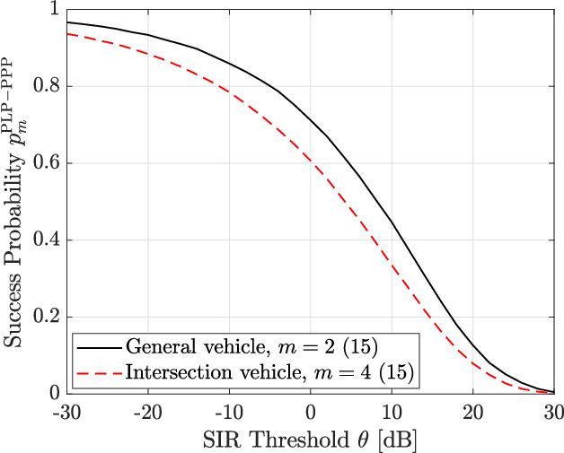
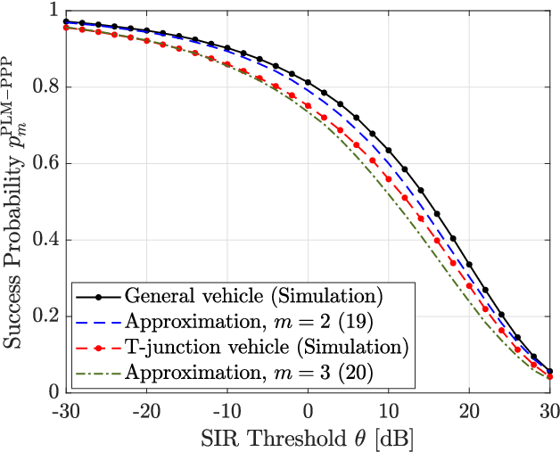
Fig. 5 compares the success probabilities of the typical general and intersection/T-junction vehicles. We omit the plot for the success probability of the typical vehicle in the OG-PPP as it is the same as that in the PLP-PPP by Proposition 1. We see that the success probability of the typical general vehicle is higher than that of the typical intersection/T-junction vehicle in all the Cox vehicular networks. The reason is that as two streets pass through or end at the typical vehicle at an intersection or a T-junction, the received interference is higher compared to the typical general vehicle through which only one street passes.
Remark 1.
Fig. 5c indicates that the success probability of the typical general vehicle in the PLM-PPP is tightly lower bounded by that in the PSP-PPP with Rayleigh distributed half-lengths.
Remark 2.
The approximation (20) to the success probability of the typical T-junction vehicle serves as a tight lower bound (see Fig. 5c). The integral term on the right-hand side of (20) is the Laplace transform of the interference from the vehicles on the street that has its endpoint at the origin. We can rephrase (20) as follows. The success probability of the typical T-junction vehicle in the PLM-PPP is tightly lower bounded by the success probability of the typical vehicle (with one street passing through) in the network formed by conditioning a street in the PSP-PPP (with Rayleigh distributed half-lengths) such that one of its endpoints is at the origin.
Next, we analyze the equivalence between the spatial models using their properties and the success probabilities of the typical vehicle in those models.
V Equivalence of Spatial Models
To differentiate the street intensities of the models OG, PLP, PSP, and PLM, we denote them as , , , and , respectively.
V-A OG-PPP and PLP-PPP
Theorem 2.
The PLP-PPP of street intensity is strictly equivalent to the OG-PPP with street intensity .
Proof:
The equivalence is a direct consequence of the success probabilities of the typical vehicle in the OG-PPP and PLP-PPP given in Proposition 1. ∎
V-B PSP-PPP and PLP-PPP
Theorem 3.
Let , where is a constant and is a random variable with mean 1. The PLP is the limiting process of the PSP as and such that .
Proof:

We formalize the heuristic arguments on the relation between the PLP and PSP given in [18]. From Definitions 4 and 5, we learn that the parameter spaces of line and stick are different. To compare the line process with the stick process, we first establish compatible parametrizations. Let denote the infinitely extended stick , where is the distance between the midpoint of the stick and , the closest point to the origin from . Fig. 6 illustrates and using overlaid dashed and solid lines, respectively. We can express and in terms of and as . The differential element equals , i.e., the alternate parametrizations are equivalent.
By (4), the line is just the projection of the stick from the parameter space to when the latter is extended to infinity. However, we learn from Lemmas 1 and 2 that the properties of the PLP and PSP differ. Then, to obtain the PLP from PSP, we need to equate their statistical properties. Equating the mean total street length per unit area in the PLP and PSP given in Lemmas 1 and 2, we obtain . For to remain finite, should go to zero as . ∎
Corollary 1.
The PSP-PPP, and its limiting case, the PLP-PPP, are strictly equivalent. As the PLP and PSP are identically distributed as and , equivalence is not restricted to PPPs on the streets but also holds for general point processes of vehicles.
V-C PLM-PPP and PSP-PPP
We learned from Proposition 4 that the success probability of the typical general vehicle in the PLM-PPP is approximated by that in the PSP-PPP with the same half-length density function as the PLM-PPP. Furthermore, from Figs. 4a and 4b, we infer that the th-nearest-neighbor distance distribution in the PLM-PPP is tightly upper bounded by that in the PSP-PPP. Consequently, we can deduce that the approximation to the success probability in the PLM-PPP is tight. Fig. 7 compares the simulated success probability of the typical general vehicle in the PLM-PPP with its lower bound. The maximum difference between the success probabilities in the PSP-PPP and PLM-PPP is for and 0.0219 for . Though the PLM can characterize T-junctions, it is too complex to permit an exact analytical expression.

Remark 3.
The PLM-PPP is equivalent with to the PSP-PPP with the same half-length distribution and street intensity as the PLM-PPP. Consequently, the PSP-PPP serves as a good substitute for the PLM-PPP.
We see from Fig. 7 that the success probabilities of the typical general vehicle in the PLM-PPP and PSP-PPP with Rayleigh distributed half-lengths are even closer in the asymptotic regions of than in the middle regions of . Theorem 4 proves this observation formally.
Theorem 4.
The PLM-PPP is asymptotically equivalent in both the lower and upper regimes of to the PSP-PPP with the same half-length density as the PLM-PPP.
Proof:
First, we study the asymptotic behavior of the PSP-PPP as and . Then, we compare them with that of the PLM-PPP.
Lemma 8.
As , the PSP-PPP behaves like a vehicular point process formed only by the typical vehicle’s streets, i.e.,
| (21) |
Proof:
See Appendix -I. ∎
Lemma 9.
As , the success probability of the typical vehicle in the PSP-PPP tends to that in a 2D PPP, i.e.,
| (22) |
where is the 2D intensity of the PSP-PPP.
Proof:
See Appendix -J. ∎
Equipped with the two lemmas, we continue with the proof of the theorem. As , for SIR to hold, it suffices not to have any interferers within a small disk around the typical vehicle. With high probability, the small disk intersects only the street(s) passing through the typical vehicle. Consequently, the system performance converges to that of only the typical vehicle’s streets as . The outage probability of the typical vehicle due to its streets alone is proportional to as . On the other hand, as , for SIR , a large disk around the typical vehicle must be devoid of interferers. It follows from Lemma 9 that the street geometry outside a large disk does not matter as since the PSP-PPP is similar to a 2D PPP at a large scale.
Lemma 8 extends to the PLM-PPP as the interaction between the sticks is irrelevant when . Also, the success probability of the typical general vehicle with respect to its street alone in the PLM-PPP is the same as that in the PSP-PPP with the same half-length density as the PLM-PPP. In Appendix -J, we reasoned that the PSP-PPP behaves like a 2D PPP as through mapping all the points on the sticks to their respective midpoints. The same logic holds for the PLM-PPP as it is also formed by sticks whose midpoints form a PPP. As the PLM-PPP and PSP-PPP with the same half-length density as the PLM-PPP behave like 2D PPPs of the same intensities as , they are equivalent as . ∎


| Model A | Model B | Conditions for Equivalence |
|---|---|---|
| OG-PPP | PLP-PPP | |
| PLP-PPP | PSP-PPP | and s.t. |
| PSP-PPP | PLM-PPP | , |
Fig. 8 compares the success probabilities of the typical general vehicle in the street-based Cox vehicular networks with that of the typical vehicle in 1D and 2D PPPs. The success probability of the typical vehicle in the PSP-PPP and PLM-PPP tends to that in the network formed only by the typical vehicle’s street(s) as and to that of the 2D PPP as , as given in Theorem 4 and the lemmas therein. The same holds for the PLP-PPP, as established in [20, Th. 4 and 5]. As vehicles on each street in the PLP-PPP form a 1D PPP, the PLP-PPP behaves like a 1D PPP as .
Until now, we have assumed that the link distance is fixed. Next, we discuss the equivalence between the spatial models when the link distances are random. Here, the success probability is obtained by averaging the Laplace transform of the interference over the link distances.
V-D Equivalence Under Random Link Distances
V-D1 PLP-PPP vs. OG-PPP
The OG-PPP is just a rotational variant of the PLP-PPP. Both of them have the same statistical properties such as the mean total street length per unit area (Lemma 1), distribution of the distance to the nearest-neighbor (Lemma 6), and the Laplace transform of the interference (Proposition 1). Hence, the OG-PPP and PLP-PPP are strictly equivalent even if the link distances are random.
V-D2 PSP-PPP vs. PLP-PPP
The PLP is the limiting process of the PSP as the lengths of the sticks extend to infinity and street intensity tends to zero (Theorem 3). By the inherent nature of the PSP, it is equivalent to the PLP irrespective of the mode of communication.
V-D3 PLM-PPP vs. PSP-PPP
We deduced from Figs. 4a and 4b that the th-nearest-neighbor (or interferer) distance distribution in the PLM-PPP is tightly upper bounded by that in the PSP-PPP with Rayleigh distributed half-lengths. It follows that irrespective of the distribution of the distance to the intended transmitter, the PLM-PPP and PSP-PPP with Rayleigh distributed half-lengths are equivalent. Fig. 9 validates the above inference for the case where the typical general vehicle receives a message from its nearest neighbor (transmitter) through simulations.

Remark 4.
The notion of equivalence enables us to consider only a representative set of spatial models to obtain insights on the effect of the network parameters, thereby reducing the computational costs and time associated with large-scale experiments and system-level simulations. The success probabilities of the typical vehicle in the OG-PPP, PLP-PPP, and PLM-PPP can be obtained from that in the PSP-PPP by a suitable mapping between the parameters as summarized in Table I.
VI Conclusions and Future Work
We developed a Coxian framework for the modeling and analysis of vehicular networks. The spatial models in this framework can characterize different street geometries involving intersections and T-junctions, and street lengths that can be independent or dependent on each other. Streets of infinite lengths and different orientations forming intersections can be characterized by PLPs and their rotational variants. PSPs and PLMs can model streets of varying finite lengths forming intersections and T-junctions, respectively. We evaluated the reliability of a vehicle-to-vehicle link in the Cox vehicular networks when the receiving vehicle is at an intersection, a T-junction, or a general location, and its transmitter is at a certain fixed distance. Our approach to defining the street system as a union of points of different orders facilitates general analytical results for different types of typical vehicles. The expressions for the reliability can be used to investigate the interplay among the network parameters such as data rate, street intensity, vehicle density, and the type of vehicle.
The concept of equivalence demonstrates that one does not need different spatial models to analyze the reliability of a vehicle-to-vehicle link in different geographical regions. The models considered in the Coxian framework are equivalent in terms of reliability. This implies that the expression for the reliability of the typical vehicle in the PSP-PPP is sufficient to evaluate that in the OG-PPP, PLP-PPP, and PLM-PPP by appropriately mapping the system parameters. Also, the vehicular networks behave like PPPs only in the asymptotic regimes of the reliability or data rate. Hence, the street geometry is relevant to understand vehicular network behavior.
An interesting future extension would be to understand how two or more models developed in the Coxian framework can be superimposed to represent an intricate geographic region with intersections and T-junctions, and streets and highways. Also, one may look for tractable models that characterize curved streets and examine whether they are equivalent to the line/stick-based vehicular networks.
-A Proof of Lemma 4
To prove Lemma 4, we make use of [17, Prop. 6.2], which asserts the following: There exist , such that the complementary cumulative distribution function (CCDF) of the half-lengths in the lilypond model can be bounded as
| (23) |
Our goal is to find a tight approximation. By the properties of the cumulative distribution function, . However, makes the bound (23) loose for small , which implies that is the natural choice. This reduces the bound (23) to the CCDF of the Rayleigh distribution. Fig. 10 fits the CCDF and PDF of the half-lengths to that of the Rayleigh distribution. We observe that the upper bound on the CCDF is loose for small values of . Instead of choosing a value for that provides an upper bound, we approximate the CCDF of the half-lengths with an appropriate value for that minimizes the gap between the empirical and theoretical CCDFs. It follows from the Rayleigh approximation that the mean half-length is . The value of is found by equating to the empirical mean of the half-lengths.


Next, we study the relation between and . Suppose we scale the PLM by an arbitrary factor . Then the street intensity is scaled by and the half-lengths of the sticks are scaled by , inversely proportional to . As the PLM retains its lilypond nature with scaling, the mean of the scaled half-lengths is scale-invariant, i.e., . This implies that , and thus scales with .
| (27) | ||||
| (28) |
-B Proof of Lemma 5
For the typical vehicle at the origin, the probability that its nearest neighbor is at a distance greater than , , is given by
| (24) |
where and exploit the independence of the 1D PPPs.
The contact distance distribution is the probability of finding a vehicle within a distance from an arbitrary location in the plane, say the origin. No streets pass through or contain the origin a.s. This implies that is defined with respect to , which is equivalent in distribution to . Hence .
-C Proof of Lemma 6
Using the probability generating functional (PGFL) of the PPP, we can express in (24) as
| (25) |
where follows from the independence between and and the fact that for the OG-PPP/PLP-PPP. Since the vehicle locations follow a 1D PPP, with respect to the streets that pass through the origin, we have .
-D Proof of Theorem 1
The probability that there are no vehicles on a stick within a distance from the origin is . We derive as follows: The midpoint is denoted as in polar coordinates. Using (5), we can express the points on a stick of length as , . Then the squared distance between a point on and the origin is . The points of intersection of on are at distances from the midpoint of the stick. They follow from solving
| (26) |
with respect to . For a stick to intersect , must be within . We consider two cases—, and :

1. : Let for . When
- a.
: The stick lies within . Then .
- b.
: The stick is not fully contained in . For a stick that passes through , . For a stick with only one endpoint in , or .
Summarizing the above cases, we write .
2. : Let for . When
- a.
: The stick does not intersect . Then .
- b.
: For a stick that passes through , . For a stick with only one endpoint in , or .
Thus, . Then the probability of not finding a vehicle on within is , where . Fig. 11 illustrates the above cases.
For the typical vehicle’s street to pass through or end at the origin, its midpoint must belong to . The midpoint of the typical vehicle’s street of half-length is at a distance from the origin. Using the above results and the decomposition of the nearest-neighbor distance distribution in Lemma 5, we can write and as in (27) and (28), respectively, by applying the PGFL of the PPP.
-E Proof of Proposition 1
By (4), we can express the points on as , . Let refer to the th-nearest point in from the origin. Then denotes the point process of vehicles on (Section II-E). The Laplace transform of the interference from the vehicles on to the typical vehicle at the origin is given by
| (29) | ||||
| (30) |
where , substitutes and the PGFL of the PPP. is the intensity of the active transmitters for which , . is due to the change of variable , and .
We learned from (14) that the success probability is the product of the Laplace transforms of the interference and , which we derive below.
| (41) | ||||
| (42) | ||||
| (43) | ||||
| (44) |
-E1 Laplace Transform of
The Laplace transform of the interference from to the typical general vehicle (order 2) can be obtained by setting in (30), i.e.,
| (31) |
For the typical intersection vehicle (order 4), as two streets pass through the origin, (Sec. II-E). Then can be written as in (29) as follows:
| (32) |
where results from being identically distributed as . It follows that .
-E2 Laplace Transform of
The aggregate Laplace transform of the interference from the vehicles on all the streets that do not pass through the typical vehicle is given by
| (33) | ||||
| (34) |
where follows from and the fact that the ’s are independent 1D PPPs, uses (30) and the PGFL of the PPP with respect to and , and results from being independent of , and . Substituting (31), (32), and (34) in (14), we obtain (15).
-F Proof of Proposition 2
Using (5), we can denote the points on a stick of length as , . The midpoint of the street that passes through the typical vehicle is at a signed distance from the origin. Then the endpoints of the street are at signed distances , and to the origin. As in (29), the Laplace transform of the interference for the typical general vehicle can be written as
| (35) | ||||
| (36) |
where substitutes and applies the PGFL of the PPP, and results from the change of variable . evaluates the expectation with respect to using rather than based on Lemma 3. For the typical intersection vehicle, as two streets pass through the origin and the point processes on them are independent, the corresponding Laplace transform of the interference is the square of that given in (36) similar to (32).
-G Proof of Proposition 3
This proof uses the same notation as in Appendix -F. Let and . From Section II-E, we have , , denoting the point process of vehicles on the th street that does not pass through the origin. The Laplace transform of the interference from the vehicles on is
| (37) |
where applies the PGFL of the PPP, , and .
-H Proof of Proposition 4
-H1 Success probability of the typical general vehicle in the PLM-PPP
We learned from Conjecture 1 that the probability of finding the th-nearest neighbor closer is higher in the PSP-PPP than in the PLM-PPP. Consequently, the success probability of the typical general vehicle in the PLM-PPP is lower bounded by that in the PSP-PPP. As this inference is based on a conjecture, we present the result for the success probability of the typical general vehicle in the PLM-PPP as an approximation rather than a bound. By (12) and (14), we have
| (39) |
-H2 Success probability of the typical T-junction vehicle in the PLM-PPP
We have , where denote the vehicles on the street that passes through the origin, and denote the vehicles on the street with one endpoint at the T-junction. The success probability of the typical T-junction vehicle (order 3), , is given by
| (40) |
where assumes independence between and , and follows from (39). The integral expression in can be derived similarly to (36) using the detail that for the street whose one endpoint is a T-junction at the origin, its other endpoint is at a distance from the origin. is the approximated density of the half-length of the street that ends at a T-junction.
-I Proof of Lemma 8
We can approximate given by (38) using Taylor’s series as as in (41). Using (35) and (41), the outage probability as , can be written as in (42), where . By interchanging the limit and expectation (using the monotone convergence theorem), and applying Taylor’s theorem inside the expectation in (42), we obtain (43). It transforms to (44) by the change of variable , whose integral term evaluates to a constant as . Note that depends on .
-J Proof of Lemma 9
Consider a model formed by mapping all the points on each stick to its midpoint. The expected number of active transmitters on each stick is . Since the midpoints follow a 2D PPP of intensity , forms a non-simple 2D PPP with density . It can be seen as a marked point process whose ground process is a 2D PPP of intensity and the marks refer to the multiplicity of the points. Let define the mapping from to . Using (6) and (7), the success probability of the typical vehicle in the PSP-PPP can be expressed as
Similarly, the success probability of the typical vehicle in is written as
For sticks of half-length , . Then
| (45) |
Then as . The order of the typical vehicle is irrelevant as the mapping does not distinguish an intersection from a non-intersection. The success probability of the typical vehicle can be obtained by substituting in (11).
References
- [1] Q. Cui, N. Wang, and M. Haenggi, “Vehicle distributions in large and small cities: Spatial models and applications,” IEEE Transactions on Vehicular Technology, vol. 67, no. 11, pp. 10 176–10 189, Nov. 2018.
- [2] C. Jiang, H. Zhang, Z. Han, Y. Ren, V. C. M. Leung, and L. Hanzo, “Information-sharing outage-probability analysis of vehicular networks,” IEEE Transactions on Vehicular Technology, vol. 65, no. 12, pp. 9479–9492, Dec. 2016.
- [3] Y. Jeong, J. W. Chong, H. Shin, and M. Z. Win, “Intervehicle communication: Cox-Fox modeling,” IEEE Journal on Selected Areas in Communications, vol. 31, no. 9, pp. 418–433, Sep. 2013.
- [4] B. Błaszczyszyn, P. Mühlethaler, and Y. Toor, “Stochastic analysis of ALOHA in vehicular ad hoc networks,” Annals of Telecommunications, vol. 68, no. 1, pp. 95–106, 2013.
- [5] K. Koufos and C. P. Dettmann, “The meta distribution of the SIR in linear motorway VANETs,” IEEE Transactions on Communications, vol. 67, no. 12, pp. 8696–8706, Dec. 2019.
- [6] E. Steinmetz, M. Wildemeersch, T. Q. S. Quek, and H. Wymeersch, “A stochastic geometry model for vehicular communication near intersections,” in 2015 IEEE Globecom Workshops, San Diego, CA, USA, Dec. 2015, pp. 1–6.
- [7] P. Crucitti, V. Latora, and S. Porta, “Centrality in networks of urban streets,” Chaos: An Interdisciplinary Journal of Nonlinear Science, vol. 16, no. 1, pp. 0 151 131–0 151 139, 2006.
- [8] V. V. Chetlur and H. S. Dhillon, “Coverage analysis of a vehicular network modeled as Cox process driven by Poisson line process,” IEEE Transactions on Wireless Communications, vol. 17, no. 7, pp. 4401–4416, Jul. 2018.
- [9] F. Morlot, “A population model based on a Poisson line tessellation,” in 2012 International Symposium on Modeling and Optimization in Mobile, Ad Hoc and Wireless Networks (WiOpt), May 2012, pp. 337–342.
- [10] C. Choi and F. Baccelli, “An analytical framework for coverage in cellular networks leveraging vehicles,” IEEE Transactions on Communications, vol. 66, no. 10, pp. 4950–4964, Oct. 2018.
- [11] V. V. Chetlur and H. S. Dhillon, “Coverage and rate analysis of downlink cellular vehicle-to-everything (C-V2X) communication,” IEEE Transactions on Wireless Communications, vol. 19, no. 3, pp. 1738–1753, Mar. 2020.
- [12] V. V. Chetlur and H. S. Dhillon, “Success probability and area spectral efficiency of a VANET modeled as a Cox process,” IEEE Wireless Communications Letters, vol. 7, no. 5, pp. 856–859, Oct. 2018.
- [13] C. Choi and F. Baccelli, “Poisson Cox point processes for vehicular networks,” IEEE Transactions on Vehicular Technology, vol. 67, no. 10, pp. 10 160–10 165, Oct. 2018.
- [14] M. N. Sial, Y. Deng, J. Ahmed, A. Nallanathan, and M. Dohler, “Stochastic geometry modeling of cellular V2X communication over shared channels,” IEEE Transactions on Vehicular Technology, vol. 68, no. 12, pp. 11 873–11 887, Dec. 2019.
- [15] F. Voss, C. Gloaguen, F. Fleischer, and V. Schmidt, “Distributional properties of Euclidean distances in wireless networks involving road systems,” IEEE Journal on Selected Areas in Communications, vol. 27, no. 7, pp. 1047–1055, Sep. 2009.
- [16] M. Haenggi, Stochastic Geometry for Wireless Networks. Cambridge University Press, 2012.
- [17] D. J. Daley, S. Ebert, and G. Last, “Two lilypond systems of finite line-segments,” Probability and Mathematical Statistics, vol. 36, no. 2, pp. 221–246, 2016.
- [18] P. Parker and R. Cowan, “Some properties of line segment processes,” Journal of Applied Probability, vol. 13, no. 1, pp. 96–107, 1976.
- [19] W. E. Stein and R. Dattero, “Sampling bias and the inspection paradox,” Mathematics Magazine, vol. 58, no. 2, pp. 96–99, 1985.
- [20] J. P. Jeyaraj and M. Haenggi, “A transdimensional Poisson model for vehicular networks,” in 2019 IEEE Global Communications Conference (GLOBECOM), Hawaii, USA, Dec. 2019.
![[Uncaptioned image]](2106.06836v1/Jeya.jpg) |
Jeya Pradha Jeyaraj (S’17) received the M.Tech degree in electrical engineering from the Indian Institute of Technology Kanpur, India, in 2013. She is currently pursuing the Ph.D. degree in electrical engineering at the University of Notre Dame, Indiana, USA, since 2016. She is also working towards the M.S. degree in applied and computational mathematics and statistics. Before joining her Ph.D., she worked as a Software Development Engineer in the 3G cellular technologies group at Cisco Systems, India. She held internship positions in the research and development divisions at Toyota Motor North America and Qualcomm in the USA. Her research interests include vehicular networks, stochastic geometry, spectrum sharing, and data mining. |
![[Uncaptioned image]](2106.06836v1/Haenggi.jpg) |
Martin Haenggi (S‘95-M‘99-SM‘04-F‘14) received the Dipl.-Ing. (M.Sc.) and Dr.sc.techn. (Ph.D.) degrees in electrical engineering from the Swiss Federal Institute of Technology in Zurich (ETH) in 1995 and 1999, respectively. Currently he is the Freimann Professor of Electrical Engineering and a Concurrent Professor of Applied and Computational Mathematics and Statistics at the University of Notre Dame, Indiana, USA. In 2007-2008, he was a visiting professor at the University of California at San Diego, and in 2014-2015 he was an Invited Professor at EPFL, Switzerland. He is a co-author of the monographs "Interference in Large Wireless Networks" (NOW Publishers, 2009) and ‘Stochastic Geometry Analysis of Cellular Networks’ (Cambridge University Press, 2018) and the author of the textbook "Stochastic Geometry for Wireless Networks" (Cambridge, 2012), and he published 16 single-author journal articles. His scientific interests lie in networking and wireless communications, with an emphasis on cellular, amorphous, ad hoc (including D2D and M2M), cognitive, and vehicular networks. He served as an Associate Editor of the Elsevier Journal of Ad Hoc Networks, the IEEE Transactions on Mobile Computing (TMC), the ACM Transactions on Sensor Networks, as a Guest Editor for the IEEE Journal on Selected Areas in Communications, the IEEE Transactions on Vehicular Technology, and the EURASIP Journal on Wireless Communications and Networking, as a Steering Committee member of the TMC, and as the Chair of the Executive Editorial Committee of the IEEE Transactions on Wireless Communications (TWC). From 2017 to 2018, he was the Editor-in-Chief of the TWC. Currently he is an editor for MDPI Information. For both his M.Sc. and Ph.D. theses, he was awarded the ETH medal. He also received a CAREER award from the U.S. National Science Foundation in 2005 and three awards from the IEEE Communications Society, the 2010 Best Tutorial Paper award, the 2017 Stephen O. Rice Prize paper award, and the 2017 Best Survey paper award, and he is a Clarivate Analytics Highly Cited Researcher. |