On a parabolic sine-Gordon model

Xinyu Cheng Address: X.Y. Cheng, Department of Mathematics, University of British Columbia, Vancouver, BC V6T 1Z2, Canada Email address: xycheng@math.ubc.ca , Dong Li Address: D. Li, Department of Mathematics, the Hong Kong University of Science & Technology, Clear Water Bay, Kowloon, Hong Kong Email address: mpdongli@gmail.com , Chaoyu Quan Address: C.Y. Quan, SUSTech International Center for Mathematics, Southern University of Science and Technology, Shenzhen, P.R. China Email address: quancy@sustech.edu.cn and Wen Yang Address: W. Yang, Wuhan Institute of Physics and Mathematics, Chinese Academy of Sciences, P.O. Box 71010, Wuhan 430071, P. R. China; Innovation Academy for Precision Measurement Science and Technology, Chinese Academy of Sciences, Wuhan 430071, P. R. China. Email address: wyang@wipm.ac.cn

Abstract.

We consider a parabolic sine-Gordon model with periodic boundary conditions. We prove a fundamental maximum principle which gives a priori uniform control of the solution. In the one-dimensional case we classify all bounded steady states and exhibit some explicit solutions. For the numerical discretization we employ first order IMEX, and second order BDF2 discretization without any additional stabilization term. We rigorously prove the energy stability of the numerical schemes under nearly sharp and quite mild time step constraints. We demonstrate the striking similarity of the parabolic sine-Gordon model with the standard Allen-Cahn equations with double well potentials.

1. Introduction

In this work we are concerned with the following parabolic sine-Gordon equation:

(1.1)

\begin{cases}\partial_{t}u=\kappa^{2}\Delta u+\sin u,\quad(t,x)\in(0,\infty)\times\Omega,\\ u\bigr|_{t=0}=u_{0},\end{cases}

where $\kappa^{2}$ is the diffusion constant and $\Omega$ is either a periodic torus $\mathbb{T}=[-\pi,\pi]$ in 1D or the torus $\mathbb{T}^{2}=[-\pi,\pi]\times[-\pi,\pi]$ in 2D. The unknown function $u:\;\Omega\to\mathbb{R}$ typically represents the concentration difference in the phase field context. For smooth solutions, the basic energy associated with (1.1) is

(1.2)

E(u)=\int_{\Omega}\left(\frac{\kappa^{2}}{2}|\nabla u|^{2}+\cos u\right)dx.

The fundamental energy conservation law takes the form

(1.3)

\frac{d}{dt}E(u)+\int_{\Omega}|\partial_{t}u|^{2}dx=0.

It follows that

(1.4)

E(u(t))\leq E(u(s)),\quad\forall\,t\geq s,

which gives a priori control of the homogeneous $\dot{H}^{1}$ -norm of the solution. Better estimates are also available. For example assuming $u_{0}$ is bounded, then by using the fact that the nonlinear term $\sin u$ is bounded by 1, one can show that the solution remains bounded for all finite time. Bootstrapping from this then easily yields global wellposedness and regularity of the solution. Somewhat akin to the equation (1.1) is the following slightly more general model

(1.5)

\displaystyle\partial_{\tau}v=\kappa^{2}\Delta v+\gamma\sin\beta v,

where $\beta>0$ , $\gamma>0$ are parameters, and we denote by $\tau$ the time variable. One can rewrite (1.5) as

(1.6)

\displaystyle\frac{\partial(\beta v)}{\partial(\gamma\beta\tau)}=\frac{\kappa^{2}}{\gamma\beta}\Delta(\beta v)+\sin(\beta v).

Consequently a change of variable $u=\beta v$ , $t=\gamma\beta\tau$ transforms (1.5) into the standard form (1.1).

The classical one dimensional sine-Gordon equation

(1.7)

\displaystyle\partial_{tt}\phi-\partial_{xx}\phi=-\sin\phi

dates back at least to Frenkel and Kontorova [8] who considered the motion of a slip in an infinite chain of atoms lying on top of a given fixed chain of alike atoms. To study the propagation of the slip they obtained a difference differential equations which was approximated by the sine-Gordon equation (1.7). In the realm of nonlinear field theory, the sine-Gordon equation

(1.8)

\displaystyle\partial_{tt}\phi-\partial_{xx}\phi=-m^{2}\sin\phi

arises as one of the simplest intrinsically nonlinear theories. The classical point-like particle theories suffer divergence problems such as the well-known self-energy problem of electrodynamics. It was realized that (cf. the discussion on pp. 260 of [1]) one must consider nonlinear field theory in order to predict both the existence and dynamics of extended elementary particles. Instead of augmenting a linear theory with the addition of a nonlinear term ad hoc, a more natural way is to postulate a field whose target is a nonlinear manifold. In this context the simplest topologically nontrivial manifold is the standard $1$ -sphere, i.e. the set of real numbers modulo $2\pi$ . The sine-Gordon Lagrangian density is postulated as

(1.9)

\displaystyle\mathcal{L}_{\mathrm{S}G}=\frac{1}{2}\bigl(\phi_{t}^{2}-\phi_{x}^{2}-2m^{2}(1-\cos\phi)\bigr).

One should note that for small $\phi$ , we have $2m^{2}(1-\cos\phi)\approx m^{2}\phi^{2}$ , i.e. we can recover the usual Klein-Gordon Lagrangian density

(1.10)

\displaystyle\mathcal{L}_{\mathrm{KG}}=\frac{1}{2}\bigl(\phi_{t}^{2}-\phi_{x}^{2}-m^{2}\phi^{2}).

The significance of the term $2m^{2}(1-\cos\phi)$ is that it is the simplest periodic function of $\phi$ which coincides with the Klein-Gordon case in the low-amplitude limit. The periodicity of the nonlinear term has the effect of restricting the range of $\phi$ to be the $1$ -sphere. Already within the limits of one-dimensional classical field theory, the sine-Gordon equation (1.8) gave a very good picture of the interaction of elementary particles and the existence of bound states, and in particular it may lead to to solutions with the collisional properties of solitons [14, 16]. The sine-Gordon equation has also been studied as a model in the theory of crystal dislocations, the motion of rigid pendular attached to stretched wire, and splay waves in lipid membranes and magnetic flux on Josephson line. We refer the interested readers to [1, 2, 3, 6, 7, 8, 10, 13, 15] and the references therein for more extensive discussions.

Refer to caption — Figure 1. Comparison of the double-well potentials $F(u)$ between the sine-Gordon model and the Allen-Cahn model with polynomial potential.

Our parabolic sine-Gordon model (1.1) can be viewed as the parabolic version of the usual wave-type sine-Gordon in the phase-field context. It naturally arises from the gradient flow of the energy functional

(1.11)

\displaystyle\mathcal{E}_{\mathrm{SG}}(u)=\int_{\Omega}\left(\frac{\kappa^{2}}{2}|\nabla u|^{2}+\cos u\right)dx

in $L^{2}(\Omega)$ . Note that if we consider the $H^{-1}$ -gradient flow of (1.11), then we obtain the model:

(1.12)

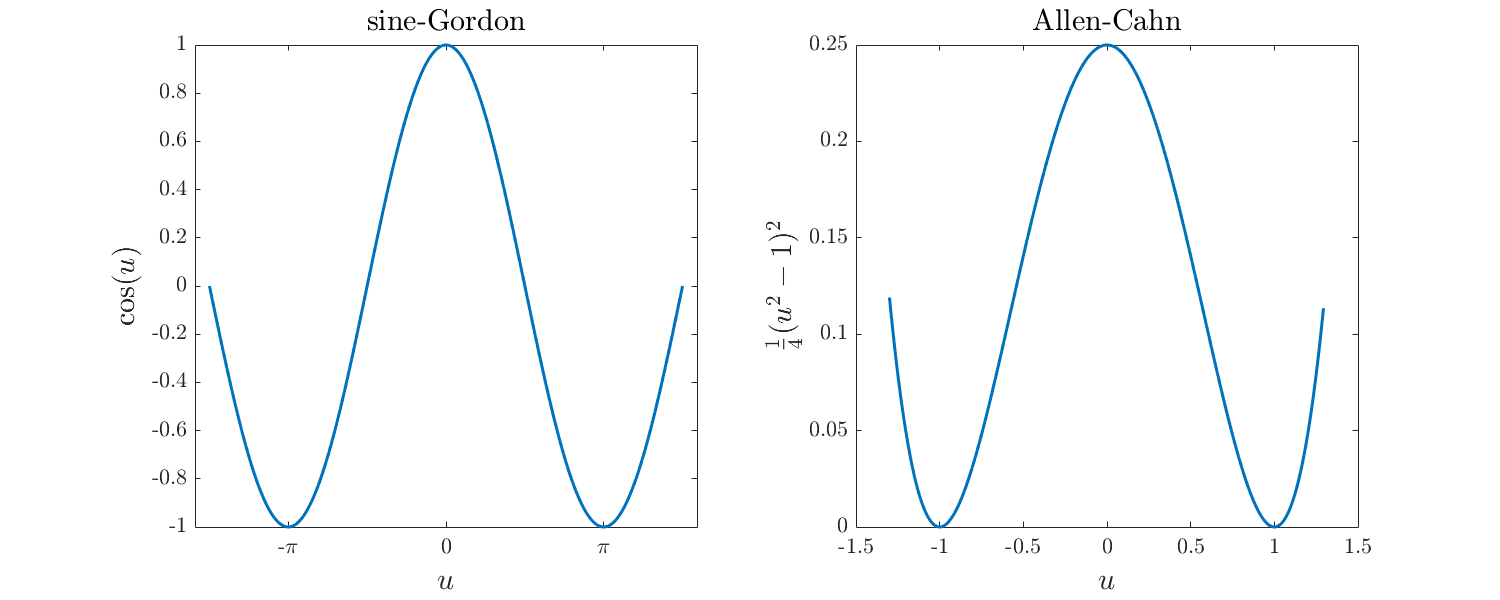
\displaystyle\partial_{t}u=\Delta(-\kappa^{2}\Delta u-\sin u)

which is akin to the usual Cahn-Hilliard equation. The model (1.12) will be studied elsewhere. As it turns out, the potential term $F_{\mathrm{SG}}(u)=\cos u$ looks qualitatively similar to the usual double well potential $F_{\mathrm{st}}(u)=(u^{2}-1)^{2}/4$ for $|u|=O(1)$ , cf. Figure 1. For this reason it is natural to speculate that there is some natural one-to-one correspondence between solutions to the parabolic sine-Gordon equation (1.1) and the usual Allen-Cahn equations. On the other hand, the parabolic sine-Gordon equation is quite appealing for both analysis and simulation since its nonlinearity has bounded derivatives of all orders. As a matter of fact, the potential $F_{\mathrm{SG}}(u)=\cos u$ is one of the handy choices for testing and benchmarking algorithms in the computational phase field community. The purpose of this work is to initiate the study of (1.1) and establish a number of basic facts for solutions to (1.1). More importantly we prove the fundamental monotonicity laws for the solutions, characterize and classify one-dimensional steady states, and analyze the stability of several prototypical numerical discretization schemes implemented on this model. Remarkably due to the very benign nonlinear structure one can prove optimal energy stability results without resorting to any $L^{\infty}$ -maximum principle. This feature is quite appealing and we expect future development of our analysis on the model (1.12) under slightly more stringent time step constraints.

The rest of this paper is organized as follows. In Section 2 we prove a fundamental maximum principle of the parabolic sine-Gordon model in all dimensions. In Section 3 we classify all bounded steady state solutions in one dimension. In Section 4 we analyze two numerical discretization schemes and prove optimal energy stability. In Section 5 we carry out several numerical experiments showcasing the striking similarity of the parabolic sine-Gordon model and the usual Allen-Cahn equation. In the last section we give concluding remarks.

2. Maximum principle

In this section we prove a useful maximum principle for (1.1) on the the torus $\mathbb{T}^{d}=[-\pi,\pi]^{d}$ for all dimensions $d\geq 1$ .

Theorem 2.1 (Globalwell posedness and maximum principle).

Let $\kappa>0$ and consider (1.1) on $\mathbb{T}^{d}=[-\pi,\pi]^{d}$ , $d\geq 1$ . Suppose $\|u_{0}\|_{\infty}\leq\pi$ . Then there exists a unique global solution $u$ to (1.1) which is smooth for all $t>0$ . Furthermore we have

(2.1)

\displaystyle\sup_{0\leq t<\infty}\|u(t,\cdot)\|_{\infty}\leq\pi.

Proof.

We begin by noting that since the nonlinear term $\sin u$ has uniformly bounded derivatives of all orders, it is utterly standard to obtain the global wellposedness and regularity of the solution to (1.1) and thus we focus on the proof of (2.1).

We first prove (2.1) under the assumption that $\|u_{0}\|_{\infty}<\pi$ . Since $\|u_{0}\|_{\infty}<\pi$ , by using smoothing estimate we may assume with no loss that $u_{0}$ is smooth and still satisfy $\|u_{0}\|_{\infty}<\pi$ . Fix $0<\varepsilon\ll 1$ which will be taken to tend to zero later and consider $v(t,x)=u(t,x)-\pi-\varepsilon$ . We claim the following:

(2.2)

\displaystyle\sup_{t\geq 0}\max_{x\in\mathbb{T}^{d}}v(t,x)\leq 0.

Assume the claim is not true, then we can find $t_{*}>0$ such that

(2.3)			$\displaystyle\max_{x\in\mathbb{T}^{d}}v(t_{*},x)=0,$
(2.4)			$\displaystyle\max_{x\in\mathbb{T}^{d}}v(t,x)>0,\qquad t\in(t_{},t_{}+\delta_{0}),$

where $\delta_{0}>0$ is a sufficiently small constant. Assume $v(t_{*},x)$ takes its maximum at some $x_{*}\in\mathbb{T}^{d}$ . Note that $u(t_{*},x_{*})=\pi+\varepsilon$ . We have

(2.5)

\displaystyle\partial_{t}v(t,x_{*})\Bigr|_{t=t_{*}}\leq\sin(\pi+\varepsilon)=-\sin\varepsilon<0.

By continuity, we can find $\delta_{*}>0$ sufficiently small such that if $|t-t_{*}|+|y-x_{*}|<3\delta_{*}$ , then

(2.6)

\displaystyle\partial_{t}v(t,y)<-\frac{1}{2}\sin\varepsilon<0.

In particular, for $|y-x_{*}|<\delta_{*}$ and $|t-t_{*}|<\delta_{*}$ , we have

(2.7)

\displaystyle v(t,y)\leq 0.

Now for $t=t_{*}$ and any $x\in\mathbb{T}^{d}$ such that $v(t,x)<0$ , we can find a neighborhood $N_{x}$ and $\delta_{x}>0$ such that for any $t\in[t_{*},t_{*}+\delta_{x}]$ , $y\in N_{x}$ ,

(2.8)

\displaystyle v(t,y)<0.

By a covering argument using (2.7) and (2.8) (if $v(t_{*},x)=0$ we use (2.7), and if $v(t_{*},x)<0$ we use (2.8)), we obtain for $t_{*}\leq t\leq t_{*}+\delta_{1}$ and $\delta_{1}>0$ sufficiently small,

(2.9)

\displaystyle\max_{t_{*}\leq t\leq t_{*}+\delta_{1}}\max_{x\in\mathbb{T}^{d}}v(t,x)\leq 0.

This clearly contradicts (2.4) and thus the claim (2.2) holds.

By taking $\varepsilon\to 0$ , we obtain $u(t,x)\leq\pi$ for all $x\in\mathbb{T}^{d}$ and $t\geq 0$ . By working with $-u$ we obtain $u(t,x)\geq-\pi$ for all $x\in\mathbb{T}^{d}$ and $t\geq 0$ . The desired result then follows easily.

Finally we show how to get (2.1) under the assumption that $\|u_{0}\|_{\infty}\leq\pi$ . It suffices for us to show for any finite $T>0$ ,

(2.10)

\displaystyle\sup_{0\leq t\leq T}\|u(t,\cdot)\|_{\infty}\leq\pi.

The trick is to use stability. For $n\geq 1$ , consider (1.1) with initial data $u_{0}^{(n)}=(1-2^{-n-1})u_{0}$ and denote the corresponding solution as $u^{(n)}$ . Apparently we have

(2.11)

\displaystyle\sup_{0\leq t\leq T}\|u^{(n)}(t,\cdot)\|_{\infty}\leq\pi,\quad\forall\,n\geq 1.

Observe that

(2.12)

\displaystyle u(t)-u^{(n)}(t)=e^{\kappa^{2}t\Delta}(u_{0}-u_{0}^{(n)})+\int_{0}^{t}e^{\kappa^{2}(t-s)\Delta}(\sin u(s)-\sin u^{(n)}(s))ds.

From this one can extract the $L^{\infty}$ -stability estimate of $u-u^{(n)}$ . In particular, it is not difficult to check that

(2.13)

\displaystyle\sup_{0\leq t\leq T}\|u(t,\cdot)-u^{(n)}(t,\cdot)\|_{\infty}\to 0,

as $n\to\infty$ . Thus (2.10) follows. ∎

3. Classification of the steady states in 1D

In this section we consider bounded steady states of the sine-Gordon equation,

(3.1)

\kappa^{2}u^{\prime\prime}+\sin u=0,\quad x\in\mathbb{R}.

Note that here we consider the whole real axis for generality. Functions on the torus $\mathbb{T}=[-\pi,\pi]$ can be naturally identified as a periodic function on $\mathbb{R}$ .

Proposition 3.1 (Rigidity of the solution to (3.1)).

The following hold.

•

Even reflection. Suppose $\kappa>0$ , and for some $r_{0}>0$ we have

(3.2) $\displaystyle\kappa^{2}u^{\prime\prime}+\sin u=0,\qquad\forall\,-r_{0}<x<0,$

where $u\in C^{2}((-r_{0},0))$ and we assume $\lim\limits_{x\to 0-}u^{\prime}(x)=0$ . Define $u(x)=u(-x)$ for $0<x<r_{0}$ . Then it holds that $u\in C^{\infty}((-r_{0},r_{0}))$ with $u^{\prime}(0)=0$ and solving the same equation on the whole interval.
•

Odd reflection. Suppose $\kappa>0$ , and for some $r_{0}>0$ we have

(3.3) $\displaystyle\kappa^{2}u^{\prime\prime}+\sin u=0,\qquad\forall\,0<x<r_{0}.$

where $u\in C^{2}((0,r_{0}))$ and we assume $\lim\limits_{x\to 0+}u(x)=0$ . Define $u(x)=-u(-x)$ for $-r_{0}<x<0$ . Then it holds that $u\in C^{\infty}((-r_{0},r_{0}))$ with $u(0)=0$ and solving the same equation on the whole interval.

Proof.

We shall only prove the first case as the second case is similar. First it is not difficult to that $u$ has bounded derivatives in $[-r_{0}/2,0)$ which can be extended to $0$ from the left. The extended $u$ satisfies the equation on $(-r_{0},0)\cap(0,r_{0})$ . Furthermore the equation also holds at $x=0$ up to third order derivatives. Then we can bootstrap the regularity of $u$ by using the equation and conclude that $u\in C^{\infty}$ . ∎

It is easy to see that if $u$ is a solution to (3.1), then for any integer $m\in\mathbb{Z}$ and $x_{0}\in\mathbb{R}$ , $u(\cdot+x_{0})+2m\pi$ is still a solution to (3.1). Therefore with no loss we can consider solutions $u$ with $|u(0)|\leq\pi.$

Multiplying (3.1) by $u^{\prime}$ , we derive

(3.4)

\frac{1}{2}\kappa^{2}(u^{\prime})^{2}=C+\cos u,

where $C\geq-1$ is a constant. Concerning the solution of (3.1), we have the following result.

Proposition 3.2.

Let $u$ be a bounded solution to (3.1) with $|u(0)|\leq\pi$ and $C\geq-1$ be the constant defined in (3.4), then the following hold.

(1)

For $C>1$ , there does not exist any bounded solution.
(2)

If $C=-1$ , then $u\equiv 0.$
(3)

If $C=1$ , then $u=\pm 2\arcsin\tanh\left(\frac{x}{\kappa}+c\right)$ for some constant $c\in\mathbb{R}$ or $u\equiv\pm\pi$ .
(4)

If $-1<C<1$ , then $u$ is a periodic function and $\|u\|_{\infty}<\pi$ .

Proof.

We proceed in several steps.

(1) If $C>1$ , then $u^{\prime}$ never changes its sign and it implies that $u$ is either an increasing or a decreasing function. In addition $|u^{\prime}|$ has a positive lower bound, it implies that $u$ is unbounded. Thus, there is no bounded solution for $C>1$ .

(2) If $C=-1$ , then

(3.5)

\cos u-1=\frac{1}{2}\kappa^{2}(u^{\prime})^{2}\geq 0,\quad\forall\,x\in\mathbb{R}.

Since $|u(0)|\leq\pi$ , it follows that $u\equiv 0$ .

(3) In the case $C=1$ , it is easy to check that $u\equiv\pi$ or $-\pi$ is always a solution. On the other hand when $|u(0)|<\pi$ , we can explicitly solve (3.4) and get

u=\pm 2\arcsin\tanh\left(\frac{x}{\kappa}+c\right),

where $c$ is a constant.

(4) In the case $C\in(-1,1)$ , note that $\arccos(-C)\in(0,\pi)$ . By (3.4) and the assumption that $|u(0)|\leq\pi$ , we have $|u(0)|\leq\arccos(-C)$ . We first discuss the case $|u(0)|<\arccos(-C)$ . In this case (3.4) simplifies to

(3.6)

\displaystyle u^{\prime}=\pm\frac{\sqrt{2}}{\kappa}\sqrt{C+\cos u}.

With no loss we consider the case $u^{\prime}(0)>0$ and work with the ODE:

(3.7)

\displaystyle u^{\prime}=\frac{\sqrt{2}}{\kappa}\sqrt{C+\cos u}.

It is not difficult to solve (3.7) on a maximal interval $[x_{-},x_{+}]$ such that $-\infty<x_{-}<0<x_{+}<\infty$ , $u^{\prime}(x_{-})=u^{\prime}(x_{+})=0$ . Furthermore $u^{\prime}(x)>0$ for any $x_{-}<x<x_{+}$ . Clearly on the interval $(x_{-},x_{+})$ , $u$ is a smooth solution to $\kappa^{2}u^{\prime\prime}+\sin u=0$ . By Proposition 3.1, we can uniquely extend this solution (via repeated reflections) to the whole real axis. The obtained solution is clearly periodic and satisfies $\|u\|_{\infty}\leq\arccos(-C)$ .

The case $u^{\prime}(0)<0$ is similar since we can work with $-u$ and repeat the argument.

Finally we consider the case $|u(0)|=\arccos(-C)$ . With no loss we consider $u(0)=\arccos(-C)$ . Clearly $u^{\prime}(0)=0$ . By using $u^{\prime\prime}=-\frac{1}{\kappa^{2}}\sin u$ , we get $u^{\prime\prime}(0)<0$ . We can find $x_{0}<0$ sufficiently close to $0$ such that $u(x_{0})<\arccos(-C)$ . Starting from the initial value $u(x_{0})$ , we can then work with the ODE

(3.8)

\displaystyle u^{\prime}=\frac{\sqrt{2}}{\kappa}\sqrt{C+\cos u},

and solve it on a maximal interval $[r_{-},0]$ , where $-\infty<r_{-}<0$ and $u^{\prime}(r_{-})=u^{\prime}(0)=0$ . We then apply Proposition 3.1 to obtain the periodic solution on the real axis. ∎

4. Numerical schemes

4.1. First-order IMEX scheme

We consider the following first order implicit-explicit (IMEX) scheme:

(4.1)

\frac{u^{n+1}-u^{n}}{\tau}=\kappa^{2}\Delta u^{n+1}+\sin(u^{n}),

where $\tau>0$ denotes the time step, and $u^{n}:\;\Omega=\mathbb{T}^{d}\to\mathbb{R}$ corresponds to the numerical solution computed at step $n$ . One can rewrite (4.1) as

(4.2)

\displaystyle(1-\kappa^{2}\Delta)u^{n+1}=u^{n}+\tau\sin(u^{n})

(4.3)

\displaystyle u^{n+1}=(1-\kappa^{2}\Delta)^{-1}(u^{n}+\tau\sin(u^{n})).

The solvability is not an issue once the initial data $u^{0}$ is given. In more practical numerical computations one can employ spectral methods to compute the operator $(1-\kappa^{2}\Delta)^{-1}$ very efficiently.

Theorem 4.1 (Discrete maximum principle).

Consider the scheme (4.1). Assume $\|u^{0}\|_{\infty}\leq\pi$ . If $0<\tau\leq 1$ , then $\|u^{n}\|_{\infty}\leq\pi$ for all $n\geq 1$ .

Proof.

Consider the function $f_{\tau}(z)=z+\tau\sin(z)$ . It is easy to see that if $0<\tau\leq 1$ , $f_{\tau}^{\prime}(z)\geq 0$ for all $z\in\mathbb{R}$ . Thus, $\max_{|z|\leq\pi}|f_{\tau}(z)|\leq\pi$ . The desired result then follows from (4.3) together with a maximum principle for the operator $(1-\kappa^{2}\Delta)^{-1}$ , i.e., $\|(1-\kappa^{2}\Delta)^{-1}\|_{L^{\infty}\rightarrow L^{\infty}}\leq 1$ , cf. [11, 12]. ∎

Concerning the energy dissipation, we have the following result. Note that the time step constraint is $0<\tau\leq 2$ , which is wider than the one given by Theorem 4.1. This is because we do not need to use the maximum principle in the proof.

Theorem 4.2 (Energy dissipation).

If $0<\tau\leq 2$ , then the following energy dissipation law holds for the scheme (4.1):

(4.4)

E(u^{n+1})\leq E(u^{n}),\quad\forall\,n\geq 0,

where

(4.5)

E(u^{n})=\frac{\kappa^{2}}{2}\|\nabla u^{n}\|^{2}+\int_{\Omega}\cos(u^{n})dx.

Here $\|\cdot\|=\|\cdot\|_{2}$ .

Proof.

Multiplying (4.1) by $u^{n+1}-u^{n}$ and integrating over $\Omega$ , we have

(4.6)

\frac{1}{\tau}\|u^{n+1}-u^{n}\|^{2}=-\kappa^{2}\langle\nabla u^{n+1},\nabla u^{n+1}-\nabla u^{n}\rangle_{\Omega}+\langle\sin(u^{n})(u^{n+1}-u^{n}),1\rangle_{\Omega},

where $\langle\cdot,\cdot\rangle_{\Omega}$ denotes the $L_{2}$ inner product on $\Omega$ , i.e.

(4.7)

\displaystyle\langle f,g\rangle_{\Omega}=\int_{\Omega}f(x)g(x)dx,\qquad\text{for $f$, $g:\Omega\to\mathbb{R}$}.

It follows that

		$\displaystyle\frac{\kappa^{2}}{2}\\|\nabla u^{n+1}\\|^{2}+\int_{\Omega}\cos(u^{n+1})dx-\frac{\kappa^{2}}{2}\\|\nabla u^{n}\\|^{2}-\int_{\Omega}\cos(u^{n})dx$
(4.8)		$\displaystyle\leq$	$\displaystyle\;-\left\langle\frac{1}{\tau}-\frac{1}{2}\cos(\xi^{n}),(u^{n+1}-u^{n})^{2}\right\rangle_{\Omega},$

where $\xi^{n}$ is some function between $u^{n}$ and $u^{n+1}$ . Obviously, when $0<\tau\leq 2$ , the right-hand sider of the above inequality (4.1) is always non-positive. ∎

4.2. Second-order BDF2 scheme

We consider the following BDF2 scheme of the sine-Gordon equation

(4.9)

\frac{3u^{n+1}-4u^{n}+u^{n-1}}{2\tau}=\kappa^{2}\Delta u^{n+1}+2\sin(u^{n})-\sin(u^{n-1}),\qquad n\geq 1.

To kick start the scheme one can compute $u^{1}$ using a first order scheme such as (4.1). We have the following modified energy dissipation law for this second-order scheme.

Theorem 4.3 (Energy dissipation).

If $0<\tau\leq\frac{1}{2}$ , then the energy dissipation law holds for scheme (4.9)

(4.10)

\widetilde{E}(u^{n+1})\leq\widetilde{E}(u^{n}),\quad\forall\,n\geq 1,

where

	$\displaystyle\widetilde{E}(u^{n})$	$\displaystyle=E(u^{n})+\frac{1}{4\tau}\\|u^{n}-u^{n-1}\\|^{2}$
(4.11)			$\displaystyle=\frac{1}{2}\kappa^{2}\\|\nabla u^{n}\\|^{2}+\int_{\Omega}\cos(u^{n})dx+\frac{1}{4\tau}\\|u^{n}-u^{n-1}\\|^{2}$

is the modified energy.

Proof.

We first observe that

(4.12)

\displaystyle\frac{3u^{n+1}-4u^{n}+u^{n-1}}{2\tau}=\frac{u^{n+1}-u^{n}}{\tau}+\frac{u^{n+1}-2u^{n}+u^{n-1}}{2\tau}.

Multiplying (4.9) by $u^{n+1}-u^{n}$ and integrating over $\Omega$ , we obtain

(4.13)

\left\langle\frac{3u^{n+1}-4u^{n}+u^{n-1}}{2\tau},u^{n+1}-u^{n}\right\rangle_{\Omega}=\left\langle\kappa^{2}\Delta u^{n+1}+2\sin(u^{n})-\sin(u^{n-1}),u^{n+1}-u^{n}\right\rangle_{\Omega}.

Denote $\delta u^{n}=u^{n}-u^{n-1}$ . By using (4.12), we can rewrite the left-hand side of (4.13) as

(4.14)

{\mathrm{LHS}}=\frac{1}{\tau}\|\delta u^{n+1}\|^{2}+\frac{1}{4\tau}\left(\|\delta u^{n+1}\|^{2}-\|\delta u^{n}\|^{2}+\|\delta u^{n+1}-\delta u^{n}\|^{2}\right).

Observe that

(4.15)

\displaystyle\cos u^{n+1}=\cos u^{n}-\sin u^{n}\delta u^{n+1}-\frac{1}{2}\cos\xi^{n}(\delta u^{n+1})^{2},

where $\xi^{n}$ is a function between $u^{n}$ and $u^{n+1}$ . By using (4.15), we rewrite the right-hand side of (4.13) as

(4.16)		$\displaystyle{\mathrm{RHS}}$	$\displaystyle\leq\frac{\kappa^{2}}{2}\\|\nabla u^{n}\\|^{2}+\int_{\Omega}\cos(u^{n})dx-\frac{\kappa^{2}}{2}\\|\nabla u^{n+1}\\|^{2}-\int_{\Omega}\cos(u^{n+1})dx$
(4.16)			$\displaystyle-\frac{1}{2}\left\langle\cos(\xi^{n}),(\delta u^{n+1})^{2}\right\rangle_{\Omega}+\left\langle\sin(u^{n})-\sin(u^{n-1}),\delta u^{n+1}\right\rangle_{\Omega}.$

Note that

(4.17)

\displaystyle\left\langle\sin(u^{n})-\sin(u^{n-1}),\delta u^{n+1}\right\rangle_{\Omega}

\displaystyle\leq\|\delta u^{n}\|\|\delta u^{n+1}\|\leq\frac{1}{2}\|\delta u^{n+1}-\delta u^{n}\|^{2}+\frac{3}{2}\|\delta u^{n+1}\|^{2}.

Collecting the estimates, we have

		$\displaystyle\frac{1}{\tau}\\|\delta u^{n+1}\\|^{2}+\frac{1}{4\tau}\left(\\|\delta u^{n+1}\\|^{2}-\\|\delta u^{n}\\|^{2}+\\|\delta u^{n+1}-\delta u^{n}\\|^{2}\right)$
	$\displaystyle\leq$	$\displaystyle\frac{\kappa^{2}}{2}\\|\nabla u^{n}\\|^{2}+\int_{\Omega}\cos(u^{n})dx-\frac{\kappa^{2}}{2}\\|\nabla u^{n+1}\\|^{2}-\int_{\Omega}\cos(u^{n+1})dx$
(4.18)			$\displaystyle\quad-\langle\frac{1}{2}\cos\xi^{n}-\frac{3}{2},(\delta u^{n+1})^{2}\rangle+\frac{1}{2}\\|\delta u^{n+1}-\delta u^{n}\\|^{2}.$

Thus we obtain

(4.19)			$\displaystyle E(u^{n+1})-E(u^{n})+\frac{1}{4\tau}\\|\delta u^{n+1}\\|^{2}-\frac{1}{4\tau}\\|\delta u^{n}\\|^{2}$
(4.19)			$\displaystyle\leq-\left\langle\frac{1}{\tau}+\frac{1}{2}\cos(\xi^{n})-\frac{3}{2},(\delta u^{n+1})^{2}\right\rangle_{\Omega}-\left(\frac{1}{4\tau}-\frac{1}{2}\right)\\|\delta u^{n+1}-\delta u^{n}\\|^{2}.$

When $0<\tau\leq\frac{1}{2}$ , it is obvious that the right-hand side of (4.19) is non-positive so that $\widetilde{E}(u^{n+1})\leq\widetilde{E}(u^{n})$ holds. ∎

5. Numerical experiments

Example 5.1.

Consider the 1D sine-Gordon equation

(5.1)

\displaystyle\partial_{t}u=\kappa^{2}\partial_{xx}u+\sin(u),\quad\mbox{on }\mathbb{T}=[-\pi,\pi],

with $\kappa=0.1$ and $u_{0}(x)=\pi\sin(x)$ .

We adopt the first order IMEX scheme (4.1) to solve this 1D sine-Gordon equation. For the spatial discretization, we use the pseudo-spectral method with the number of Fourier modes $N=256$ . On the left-hand side of Figure 3, we plot the numerical solutions at $T=42$ which are computed using time steps $\tau=0.1,~2,~2.1$ respectively. The corresponding energy evolutions are depicted in on the right-hand side of Figure 3. It can be observed that when $\tau=0.1$ and $2$ , the energy decays monotonically in time. However, when $\tau=2.1$ , the energy does not always decay. This indicates that the time step restriction in Theorem 4.2 is optimal.

Example 5.2.

Consider the 2D sine-Gordon equation

(5.2)

\displaystyle\partial_{t}u=\kappa^{2}\Delta u+\sin(u),\quad\mbox{on }\mathbb{T}^{2}=[-\pi,\pi]^{2},

with $\kappa=0.2$ and $u_{0}(x,y)=\pi\sin(x)\sin(y)$ .

We compare the numerical solution of (5.2) with the standard Allen-Cahn equation with polynomial potential

(5.3)

\displaystyle\partial_{t}u=\kappa^{2}\Delta u+u-u^{3},\quad\mbox{on }\mathbb{T}^{2}=[-\pi,\pi]^{2}.

This Allen-Cahn equation is solved using the following BDF2 scheme:

(5.4)

\frac{3u^{n+1}-4u^{n}+u^{n-1}}{2\tau}=\kappa^{2}\Delta u^{n+1}+2(u^{n}-(u^{n})^{3})-(u^{n-1}-(u^{n-1})^{3}).

For the spatial discretization, we use the pseudo-spectral method with the number of Fourier modes $N_{x}\times N_{y}=256\times 256$ .

The computed solutions are illustrated in Figure 5 and 5. It can be observed that both models exhibit strikingly similar patterns. The corresponding energy evolutions are presented in Figure 6.

6. Concluding remarks

In this work we introduced a parabolic sine-Gordon (PSG) model which is a special phase field model with cosine-type potential. We proved a fundamental maximum principle for the parabolic sine-Gordon model with periodic boundary conditions in all dimensions. In the one-dimensional case we classified all bounded steady states and exhibit some explicit solutions. We considered two types of numerical discretization for PSG: one is first order IMEX, and the other is BDF2 IMEX. For both schemes we do not use any additional stabilization term. Without appealing to the maximum principle, we rigorously prove the energy stability of the numerical schemes under nearly sharp and quite mild time step constraints. By several numerical examples we demonstrated the striking similarity of the PSG model with the standard Allen-Cahn equations with double well potentials. Due to its inherent benign nonlinear structure, it appears that the PSG model is particularly amenable to $L^{\infty}$ -analysis. In prospect we hope the PSG model will have a ubiquitous presence in phase field simulations.

References

[1] A. Barone, F. Esposito, C.J. Magee, A. Scott. Theory and applications of the sine-Gordon equation. La Rivista del Nuovo Cimento, 1(2), (1971), 227-267.
[2] G. Benfatto, G, Gallavotti, F. Nicoló. On the massive sine-Gordon equation in the first few regions of collapse. Commun. Math. Phys. 83(3), 1982, 387-410.
[3] P.J. Caudrey, J.C. Eilbeck, J.D. Gibbon. The sine-Gordon equation as a model classical field theory. Il Nuovo Cimento B, 25.2 (1975), 497-512.
[4] A. Christlieb, J. Jones, K. Promislow, B. Wetton, M. Willoughby. High accuracy solutions to energy gradient flows from material science models. J. Comput. Phys. 257 (2014), part A, 193-215.
[5] M. Dehghan, A. Shokri. A numerical method for solution of the two-dimensional sine-Gordon equation using the radial basis functions. Mathematics and Computers in Simulation, 79.3 (2008), 700-715.
[6] J. Dimock, T.R. Hurd. Sine-Gordon revisited. Ann. Henri Poincaré 1(3), (2000), 499-541.
[7] P. Falco. Kosterlitz-Thouless transition line for the two dimensional Coulomb gas.Communications in Mathematical Physics, 312.2 (2012), 559-609.
[8] J. Frenkel, T. Kontorova. On the theory of plastic deformation and twinning. Izv. Akad. Nauk, Ser. Fiz. 1 (1939), 137-149.
[9] H. Gomez, T.J.R. Hughes. Provably unconditionally stable, second-order time-accurate, mixed variational methods for phase-field models. J. Comput. Phys., 230 (2011), pp. 5310-5327.
[10] R. Hirota. Nonlinear partial difference equations III; Discrete sine-Gordon equation. Journal of the Physical Society of Japan, 43.6 (1977), 2079-2086.
[11] D. Li, X. Yu, and Z. Zhai, On the Euler-Poincaré equation with non-zero dispersion. Archive for Rational Mechanics and Analysis, 210(3), (2013), pp.955–974.
[12] D. Li, On a frequency localized Bernstein inequality and some generalized Poincaré-type inequalities. Mathematical Research Letters, 20(5), (2013): 933–945.
[13] F. Nicoló, On the massive sine-Gordon equation in the higher regions of collapse. Commun. Math. Phys., 88(4), (1983), 581-600.
[14] J.K. Perring, T.H.R. Skyrme, A model unified field equation, Nuclear Physics B, vol. 31, (1962), 550-555.
[15] J. Rubinstein, Sine–Gordon Equation. Journal of Mathematical Physics, 11(1), (1970), 258-266.
[16] M. Tabor, Chaos and integrability in nonlinear dynamics. An introduction. A Wiley-Interscience Publication. John Wiley, New York, 1989. xvi+364 pp.
[17] C. Xu, T. Tang. Stability analysis of large time-stepping methods for epitaxial growth models. SIAM J. Numer. Anal. 44 (2006), no. 4, 1759-1779.

		$\displaystyle\frac{1}{\tau}\\|\delta u^{n+1}\\|^{2}+\frac{1}{4\tau}\left(\\|\delta u^{n+1}\\|^{2}-\\|\delta u^{n}\\|^{2}+\\|\delta u^{n+1}-\delta u^{n}\\|^{2}\right)$
	$\displaystyle\leq$	$\displaystyle\frac{\kappa^{2}}{2}\\|\nabla u^{n}\\|^{2}+\int_{\Omega}\cos(u^{n})dx-\frac{\kappa^{2}}{2}\\|\nabla u^{n+1}\\|^{2}-\int_{\Omega}\cos(u^{n+1})dx$
(4.18)			$\displaystyle\quad-\langle\frac{1}{2}\cos\xi^{n}-\frac{3}{2},(\delta u^{n+1})^{2}\rangle+\frac{1}{2}\\|\delta u^{n+1}-\delta u^{n}\\|^{2}.$