Parameter Estimation and Model-Based Clustering with Spherical Normal Distribution on the Unit Hypersphere

We first review some properties of the unit sphere as a Riemannian manifold along with explicit expressions of operations for computation (Absil et al. 2008). For an introduction and general exposition to Riemannian manifolds in detail, we refer interested readers to some standard references (do Carmo 1992; Lee 1997).

The tangent space at $x\in\mathbb{S}^{p}$ is given by $T_{x}\mathbb{S}^{p}=\{y\in\mathbb{R}^{p+1}:\langle x,y\rangle=0\}$ where $\langle\cdot,\cdot\rangle$ is a standard inner product. As a Riemannian manifold, $\mathcal{M}=\mathbb{S}^{p}$ is equipped with a canonical metric $g_{x}(u,v)=\langle u,v\rangle$ for any $u,v\in T_{x}\mathbb{S}^{p}$. The unit sphere is known to have a positive constant sectional curvature of 1. The shortest path connecting two points $x,y\in\mathbb{S}^{p}$ is the great circle so that the distance between $x$ and $y$ is given by $d(x,y)=\cos^{-1}(\langle x,y\rangle)$. An exponential map is a map from a tangent space to a manifold itself and its inverse is called a logarithmic map, which are shown in Figure 2. For $x,y\in\mathbb{S}^{p}$ and $u\in T_{x}\mathbb{S}^{p}$, two maps are given as follows,

where $\text{Proj}_{x}(z)=z-\langle x,z\rangle x$ is a projection operator for a vector $z\in\mathbb{R}^{p+1}$ onto $T_{x}\mathbb{S}^{p}$. Finally, the injectivity radius, which is a maximal radius where the exponential map is a diffeomorphism, for the unit sphere is $\pi$.

As introduced before, we limit our focus on an isotropic version of the SN distribution that was formally presented in Hauberg 2018. Given location and concentration parameters $\mu\in\mathbb{S}^{p}$ and $\lambda\in\mathbb{R}^{+}$, the density function of the SN distribution is given by

where the normalizing constant $Z_{p}(\lambda)$ is given in an integral from by

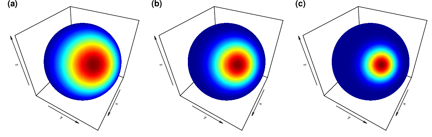
where $A_{p-1}=2\pi^{p/2}/\Gamma(p/2)$ is the hypervolume or surface area of $\mathbb{S}^{p-1}$ and $\Gamma(\cdot)$ is the standard Gamma function. Roughly speaking, the concentration parameter $\lambda$ is an inverse of variance in an epistemological sense as shown in Figure 3 where a large $\lambda$ leads to concentrated mass at the vicinity of $\mu$ and a small $\lambda$ shows dispersed distribution of the mass over a larger support.

It was observed from Equation (6) that maximum likelihood estimation of $\mu$ is equivalent to the Fréchet mean problem that minimizes sum of squared distances. We illustrate a more general case of weighted Fréchet mean problem for future use in fitting a mixture model. Given a random sample $\mathbf{X}=\{x_{1},\ldots,x_{n}\}$ and non-negative weights $\mathbf{w}=\{w_{1},\ldots,w_{n}\}$, the weighted Fréchet mean problem is given by

hence the maximum likelihood estimate $\hat{\mu}_{\text{MLE}}$ is a solution to the special case of Equation (9) when all weights $w_{i}$’s are set equal such as $w_{i}=1/n$ from an empirical measure point of view.

The hands-on choice in optimization on manifolds is Riemannian gradient descent (Absil et al. 2008). The gradient descent algorithm for a function $f(x):\mathbb{R}^{d}\rightarrow\mathbb{R}$ evolves iterates along a path characterized by local gradient evaluations, i.e., $x^{(t+1)}=x^{(t)}-\alpha\nabla f(x^{(t)})$ for some step-size $\alpha$. For a scalar-valued function on a Riemannian manifold $\mathcal{M}$, the gradient is formerly defined as a vector field. This means for each point $p\in\mathcal{M}$, $\text{grad}f\rvert_{p}$ is a tangent vector in $T_{p}\mathcal{M}$ so that the resulting update rule requires an additional step to push at iterate tangent vector onto $\mathcal{M}$ using an exponential map. Since $\text{grad}~d^{2}(x,y)=-2\textrm{Log}_{x}y$ for $x,y\in\mathcal{M}$ which can be easily shown using the variation of energy, we can write the gradient of Equation (9) at iteration $t$ as

and the final updating rule is given by

for an initial point $\mu^{(0)}$ and step-size $\alpha^{(t)}$. Explicit forms for exponential and logarithmic maps are given in Equations (2) and the procedure for location estimation is summarized in Algorithm 1.

We illustrate components of the Algorithm 1. First, we use an initial starting point $\mu^{(0)}=\sum_{i=1}^{n}w_{i}x_{i}/\|\sum_{i=1}^{n}w_{i}x_{i}\|$. When $w_{i}$’s are all equal, this corresponds to an extrinsic mean (Bhattacharya and Bhattacharya 2012) or an estimate for a location parameter of the vMF distribution. When the support condition of Theorem 3.1 is satisfied, estimates of both extrinsic and intrinsic means are contained in a convex geodesic ball. In addition to computational benefit that obtaining an extrinsic mean involves addition of vectors and $L_{2}$ normalization, it is a reasonable choice of starting point to have a small number of iterations for convergence. Second, the step-size parameter $\alpha^{(t)}$ can be determined by line search or simply set as a fixed scalar. The latter strategy was used in Algorithm 1 of Hauberg 2018 with $\alpha=0.25$. This approach has trade-offs in the sense that a fixed step-size may incur additional iterations while it avoids repetitive evaluations of the objective function during a single line search. Finally, the stopping criterion $\|\nabla f|_{\mu^{(t)}}\|<\epsilon$ is motivated from the fact that $d^{2}(x,y)=\|\text{Log}_{x}y\|^{2}$ for $x,y\in\mathbb{S}^{p}$ with the canonical metric. Also $\|\mu^{(t)}-\mu^{(t+1)}\|$ is justified from the fact that for a Riemannian manifold $\mathcal{M}$ embedded in Euclidean space, intrinsic and extrinsic distances converge as two points get sufficiently close, i.e., $\lim_{x\rightarrow y}d(x,y)/\|x-y\|=1$.

The maximum likelihood estimation for concentration parameter $\lambda$ is equivalent to solve the following optimization problem

Theorem 3.1 showed that the problem (7) has a unique critical point so that the optimization with respect to $\lambda$ can be cast as a root-finding problem of $g^{\prime}(\lambda)=0$.

Householder’s method is a class of univariate root-finding algorithms when the target function is $d$ times continuously differentiable (Householder 1970). For solving $f(x)=0$ where the function has continuous derivatives up to order $d$, the method iterates by

starting from an initial point $x^{(0)}$. For low orders $d=1$ and $2$, the updating rule in Equation (10) translates to those found from the Newton’s and Halley’s method, respectively. Therefore, we derive the updating rules to solve $g^{\prime}(\lambda)=0$ using Householder’s methods of orders 1 and 2 as follows,

beginning with an initial guess $\lambda^{(0)}\in\mathbb{R}^{+}$.

Both updating rules involve evaluation of derivatives up to order 2 or 3 at each iteration, which may incur numerical instabilities due to computational reasons such as integrating high-order terms and others. In order to make computation more robust, we employ the centered finite difference schemes using the five-point utensil

for a sufficiently small step-size $h>0$ and the derivatives are approximated by a term of order $h^{2}$ (Burden et al. 2016). By plugging in the approximate derivatives (12) to the updating rules in Equations (11), we get

where $A^{(t)}=g(\lambda^{(t)}+h)-g(\lambda^{(t)}-h)$ and others defined similarly.

We close this section by noting that computational complexities of the exact and approximate methods are compatible. At each iteration, the approximate Newton’s method shown in Equation (13) requires 3 integral evaluations, which is same as that of the exact Newton’s method (11a). While the exact Halley’s method (11b) evaluates $Z_{p}^{(k)}(\lambda)$ for $k=0,\ldots,3$, the approximate Halley’s algorithm requires an additional integral computation to evaluates five points around $\lambda^{(t)}$. However, the added computational cost is very thin since the integrand well behaves and the domain of integration is small.

We first compare performances of several algorithms that were proposed for the maximum likelihood estimation of location and concentration parameters. Given two fixed parameters $\mu_{0}=(0,0,0,0,0,1)$ and $\lambda_{0}=10$ for the SN distribution on the 5-dimensional sphere $\mathbb{S}^{5}$, we assess how performance measures such as accuracy and wall-clock time for each run of an algorithm change as the number of observations $n$ varies from 25 to 475. We repeat each run 100 times and report empirical distributions of the performance measures. We used the stopping criterion $\epsilon=10^{-8}$, which approximately equals to a square root of machine epsilon in double precision.

First, we compare two step-size rules, line search and fixed size $\alpha=0.25$, for the location parameter estimation problem. Let $\hat{\mu}_{\text{MLE}}=\hat{\mu}_{\text{MLE}}(\mathbf{X}_{1:n})$ be a maximum likelihood estimate for a random sample of size $n$. The accuracy is represented by an error quantity $\|\hat{\mu}_{\text{MLE}}-\mu_{0}\|$. For varying $n$, the results are shown in Figure 5 that as $n$ gets larger, we obtain better estimates via either of the step-size rules while the computation cost increases as expected. One notable observation is that two rules are almost parallel in both estimation quality and computational cost. The latter phenomenon seems especially interesting. It is obvious that a single update with line search should outperform that with a fixed step-size rule. However, the line search requires repetitive evaluation of the cost function in a single iterate in that its accurate update compromises overall efficiency, leading to comparable computational costs in the end.

We used the same approach for approximate Newton’s and Halley’s methods, which are compared along with two derivative-free optimization algorithms. One is optimize, a default optimization routine in R (R Core Team 2021) which combines golden section search and successive parabolic interpolation (Brent 2002). We will denote the routine as Roptim. Next, DE stands for the celebrated differential evolution algorithm that approximates the global optimum for a real-valued function using a heuristic approach (Storn and Price 1997; Mullen et al. 2011). Accuracy of an estimate $\hat{\lambda}_{\text{MLE}}=\hat{\lambda}_{\text{MLE}}(\mathbf{X}_{1:n})$ is measured by relative error $|\hat{\lambda}_{\text{MLE}}-\lambda_{0}|/\lambda_{0}$ and the same level of stopping criterion $\epsilon=10^{-8}$ is used for all testings. Performance measures are shown in Figure 5 where both approximate Newton’s and Halley’s methods consistently outperform the other two with smaller errors and shorter wall-clock time.

We also perform extensive simulations for performance comparison of the estimation algorithms with varying number of observations $n=50,100,150,200$. Table 7 summarizes performance measures in the location estimation problem for dimensions $p=5,10,20$ and concentrations $\lambda=5,10,50$. In every setting, we observed that line search and fixed step-size update rules perform almost tantamountly. Results from the concentration estimation problem are given by Table 8 for $p=5,10,20$ and $\lambda=1,5,10,20$, which show the same pattern as a fixed setting case that Newton’s and Halley’s methods show similar results while both have superior performance to the other two algorithms.

We consider two simulated examples, small-mix and large-mix, to validate clustering performance of the finite mixture of SN distributions, which are taken from Banerjee et al. 2005 and slightly modified.

First, the small-mix example draws a random sample from a mixture of two SN components with parameters $(\mu_{1},\lambda_{1})=([-0.251,-0.968],10)$ and $(\mu_{2},\lambda_{2})=([0.399,0.917],2)$ on $\mathbb{S}^{1}\subset\mathbb{R}^{2}$. For each component, 100 observations are randomly drawn.

A random sample and some clustering results are given in Figure 6 Both spkmeans and vMF-soft showed a slight misclassification for the bottom-most observations of the 2nd class in contrast to SN-soft. The same test was repeated 10 times and average clustering quality indices are reported in Table 2 with different numbers of clusters $K=2,3$ and $4$. When $K=2$, both SN and vMF mixtures performed well while the former had slightly better results. When $K>2$, SN mixtures had less accurate results than vMF mixtures, which is reasonable and rather convincing to claim fitness of SN mixtures since the true model consists of SN components and inflated quality indices of vMF mixtures may potentially confuse the decision given such results. It is not surprising that spkmeans showed compatible result as a limit of vMF mixture model. In the small-mix example, the data has two linearly separable components so that the $k$-means algorithm performed competitively.

The large-mix example considers a mixture density on $\mathbb{S}^{3}$ that is composed of 3 SN distributions with location parameters that are drawn randomly to reside in different quadrants, concentration parameters $(\lambda_{1},\lambda_{2},\lambda_{3})=(40,20,60)$. Component weights are chosen as follows. Draw $u_{i}\sim U(9,11)$ for $i=1,2,3$ and set $\pi_{i}=u_{i}/\sum_{i=1}^{3}u_{i}$, which assigns almost equal weights for individual components. We draw a random sample of 3000 observations according to the specified mixture model and the results for average of 10 runs are reported in Table 3.

Since we are using large concentration parameters with mutually distant locations, it is expected that observations per class should have little overlapping support and any good model should be able to detect three distinct clusters. In other words, a quality index should be low for $K=2,4$ and high for $K=3$. Except for the $k$-means, all algorithms perform exceptionally well when $K=3$. However, the desired pattern is only observed for SN mixtures and spkmeans though the latter sometimes does not decrease as much as the former. It is worth to mention that vMF mixtures even show higher quality indices when $K=4$.

We now validate clustering performance of the proposed mixture model with SN distributions on two real data - household and Classic3.

The household data is part of a survey data of household expenditures on commodity groups such as housing, goods, service, and food among 20 single males and females (Hothorn and Everitt 2014). We follow the convention of Hornik and Grün 2014 to focus on relative portion of total expenditures for housing, service, and food categories only. Each individual’s expenditure profile in $\mathbb{R}^{3}$ is projected onto $\mathbb{S}^{2}$ by $L_{2}$ normalization $x\leftarrow x/\|x\|$. As a preliminary step, we fitted the SN distribution to expenditures of males and females separately whose maximum likelihood estimates are shown in Table 4. We note that the females’ expenditures have a larger concentration by $\hat{\lambda}_{\text{MLE}}=95.743$ while the males show much dispersed pattern as indicated by $\hat{\lambda}_{\text{MLE}}=19.638$.

References

- (1)
- Absil et al. (2008) Absil, P.-A., Mahony, R. and Sepulchre, R. (2008). Optimization Algorithms on Matrix Manifolds, Princeton University Press, Princeton, N.J. ; Woodstock.
- Afsari (2011) Afsari, B. (2011). RIEMANNIAN Lp CENTER OF MASS: EXISTENCE, UNIQUENESS, AND CONVEXITY, Proceedings of the American Mathematical Society 139(2): 655–673.
- Aggarwal et al. (2004) Aggarwal, G., Chowdhury, A. K. R. and Chellappa, R. (2004). A system identification approach for video-based face recognition, Proceedings of the Pattern Recognition, 17th International Conference on (ICPR’04) Volume 4 - Volume 04, ICPR ’04, IEEE Computer Society, USA, pp. 175–178.
- Akaike (1974) Akaike, H. (1974). A new look at the statistical model identification, IEEE Transactions on Automatic Control 19(6): 716–723.
- Arnaudon et al. (2013) Arnaudon, M., Barbaresco, F. and Yang, L. (2013). Medians and Means in Riemannian Geometry: Existence, Uniqueness and Computation, in F. Nielsen and R. Bhatia (eds), Matrix Information Geometry, Springer Berlin Heidelberg, Berlin, Heidelberg, pp. 169–197.
- Banerjee et al. (2005) Banerjee, A., Dhillon, I. S., Ghosh, J. and Sra, S. (2005). Clustering on the unit hypersphere using von mises-fisher distributions, Journal of Machine Learning Research 6(46): 1345–1382.
- Bhattacharya and Bhattacharya (2012) Bhattacharya, A. and Bhattacharya, R. N. (2012). Nonparametric Inference on Manifolds: With Applications to Shape Spaces, number 2 in Institute of Mathematical Statistics Monographs, Cambridge University Press, Cambridge, UK ; New York.
- Bhattacharya and Dunson (2012) Bhattacharya, A. and Dunson, D. (2012). Nonparametric Bayes classification and hypothesis testing on manifolds, Journal of Multivariate Analysis 111: 1–19.
- Bishop (2006) Bishop, C. M. (2006). Pattern Recognition and Machine Learning, Information Science and Statistics, Springer, New York.
- Bissacco et al. (2001) Bissacco, A., Chiuso, A., Yi Ma and Soatto, S. (2001). Recognition of human gaits, Proceedings of the 2001 IEEE Computer Society Conference on Computer Vision and Pattern Recognition. CVPR 2001, Vol. 2, IEEE Comput. Soc, Kauai, HI, USA, pp. II–52–II–57.
- Bouveyron et al. (2019) Bouveyron, C., Celeux, G., Murphy, T. B. and Raftery, A. E. (2019). Model-Based Clustering and Classification for Data Science: With Applications in R, first edn, Cambridge University Press.
- Brent (2002) Brent, R. P. (2002). Algorithms for Minimization without Derivatives, Dover Publications, Mineola, N.Y.
- Burden et al. (2016) Burden, R. L., Faires, J. D. and Burden, A. M. (2016). Numerical Analysis, tenth edition edn, Cengage Learning, Boston, MA.
- Cavanaugh (1997) Cavanaugh, J. E. (1997). Unifying the derivations for the Akaike and corrected Akaike information criteria, Statistics & Probability Letters 33(2): 201–208.
- Dempster et al. (1977) Dempster, A. P., Laird, N. M. and Rubin, D. B. (1977). Maximum Likelihood from Incomplete Data Via the EM Algorithm, Journal of the Royal Statistical Society: Series B (Methodological) 39(1): 1–22.
- Dhillon et al. (2003) Dhillon, I. S., Mallela, S. and Modha, D. S. (2003). Information-theoretic co-clustering, Proceedings of the Ninth ACM SIGKDD International Conference on Knowledge Discovery and Data Mining, KDD ’03, Association for Computing Machinery, New York, NY, USA, pp. 89–98.
- Dhillon and Modha (2001) Dhillon, I. S. and Modha, D. S. (2001). Concept Decompositions for Large Sparse Text Data Using Clustering, Machine Learning 42(1/2): 143–175.
- do Carmo (1992) do Carmo, M. P. (1992). Riemannian Geometry, Mathematics. Theory & Applications, Birkhäuser, Boston.
- Fisher (1953) Fisher, R. (1953). Dispersion on a Sphere, Proceedings of the Royal Society A: Mathematical, Physical and Engineering Sciences 217(1130): 295–305.
- Fletcher et al. (2009) Fletcher, P. T., Venkatasubramanian, S. and Joshi, S. (2009). The geometric median on Riemannian manifolds with application to robust atlas estimation, NeuroImage 45(1): S143–S152.
- Fréchet (1948) Fréchet, M. R. (1948). Les éléments aléatoires de nature quelconque dans un espace distancié, Annales de l’institut Henri Poincaré 10(4): 215–310.
- Goodall and Mardia (1999) Goodall, C. R. and Mardia, K. V. (1999). Projective shape analysis, Journal of Computational and Graphical Statistics 8(2): 143–168.
- Gopal and Yang (2014) Gopal, S. and Yang, Y. (2014). Von mises-fisher clustering models, in E. P. Xing and T. Jebara (eds), Proceedings of the 31st International Conference on Machine Learning, Vol. 32 of Proceedings of Machine Learning Research, PMLR, Bejing, China, pp. 154–162.
- Grove and Karcher (1973) Grove, K. and Karcher, H. (1973). How to conjugate C1-close group actions, Mathematische Zeitschrift 132(1): 11–20.
- Hannan and Quinn (1979) Hannan, E. J. and Quinn, B. G. (1979). The determination of the order of an autoregression, Journal of the Royal Statistical Society. Series B (Methodological) 41(2): 190–195.
- Hastie et al. (2009) Hastie, T., Tibshirani, R. and Friedman, J. H. (2009). The Elements of Statistical Learning: Data Mining, Inference, and Prediction, Springer Series in Statistics, 2nd ed edn, Springer, New York, NY.
- Hauberg (2018) Hauberg, S. (2018). Directional Statistics with the Spherical Normal Distribution, 2018 21st International Conference on Information Fusion (FUSION), IEEE, Cambridge, United Kingdom, pp. 704–711.
- Hornik and Grün (2014) Hornik, K. and Grün, B. (2014). movMF : An R Package for Fitting Mixtures of von Mises-Fisher Distributions, Journal of Statistical Software 58(10).
- Hothorn and Everitt (2014) Hothorn, T. and Everitt, B. (2014). A Handbook of Statistical Analyses Using R, third edition edn, CRC Press, Taylor & Francis Group, Boca Raton.
- Householder (1970) Householder, A. S. (1970). The Numerical Treatment of a Single Nonlinear Equation, McGraw-Hill, London.
- Jaccard (1912) Jaccard, P. (1912). THE DISTRIBUTION OF THE FLORA IN THE ALPINE ZONE.1, New Phytologist 11(2): 37–50.
- Jupp and Mardia (1979) Jupp, P. E. and Mardia, K. V. (1979). Maximum Likelihood Estimators for the Matrix Von Mises-Fisher and Bingham Distributions, The Annals of Statistics 7(3).
- Kendall (1990) Kendall, W. S. (1990). Probability, Convexity, and Harmonic Maps with Small Image I: Uniqueness and Fine Existence, Proceedings of the London Mathematical Society s3-61(2): 371–406.
- Lee (1997) Lee, J. M. (1997). Riemannian Manifolds: An Introduction to Curvature, number 176 in Graduate Texts in Mathematics, Springer, New York.
- Ley and Verdebout (2017) Ley, C. and Verdebout, T. (2017). Modern Directional Statistics, Chapmann & Hall/CRC Interdisciplinary Statistics Series, CRC Press, Taylor & Francis Group, Boca Raton London New York.
- Macqueen (1967) Macqueen, J. (1967). Some methods for classification and analysis of multivariate observations, In 5-Th Berkeley Symposium on Mathematical Statistics and Probability, pp. 281–297.
- Mardia and Jupp (2000) Mardia, K. V. and Jupp, P. E. (2000). Directional Statistics, Wiley Series in Probability and Statistics, J. Wiley, Chichester ; New York.
- McLachlan et al. (2019) McLachlan, G. J., Lee, S. X. and Rathnayake, S. I. (2019). Finite Mixture Models, Annual Review of Statistics and Its Application 6(1): 355–378.
- Mullen et al. (2011) Mullen, K., Ardia, D., Gil, D., Windover, D. and Cline, J. (2011). DEoptim: An R package for global optimization by Differential Evolution, Journal of Statistical Software 40(6): 1–26.
- Patrangenaru and Ellingson (2016) Patrangenaru, V. and Ellingson, L. (2016). Nonparametric Statistics on Manifolds and Their Applications to Object Data Analysis, CRC Press, Taylor & Francis Group, Boca Raton.
- Pennec (2006) Pennec, X. (2006). Intrinsic Statistics on Riemannian Manifolds: Basic Tools for Geometric Measurements, Journal of Mathematical Imaging and Vision 25(1): 127–154.
- Pennec et al. (2020) Pennec, X., Sommer, S. and Fletcher, T. (2020). Riemannian Geometric Statistics in Medical Image Analysis, Academic Press, San Diego.
- R Core Team (2021) R Core Team (2021). R: A Language and Environment for Statistical Computing, R Foundation for Statistical Computing, Vienna, Austria.
- Rand (1971) Rand, W. M. (1971). Objective Criteria for the Evaluation of Clustering Methods, Journal of the American Statistical Association 66(336): 846–850.
- Schwarz (1978) Schwarz, G. (1978). Estimating the Dimension of a Model, The Annals of Statistics 6(2).
- Sra (2012) Sra, S. (2012). A short note on parameter approximation for von Mises-Fisher distributions: And a fast implementation of I s (x), Computational Statistics 27(1): 177–190.
- Storn and Price (1997) Storn, R. and Price, K. (1997). Differential Evolution – A Simple and Efficient Heuristic for global Optimization over Continuous Spaces, Journal of Global Optimization 11(4): 341–359.
- Strehl and Ghosh (2002) Strehl, A. and Ghosh, J. (2002). Cluster Ensembles — a Knowledge Reuse Framework for Combining Multiple Partitions, Journal of Machine Learning Research 3: 583–617.
- You and Park (2021) You, K. and Park, H.-J. (2021). Re-visiting Riemannian geometry of symmetric positive definite matrices for the analysis of functional connectivity, NeuroImage 225: 117464.